Letter

Interweaving the Principle of Least Potential Energy in School and Introductory University Physics Courses

1
Department of Physics and Project Unit, Sapir Academic College, Sderot, Hof Ashkelon 79165, Israel
2
Department of Science and Technology Education, Ben-Gurion University of Negev, P.O.B. 653, Beer-Sheva 8410501, Israel
3
Department of Solar Energy and Environmental Physics, Jacob Blaustein Institute for Desert Research, Ben-Gurion University of Negev, P.O.B. 653, Beer-Sheva 8410501, Israel
*
Author to whom correspondence should be addressed.
Symmetry 2017, 9(3), 45; https://doi.org/10.3390/sym9030045
Submission received: 15 December 2016 / Revised: 16 March 2017 / Accepted: 16 March 2017 / Published: 22 March 2017

Abstract

:
Understanding advanced physical phenomena such as vertically hanging elastic column, soap bubbles, crystals and cracks demands expressing and manipulating a system’s potential energy under equilibrium conditions. However, students at schools and universities are usually required to consider the forces acting on a system under equilibrium conditions, rather than taking into account its potential energy. As a result, they find it difficult to express the system’s potential energy and use it for calculations when they do need to do so. The principle of least potential energy is a powerful idea for solving static equilibrium physics problems in various fields such as hydrostatics, mechanics, and electrostatics. In the current essay, the authors describe this principle and provide examples where students can apply it. For each problem, the authors provide both the force consideration solution approach and the energy consideration solution approach.

1. Introduction

Analyzing physics problems often requires one to understand how to apply conditions for static equilibrium in those problems. Usually, in school physics courses as well as in introductory physics courses students mainly learn that there are two conditions one has to impose in such problems: (a) zero resultant force; and (b) zero resultant torque about any axis.
Imposing these two conditions is the usual problem solving strategy in these courses. However, more advanced topics, such as rotating and self-gravitating liquid masses of homogenous liquids (cf. [1], or higher level mechanics problems requires one to consider the system’s overall energy, instead of the net force and torque. Additionally, sometimes it is more beneficial to break the system into several subsets of problems. In these cases, applying a “greedy algorithm” approach in which finding the local energetic minima of the subset, sometimes yields the overall energetic minima of the system. Students who are not used to consider the energetic view present difficulties in understanding quantum mechanical descriptions such as a particle in a box or the energy levels of electrons in an atom.
We therefore suggest exposing students to energetic conditions and calculations already in high school and introductory courses at colleges and universities. In addition, students’ school experiences with the concept of energy leads many to view energy as traveling through machines and wires and changing appearances at different points—what Duit (1987) calls a quasi-material conception [2]. We believe that this view is caused because students are used to applying the concept of energy in dynamic situations. Applying the least potential energy principle under equilibrium situations may assist students to acquire better understanding of the energy concept as an abstract idea rather than a traveling material. In this paper, we first introduce the principle of least potential energy and second, offer three examples taken from the fields of hydrostatics, electricity, and mechanics to demonstrate how to apply the least of potential energy principle.

2. Description of the Principle of Least Potential Energy

The least potential energy principle states that a physical system subjected to potential forces i.e., forces that are given by a gradient of conservative field will take the lowest potential energy. In other words, according to this principle, and under those conditions, a system of bodies at rest will have adopted a configuration that minimizes the total potential energy (a phenomenon called by Euler “effort”). This means that in equilibrium the gradient of the total system’s potential energy equals to zero. Mathematically, we may write this as:
U x = U y = U z = 0
where U is the potential energy, and is a smooth function by definition.
Equation (1) can be obtained from the zero-resultant force condition in equilibrium ( F = 0 ). It is known that when conservative forces are involved we may write:
F = g r a d U
Since the total force, F, in equilibrium equals zero, we get Equation (1).
Mathematically, applying Equation (1) on a physic’s problem rather than trying to solve the zero-resultant force equation might be easier. In this way, the problem reduces to finding stationary points by taking derivatives of a scalar function and solving scalar equations, with no need of vector algebra. For systems with more than one degree of freedom this task becomes more difficult but one can still find numerical solutions. More general and sophisticated methods of solving static problems include Lagrange multipliers and the calculus of variations [3].
The principle of least potential energy is actually a private case or a static version of the least action principle. According to the least action principle, the motion of a physical system from time t 1 to time t 2 is such that the following line integral,
S = t 1 t 2 ( T U ) d t
where T is the kinetic energy, an extremum relative to all other paths. It was shown that the path with the minimal action is the one satisfying Newton’s second law [4]. It is clear that for stationary system the principle of least action is reduced to the principle of least potential energy since T = 0 and the potential energy U is time independent. The least action principle, which is one of the greatest generalizations in all physical science, was first formulated by Maupertuis in 1746 [5]. This metaphysical idea was further mathematically developed by the works of Euler, Lagrange, Jacobi and finally formulated by Hamilton and known as Hamilton’s principle [6].

3. Examples Demonstrating the Use of the Least Potential Energy Principle

The following three examples will be demonstrated: (a) fluid static in a piston of small cross-sectional area; (b) a system of point charges; and (c) the catenary problem. Each problem will be first solved by applying the zero-resultant force condition to the problem and than by applying the least potential energy principle.

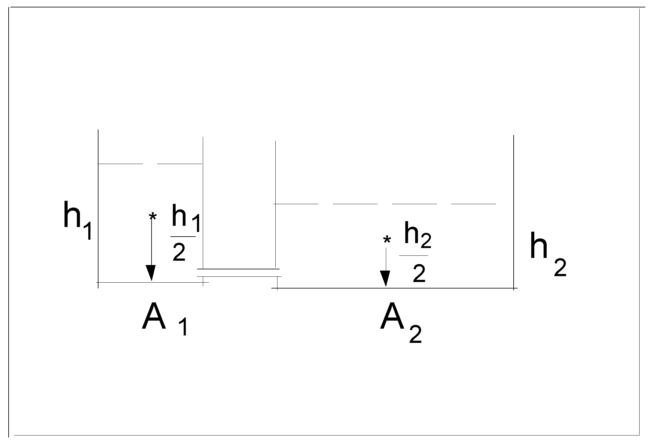
3.1. Example a: Fluid Static in a Piston of Small Cross-Sectional Area

We pour V 0 volume of water into two vessels with basis areas A 1 and A 2 , respectively. The problem is to find the heights h 1 and h 2 of the water in each vessel (see Figure 1) in the equilibrium state. The problem can be easily solved by applying the least potential energy principle. In the final state, the water is divided between the two vessels as such that their potential energy is minimal.

3.1.1. Solution Based on Newton’s Laws

It is well known [7] that for incompressible fluids the pressure inside the fluid is given by p = p 0 + ρ g h where p 0 is the atmospheric pressure on the surface of the liquid and ρ is the fluid density which is assumed to be constant. At equilibrium, the pressures at the bottom of the two vessels are equal so we write ( ρ = 1 ) that
p 0 + ρ g h 1 = p 0 + ρ g h 2
which gives h 1 = h 2 .

3.1.2. Solution Based on the Least Potential Energy Principle

Assume that the height of the water in the first vessel is h 1 and h 2 in the second where h 2 = ( V 0 h 1 A 1 ) / A 2 . The potential energy of the system is (we take the density of water as 1):
E ( h 1 , h 2 ) = h 1 A 1 h 1 2 g + h 2 A 2 h 2 2 g = g 2 ( h 1 2 A 1 + h 2 2 A 2 )
Inserting the above expression for h 2 into Equation (1) gives the total energy as a function of one variable h 1 .
E ( h 1 ) = g 2 ( h 1 2 A 1 + ( V 0 h 1 A 1 ) 2 A 2 )
To find to the stationary points, we equate the derivative of Equation (6) with respect to h 1 and solve for h 1 . Using elementary calculus, we remain with the following equation:
h 1 ( 1 + A 1 A 2 ) = V 0 A 2
which has the solution h 1 = V 0 / ( A 1 + A 2 ) . This point is indeed a minimum as Equation (6) describes an opened-up parabola. Solving for h 2 , we get h 2 = V 0 / ( A 1 + A 2 ) . We conclude that h 1 = h 2 which we already know from everyday experience, and that the pressure of liquids depends only on the height of the fluid and not on the shape of the container.
Although for this problem the Newtonian approach seems much simpler, we believe that it is very important from a pedagogic point of view to show students the “energy” solution, which emanates from the general principle of least potential energy.

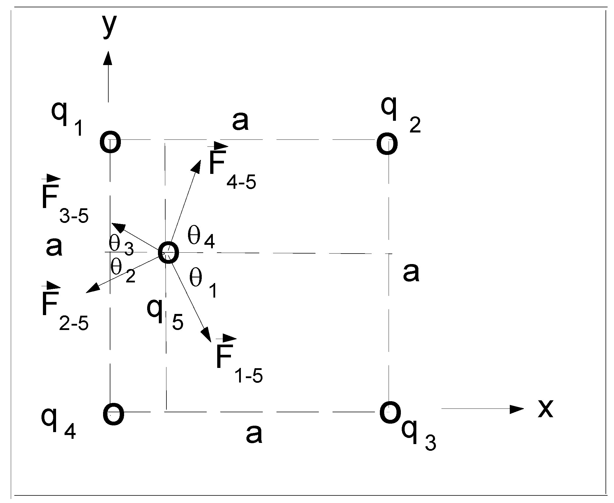
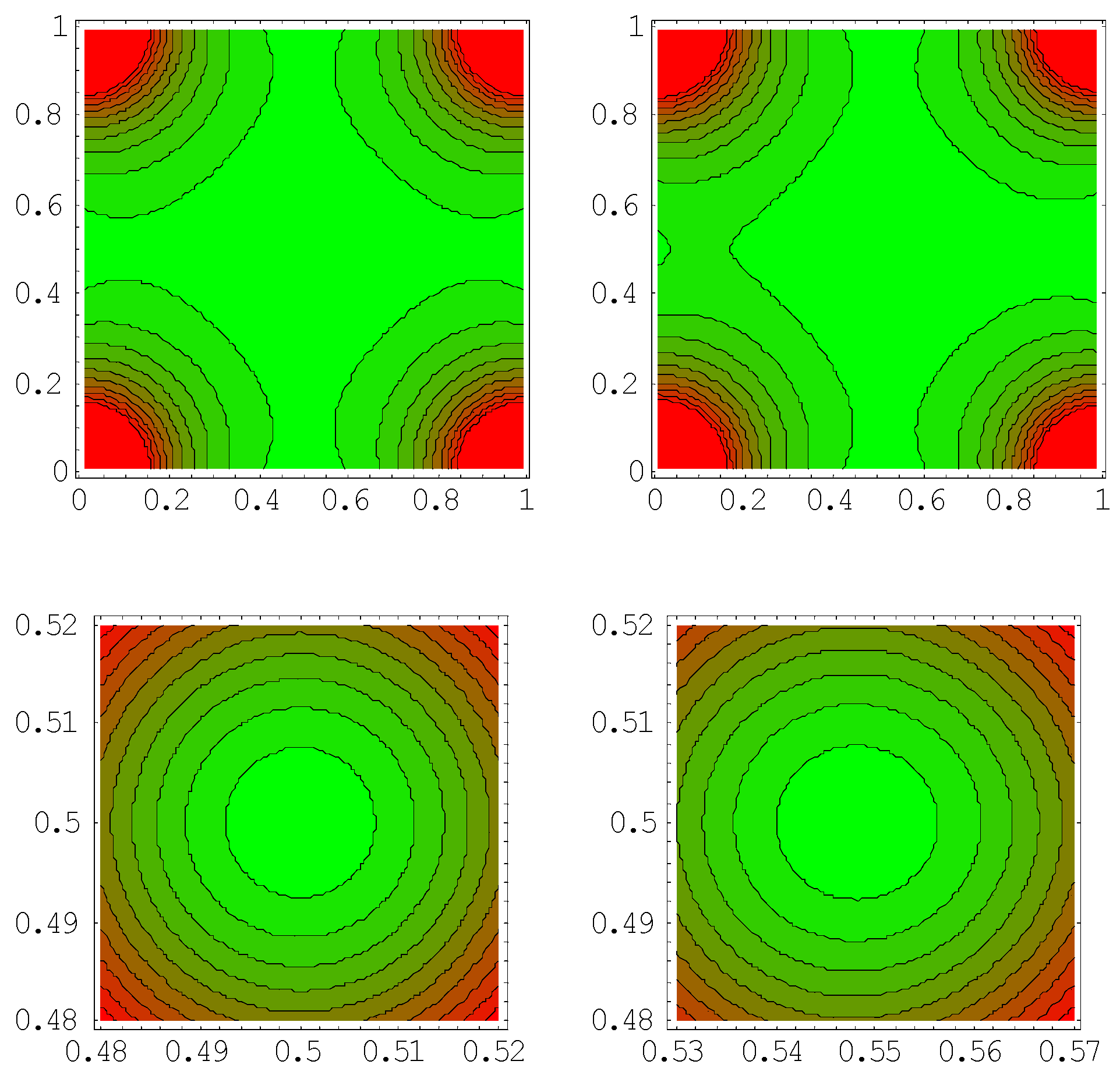
3.2. Example b: A System of Point Charges

Four positive electric charges q 1 , q 2 , q 3 and q 4 are fixed at the vertexes of a square. We have to find the place ( x , y ) of a fifth positive electric charge q 5 so it will remain in equilibrium (see Figure 2).

3.2.1. Solution Based on Newton’s Laws

Solving this problem using forces considerations is a complicated task as we have to deal with vectors quantities. In order that the q 5 will be in a static equilibrium, we demand that the resultant force F 1 5 + F 2 5 + F 3 5 + F 4 5 = 0 acting on it vanish. Writing the explicit equations in the rectangular system yields
F 1 5 cos θ 1 F 2 5 cos θ 2 F 3 5 cos θ 3 + F 4 5 cos θ 4 = 0 F 1 5 sin θ 1 F 2 5 sin θ 2 + F 3 5 sin θ 3 + F 4 5 sin θ 4 = 0
Inserting cos θ 4 = x / x 2 + y 2 and similar expressions for sin θ 4 and for the other angles into Equation (8) yield the two following coupled equations for x and y :
k ( q 1 q 5 x ( x 2 + ( a y ) 2 ) 3 / 2 q 2 q 5 ( a x ) ( ( a x ) 2 + ( a y ) 2 ) 3 / 2 q 3 q 5 ( a x ) ( ( a x ) 2 + y 2 ) 3 / 2 + q 4 q 5 x ( x 2 + y 2 ) 3 / 2 ) = 0 k ( q 1 q 5 y ( x 2 + ( a y ) 2 ) 3 / 2 q 2 q 5 ( a y ) ( ( a x ) 2 + ( a y ) 2 ) 3 / 2 + q 3 q 5 ( a y ) ( ( a x ) 2 + y 2 ) 3 / 2 + q 4 q 5 y ( x 2 + y 2 ) 3 / 2 ) = 0
where k is the electrostatic constant. Equation (9) is too complicated to solve analytically, but can be solved numerically using appropriate mathematical packages. We skip solving these equations exactly and present the energy approach for solving this problem.

3.2.2. Solution Based on the Least Potential Energy Principle

Applying the least potential energy principle overcomes this difficulty as we are left with scalar quantities. First, we write the electrostatic energy function of the system:
U ( x , y ) = U 0 + k ( q 1 q 5 x 2 + y 2 + q 2 q 5 ( a x ) 2 + y 2 + q 3 q 5 x 2 + ( a y ) 2 + q 4 q 5 ( a x ) 2 + ( a y ) 2 )
where U 0 is the electrostatic energy of the fixed four charges which is constant and does not depend on x and y . We aim to find the minimum of U ( x , y ) which is now a function of two variables. This is also not an easy analytical task. Instead, we show a contour plot of U ( x , y ) U 0 for two cases. In the first all the charges are equal to one Coulomb and in the second q 1 = 1.1 (for simplicity we choose k = 1 and a = 1 ). For the symmetric case, it is obvious that ( x , y ) = ( 0.5 , 0.5 ) is a minimum while for the asymmetric case the minimum is at ( x , y ) = ( 0.548 , 0.5 ) . We also see how the contour lines changes as we break the symmetry of the problem (Figure 3).
For the above electrostatic problem, the forces based approach is more complicated than the “energy” approach since we have to write the equations for the forces components and to solve more complicate equations. Plotting the two dimensional maps for the energy functions gives us global information about the electrostatic energy distribution from which we can get local information about the direction of the resultant force in each point. Solving these two problems show that using energy considerations and numerical solutions obtained by mathematical package improve our ability to solve complicate problems and enhance our physical understanding.

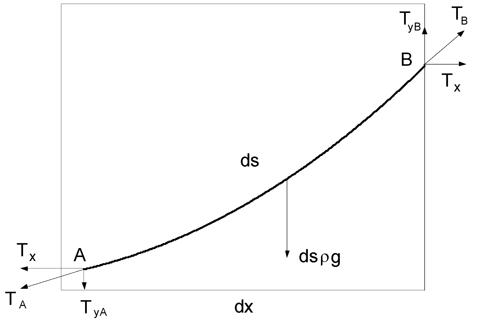
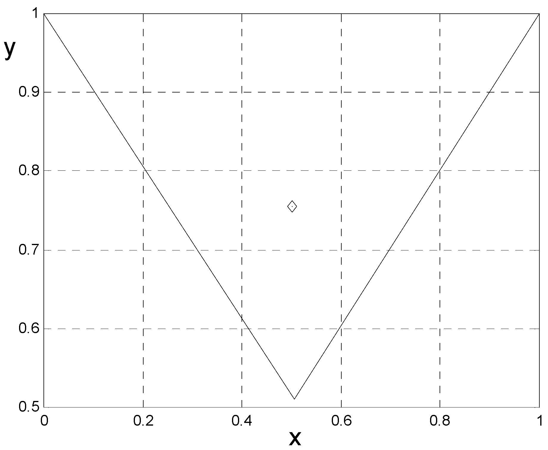
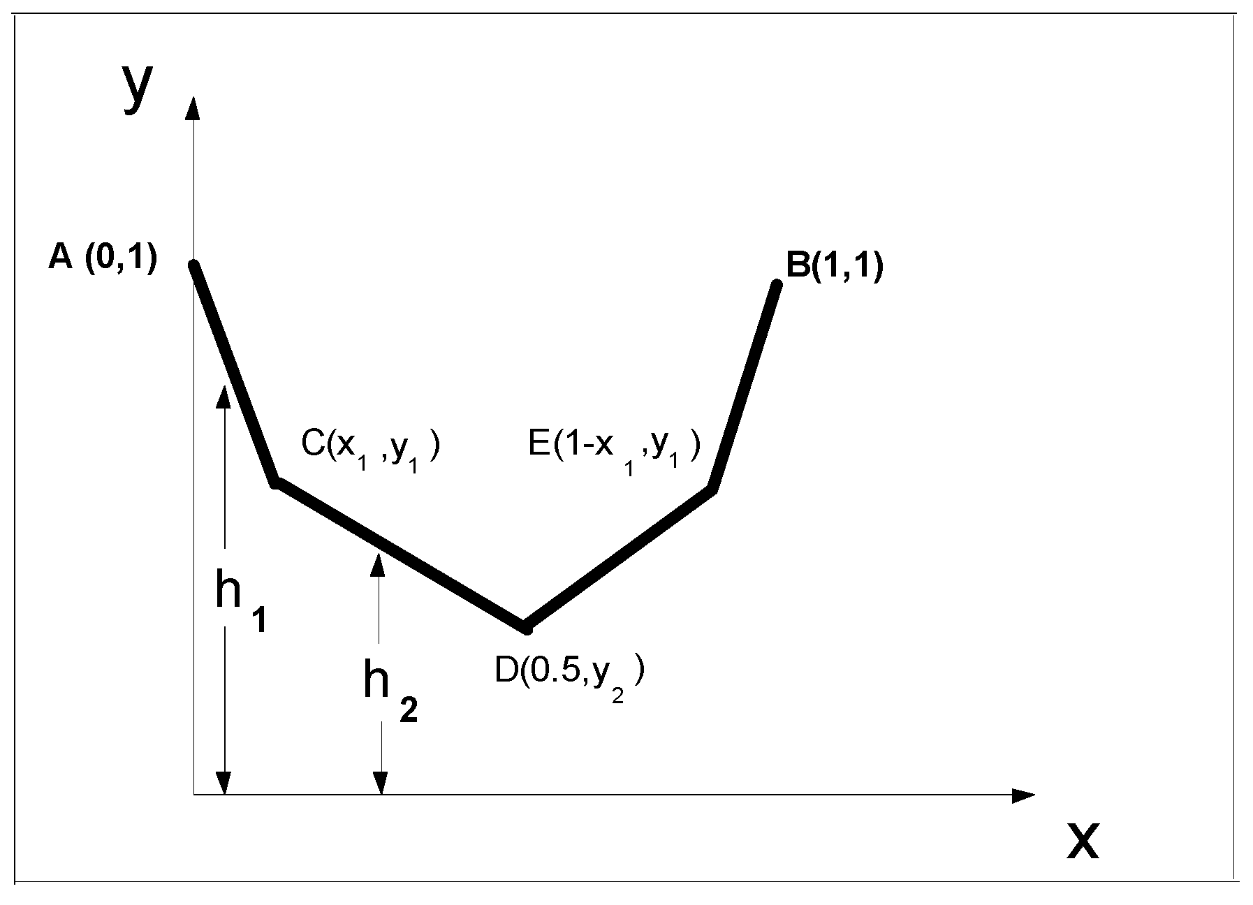
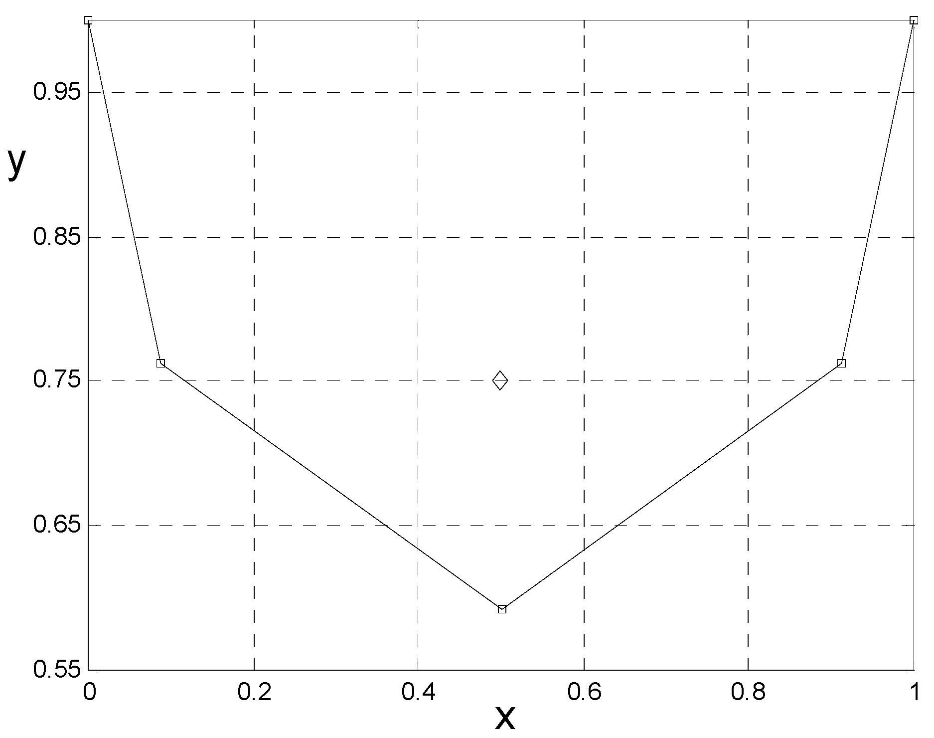
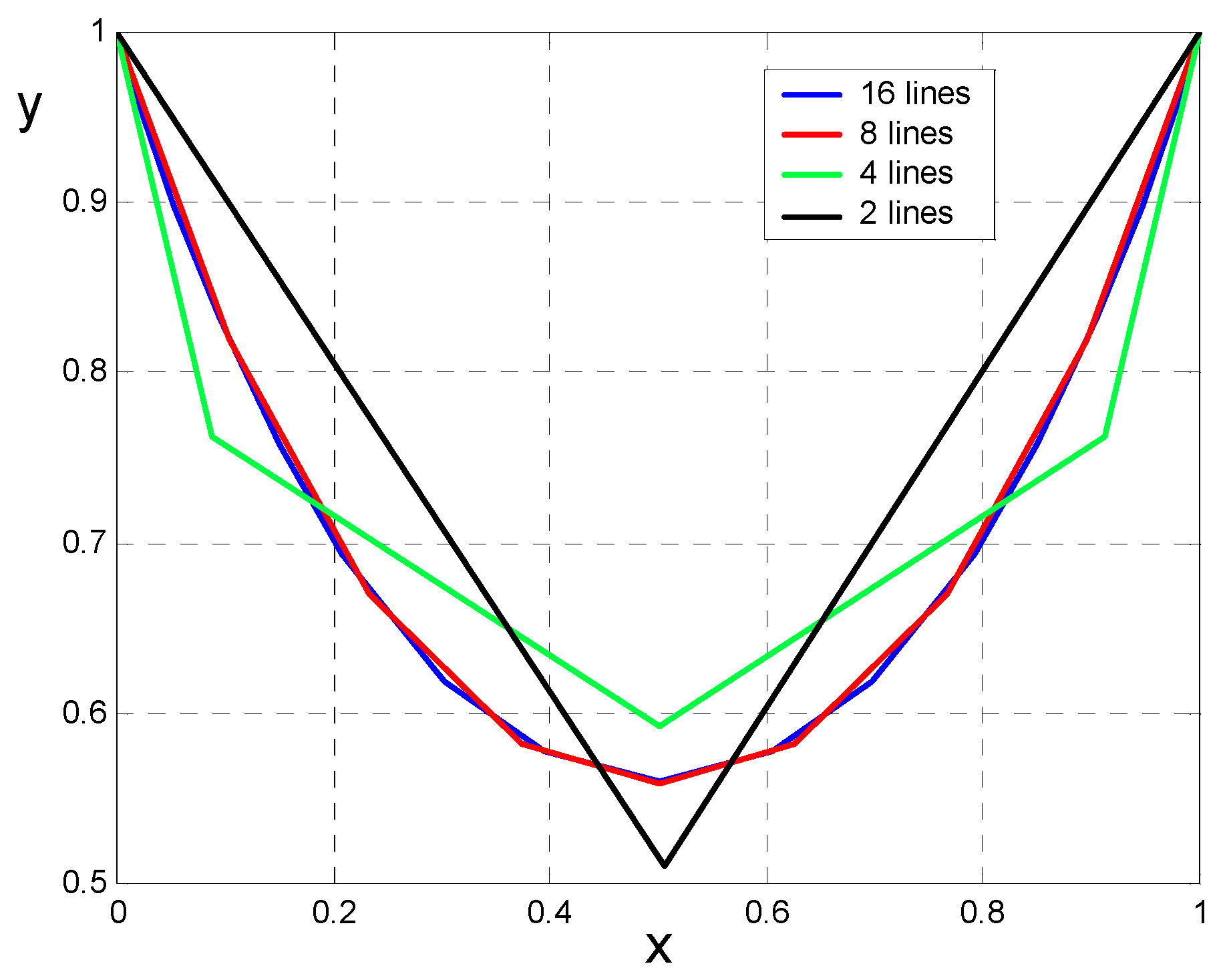
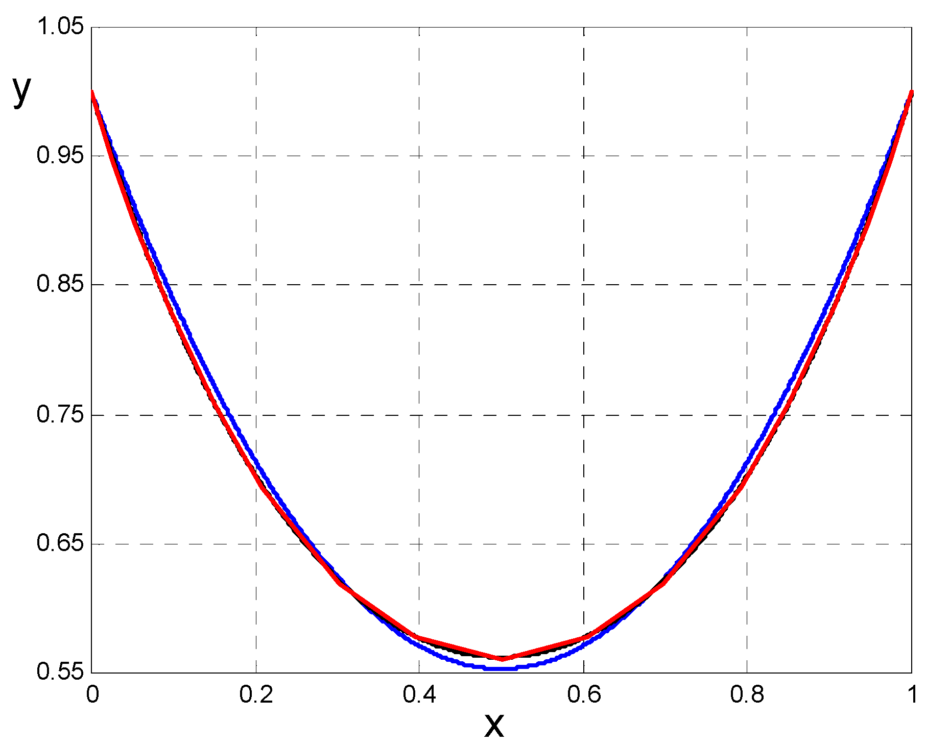
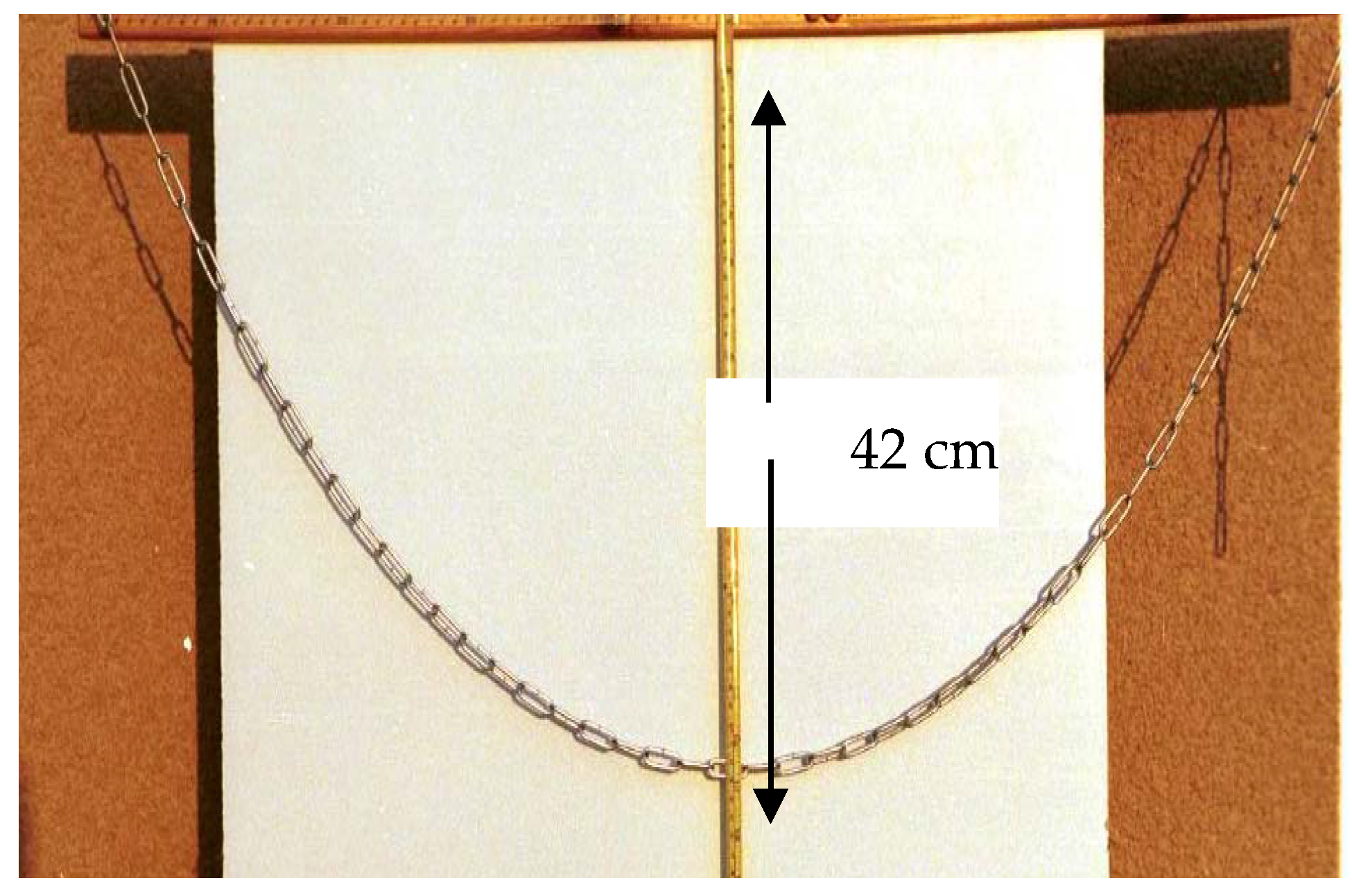
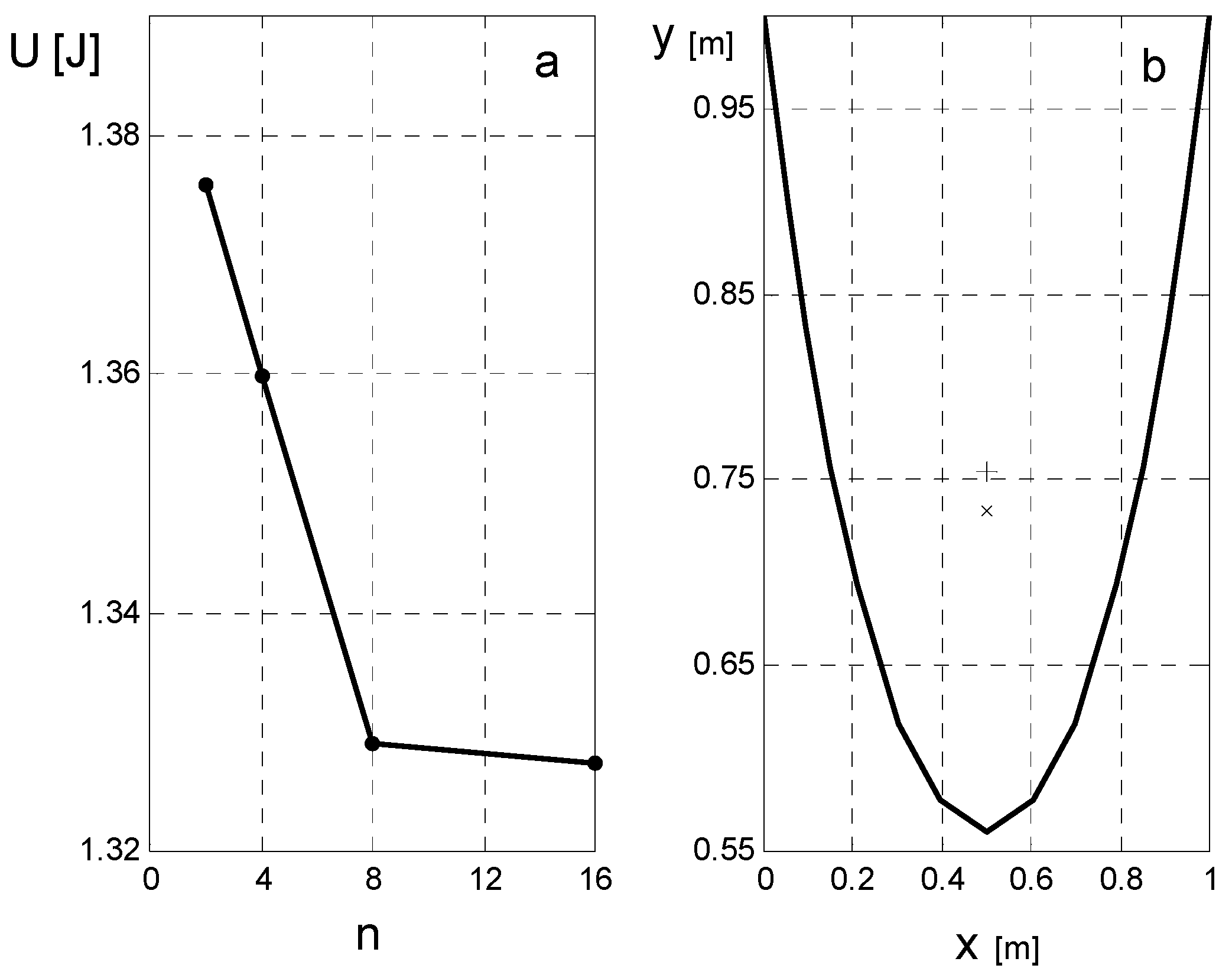
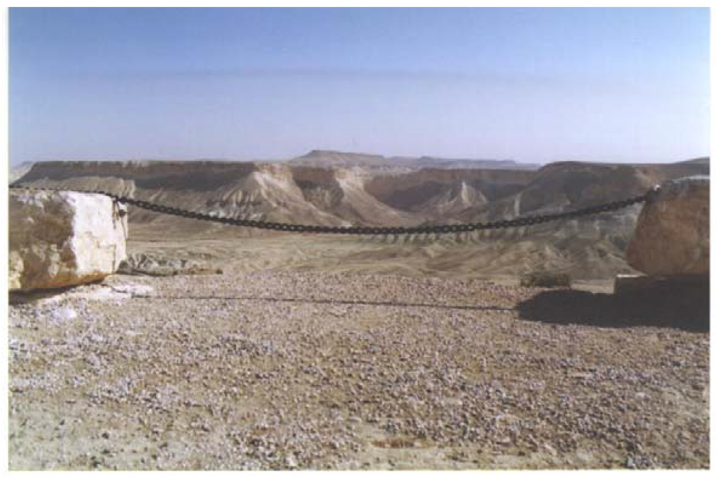
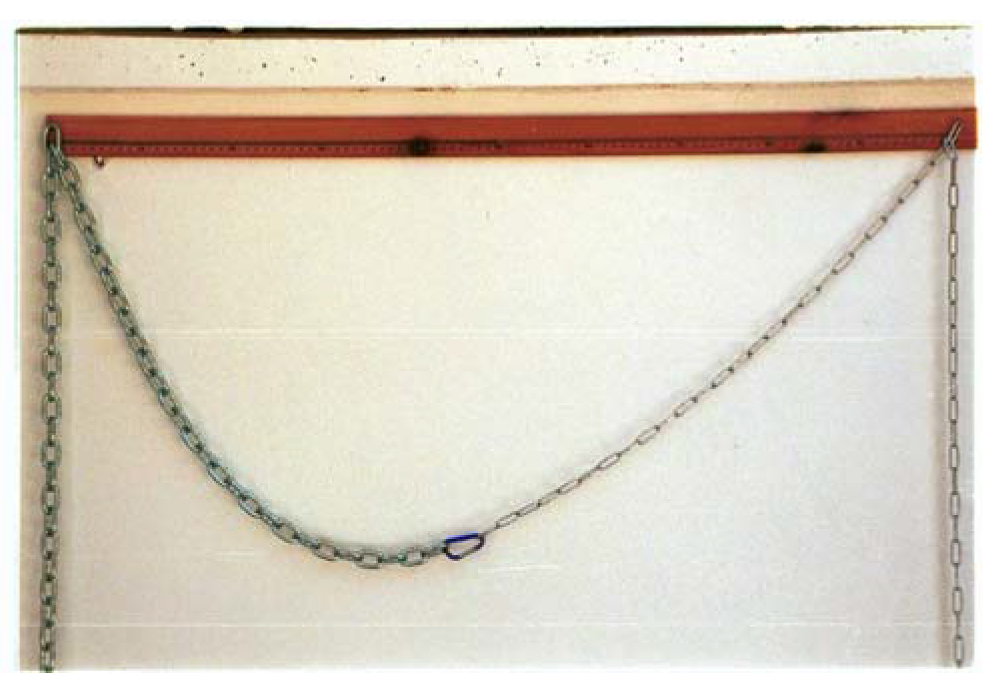
3.3. Example c: The Catenary Problem

3.3.1. Solution Based on Newton’s Laws

The problem was posed explicitly for the first time by James Bernoulli in 1690, when he asked to find the curve assumed by a flexible chain which hangs freely, fixed between two points [8,9,10,11]. Galileo was the first to investigate the catenary, which he mistook for parabola. The correct solution, which is given by hyperbolic cosine was found independently by the great mathematicians of that era, Huygens, Leibnitz and the Jhon Bernoulli the brother of James. The name catenary was first used by Huygens in a letter to Leibnitz in 1690. Any uniform cable or chain, which is subject to its own weight, describes a catenary as shown in Figure 1.
The only external force acting on the flexible chain is the gravitational force m g (we assume here that g is constant) and its shape can be obtained by applying the principle of Newtonian mechanics. First, at equilibrium, we conclude that the horizontal component of the Tension T x is equal at each point of the chain and that the vertical component of the tension is T y = T x y where y = d y / d x is the slope of the chain at a point ( x , y ) as described in Figure 4.
We proceed by considering the forces acting on a short length of chain AB subtending a horizontal distance d x and arclength d s which is equal to d s = 1 + y 2 [7]. The horizontal forces cancel each other so we consider only the vertical ones which are T y A and T y B . The sum of these tensions is equal to the weight of the chain and we obtain T y B T y B = ρ g d s where ρ is chain’s constant mass per unit length. We can use the relation T y = T x y and get
T x ( y | B y | A ) = ρ g d s
or
T x ( y | B y | A ) d x d x = ρ g d s
which gives the following second order differential equation
T x y d x = ρ g 1 + y 2 d x
Equation (11) can be integrated twice to get y ( x ) , using the boundary conditions y ( 0 ) = y ( 0 ) = 0 .
This yields the following equation for the catenary
y ( x ) = T x ρ g ( cosh ρ g x T x 1 )
T x can be further expressed in terms of the sag and the total length of the chain. To conclude, by applying Newton laws for a small segment of the chain and solving the resulting differential equation, we obtain that the catenary curve described by hyperbolic cosine and that the horizontal component of the tension is constant along the chain. This approach is “standard” in the sense that we assume that the chain obeys Newtonian laws and its shape can be found from solving the appropriate equation with specific boundary conditions [7]. The chain does not have to “know” anything else about the whole curve (Figure 5).

3.3.2. Solution Based on the Least Potential Energy Principle

In contrast to the previous approach. we assume here that in its final state the chain will be in a stable state so its overall shape will minimize its potential energy. Using the same arguments as Feynman did when he showed that Newton’s second law is equivalent to the least action principle, we can translate the grand statement about the chain to local differential statements [12]. In equilibrium, it is necessary that each small part of the chain is also in equilibrium, so it also has a minimum potential energy and the equation F i = 0 where the subscript i stands for the i th infinitesimal element of the chain holds. Thus, there is nothing mysterious in the way the chain “finds” its way towards the curve with the least potential energy. Its small element obeys Newton’s second law.
Finding the shape of hanging chain is a classic problem in the calculus of variations. Among all the infinite number of curves connecting the two end points, we have to find the one with the minimum potential energy. The complete solution of this problem is beyond the scope of high school mathematics and it is described in many textbooks of analytic mechanics [3].
To overcome this difficulty, we convert the continuous problem to a discrete version, which is simpler and more intuitive to students, as the solution is constructed step by step from a basic principle. For the two-segments catenary problem, the length constraint is
x 2 + ( y 1 ) 2 + ( 1 x ) 2 + ( 1 y ) 2 = l
and the symmetry, i.e., x = 0.5 , solves the problem as shown in Figure 6.
The next order approximation is a four-segment chain, which is schematically illustrated in Figure 6. Exploiting the symmetry of the problem we concentrate on the left half of the chain and the symmetrical points can be found by a simple reflection of the solution around the point x = 0.5 .
The potential energy of the left side of the chain is a sum of the two segments A C and C D , and each one has its own center of mass in the middle of the line, which can be written as
U ( x 1 , y 1 , y 2 ) = ρ g ( h 1 l 1 + h 2 l 2 )
where
h 1 = ( 1 + y 1 ) / 2 , h 2 = ( y 1 + y 2 ) / 2 , l 1 = x 1 2 + ( y 1 1 ) 2 ,
and
l 2 = ( 0.5 x 1 ) 2 + ( y 2 y 1 ) 2
The constraint that the length of the chain remains constant gives:
x 1 2 + ( y 1 1 ) 2 + ( 0.5 x 1 ) 2 + ( y 2 y 1 ) 2 = l 2
We can express y 2 from Equation (18) as a function of the unknown variables ( x 1 , y 1 ) using l / 2 = 0.7 m, we obtain:
y 2 ( x 1 , y 1 ) = y 1 0.2 ( 31 + 25 x 1 35 x 1 2 + ( y 1 1 ) 2 + 25 ( y 1 2 ) ) 1 / 2
Inserting Equation (19) into Equation (17) yields a function of two variables U ( x 1 , y 1 ) which we want to minimize. This is not an easy task to do by hand, thus we use Mathematica 5.0 software (Wolfram, Champaign, Illinois, USA) [13] to find the minimum points using the built-in Mathematica function Find minimum. (Find minimum essentially starts at the points you specify, and then follows the path of steepest descent on the surface. Except in pathological cases, this path always leads to at least a local minimum on the surface. Figure 7 shows the solution of the four-segments catenary.
This procedure can be continued to higher orders and the general problem at order k where 2 k = n and n is the number of segments can be defined in a similar way.
i = 1 n l i = l ,    U ( x 0 , , x n , y 0 , , y n ) = ρ g i = 1 n h i l i
where
l i = ( x i x i 1 ) 2 + ( y i y i 1 ) 2 ,    h i = y i 1 + y i 2
and ( x 0 , y 0 ) = ( 0 , 1 ) , ( x n , y n ) = ( 1 , 1 ) . In order k we have to find minimum points of function of n 2 variables and again it can be done only with appropriate software. Figure 9 shows the successive solutions of the discrete chain up to the fourth order.
Figure 10 demonstrates the fourth order solution is very similar to the exact solution of the problem which is given by the function y = a cosh ( ( x 0.5 ) / a ) + b where a = 0.340564 and b = 0.221546 .
A picture of real catenary is shown in Figure 11 and the measured sag is about 42 cm, whereas the computed sag at the fourth order is 43.9 cm.
Figure 12 shows that increasing the order of the approximation decreases the potential energy of the chain and that the center of mass of the chain becomes lower.

4. Conclusions

The approach described in this paper can be extended to treat more complex and interesting versions of catenary-like problems, for example we can consider an asymmetric chain, composed of two parts with different densities as shown in Figure 13.
We can break this problem into two coupled subsets of problems. These problems are coupled through the shared unknown coordinate where the two parts are joined. These two problems can then be solved in the usual way (demonstrated above), to yield a complete solution. Hanging chains of non-uniform cables were treated analytically and numerically by Fallis [14,15,16].
Denzler and Hinz solved the catenary problem in the case g = G M / r 2 where G is the universal gravitational constant, M is the Earth mass and r is the distance from the center of earth [16]. In this case, the solution (which they called a “true catenary”) is closer to a parabola for large chains than to the classic catenary. Successive approximations to the true catenary problem can be constructed by taking the more accurate expression for g [16].
By transforming continuous problems to discrete ones and by using mathematical packages such as Mathematica, students can solve complicated problems, which involve extremum principles. For example, in a similar way, we can solve the famous brachistochrone problem, or by using Fermat principle for light rays to find paths of light rays in plane atmosphere. Discussion of such problems is usually held off until students have the mathematical ability to handle differential equations. Using mathematical software and the method we use for solving the catenary curve allow us to expose students to topics such these at an earlier stage. Introducing these ideas at high school level can be very fruitful in the future. Richard Feynman described how he was first exposed to the least action principle by his physics teacher who noticed that his student was very bored in the lesson [12]. New interactive applets that compute the approximations automatically can help students visualize the convergence to the final solution of such problems. Such applets have been recently developed (see, for example, for applications involving the least action principle) and can be found on the web [17,18].
Minimum principles such as the Fermat, least potential energy and least action principles are useful, because they are easy to formulate, have a wide range of applications, and they are helpful in solving problems. In addition, their form can serve as a template, out of which new laws—such as those governing the theory of general relativity and quantum mechanics—can be generated [19].

Author Contributions

Yuval Ben-Abu and Hezi Yizhaq wrote the paper, Yuval Ben-Abu, Hezi Yizhaq and Haim Eshach analyzed the data and Yuval Ben-Abu and Hezi Yizhaq did the experiments.

Conflicts of Interest

The authors declare no conflicts of interest.

References

  1. Hilderbrandt, S.; Tromba, A. The Persimmons Universe; Springer: New York, NY, USA, 1996; p. 241. [Google Scholar]
  2. Duit, R. Should energy be illustrated as something quasi-material? Int. J. Sci. Educ. 1987, 9, 139–145. [Google Scholar] [CrossRef]
  3. Lemons, D.S. Perfect Form; Princeton University Press: Princeton, NJ, USA, 1997. [Google Scholar]
  4. Hanc, J.; Tuleja, S.; Hancova, M.; Derives, M. Simple derivation of Newtonian mechanics from the principle of least action. Am. J. Phys. 2003, 71, 386–391. [Google Scholar] [CrossRef]
  5. Glass, B.; Temkin, O.; Straus, V. Forerunners of Darwin; Johns Hopkins University Press: Baltimore, MD, USA, 1959. [Google Scholar]
  6. Hilderbrandt, S.; Tromba, A. The Persimmons Universe; Springer: New York, NY, USA, 1996. [Google Scholar]
  7. Meriam, J.L.; Kraige, L.G. Engineering Mechanics, Statics; John Wiley & Sons, Inc.: New York, NY, USA, 2002; p. 287. [Google Scholar]
  8. Dai, C.; Renner, B.; Doyle, D.S. Orogin of metastable knot in single flexible chain. Phys. Rev. Lett. 2015, 114, 1–5. [Google Scholar] [CrossRef] [PubMed]
  9. Antman, S.S. The equations for large vibrations of strings. Amer. Math. Mon. 1980, 87, 359–370. [Google Scholar] [CrossRef]
  10. Bailey, H. Motion of a hanging chain after the free end is given an initial velocity. Amer. J. Phys. 2000, 68, 764–767. [Google Scholar] [CrossRef]
  11. Belmonte, A.; Shelley, M.J.; Eldakar, S.T.; Wiggins, C.H. Dynamic patterns and self-knotting of a driven hanging chain. Phys. Rev. Lett. 2001, 87, 114301. [Google Scholar] [CrossRef] [PubMed]
  12. Feynman, R.P.; Leighton, R.B.; Sands, M.; Lindsay, R.B. The Feynman Lectures on Physics; Addison-Wesley: Boston, MA, USA, 1964; Chapter 19; pp. 344–456. [Google Scholar]
  13. Wolfram, S. The Mathematica Book, 3rd ed.; Wolfram Media/Cambridge University Press: Cambridge, UK, 1996. [Google Scholar]
  14. Mareno, A.; English, L. The stability of the catenary shapes for a hanging cable of unspecified length. Eur. J. Phys. 2008, 30, 97. [Google Scholar] [CrossRef]
  15. Fallis, M.C. Hanging shapes of nonuniform cables. Am. J. Phys. 1997, 65, 117–122. [Google Scholar] [CrossRef]
  16. Denzler, J.; Hinz, A.M. Catenaria Vera—The True Catenary. Expo. Math. 1999, 17, 117–142. [Google Scholar]
  17. De Sapio, V.; Khatib, O.; Delp, S. Least action principles and their application to constrained and task-level problems in robotics and biomechanics. Multibody Syst. Dyn. 2008, 19, 303–322. [Google Scholar] [CrossRef]
  18. Principle Of Least Action Interactive. Available online: http://www.eftaylor.com/software/ActionApplets/LeastAction.html (accessed on 12 March 2003).
  19. Taylor, E.F. A call for action. Am. J. Phys. 2003, 71, 423. [Google Scholar] [CrossRef]
Figure 1. Schematic illustration of the hydrostatic problem. We have to divide A 0 volume of water between two vessels with basis areas A 1 and A 2 such that the total potential energy of the water will be minimum.
Symmetry 09 00045 g001
Figure 2. Four positive electric charges are fixed in the corner of a square. We have to find the place where a fifth positive charge will be in equilibrium. The repulsive forces acting on the charge are illustrated schematically in the diagram.
Symmetry 09 00045 g002
Figure 3. Contour plots showing the energy function U ( x , y ) U 0 for k = 1 and a = 1 . In the first row (from left to right), we plot the symmetric case q i = 1 ,   for   i = 1 , , 5 , and then the asymmetric case ( q 1 = 1.1 ) . In the second row, we zoom to the relevant minimum area. The values of the minima points can be found using Mathematica (or similar mathematical package) and are 5.657 and 5.933 for the symmetric and asymmetric cases, respectively.
Symmetry 09 00045 g003
Figure 4. A chain hanging in a catenary form against the background of the Tzin Valley in central part of the Israeli Negev.
Symmetry 09 00045 g004
Figure 5. The forces acting on a small chain element d s spans a horizontal distance of d x . The gravity force is given by d s ρ g where ρ is chain’s constant mass per unit length and g is the gravity acceleration. The tensions forces are T A and T B , the direction of which is along the chain.
Symmetry 09 00045 g005
Figure 6. The solution of the two-segment catenary problem, which can be obtained from geometric constraints and symmetry considerations. The rhomboid sign marks the center of mass of the chain.
Symmetry 09 00045 g006
Figure 7. Schematic illustration of the four-segment chain. Consider a uniform chain ( l = 1.4   m ) which is suspended between two same level points A ( 0 , 1 ) and B ( 1 , 1 ) . Find points C ( x 1 , y 1 ) and D ( 0.5 , y 2 ) that minimize the potential energy of the chain (Figure 8).
Symmetry 09 00045 g007
Figure 8. Numerical solution of the four-segments chain. The rhomboid sign marks the center of mass of the chain. It can be seen that compared to the two-segment solution its position is lower.
Symmetry 09 00045 g008
Figure 9. Successive solutions of the chain, which consists of 16 segments, show how the solutions become closer to the catenary form.
Symmetry 09 00045 g009
Figure 10. The exact solution of the problem (in black) which is a hyperbolic cosine function given by y = a cosh ( ( x 0.5 ) / a ) + b where a = 0.340564 and b = 0.221546 and the fourth order approximation (in red). Galileo’s solution to the problem given by the parabola y ( x ) = 1.788 ( x 0.5 ) 2 + 0.553 with the same length l = 1.4   m is plotted in blue. It can be seen that fourth order approximation is very close to the exact solution (there is a slight difference at the bottom of the curve).
Symmetry 09 00045 g010
Figure 11. The real catenary solution of the problem ( ρ = 0.132   kg / m ). The measured sag is 42 cm. whereas the computed sag at the fourth order is 43.9 cm.
Symmetry 09 00045 g011
Figure 12. (a) The total potential energy of the chain (in Joules) for a chain with ρ = 0.132   kg / m and for g = 9.8   m / s 2 for the different stages of the approximations; and (b) the 16-line chain. The cross mark indicates the center of mass, whereas the plus mark is the location of the center of mass for n = 2 .
Symmetry 09 00045 g012
Figure 13. An asymmetrical catenary formed by two equal length (0.7 m) chains with different mass densities ρ 1 = 0.132 kg/m and ρ 2 = 0.589 . Note that the chain shifts to the heavier side.
Symmetry 09 00045 g013

