
An Adaptive Initial Alignment Algorithm Based on Variance Component Estimation for a Strapdown Inertial Navigation System for AUV


1
College of Information and Communication Engineering, Harbin Engineering University, Harbin 150001, China
2
School of Electrical Engineering and Automation, Harbin Institute of Technology, Harbin 150001, China
*
Author to whom correspondence should be addressed.
†
These authors contributed equally to this work.
Symmetry 2017, 9(8), 129; https://doi.org/10.3390/sym9080129
Submission received: 27 May 2017
/
Revised: 16 July 2017
/
Accepted: 17 July 2017
/
Published: 25 July 2017
Abstract
:As a typical navigation system, the strapdown inertial navigation system (SINS) is crucial for autonomous underwater vehicles (AUVs) since the SINS accuracy determines the performance of AUVs. Initial alignment is one of the key technologies in SINS, and initial alignment time and initial alignment accuracy affect the performance of SINS directly. As actual systems are nonlinear, the nonlinear filter is widely used to improve the accuracy of the initial alignment. Due to its higher precision and lower computational load, the cubature Kalman filter (CKF) has done well in state estimation. However, the noise characteristics need to be known exactly as prior knowledge, which is difficult or even impossible to achieve. Thus, the adaptive filter should be introduced in the initial alignment algorithm to suppress the uncertainty effect caused by the unknown system noise. Therefore, taking the nonlinearity and uncertainty into account, a novel initial alignment algorithm for AUVs is proposed in this manuscript, based on CKF and the adaptive variance components estimation (VCE) filter (VCKF). Additionally, the simulation and experiment results show that not only the accuracy, but also the convergence speed can be improved with this proposed method. The validity and superiority of this novel adaptive initial alignment algorithm based on VCKF are verified.
1. Introduction
Autonomous underwater vehicles (AUVs) are now being widely used for a variety of tasks, including oceanographic surveys, demining and bathymetric data collection in marine and riverine environments. Accurate navigation is essential to ensure the accuracy of the gathered data for these applications [1]. Since the propagation of the radio signal is restricted in the underwater environment, the satellite navigation system and its corresponding integrated navigation system cannot be used for AUVs’ navigation. The strapdown inertial navigation system (SINS), integrating measurements from accelerometers and gyroscopes unrestrictedly, can provide navigation information for AUVs. However, pure inertial navigation cannot satisfy the demands of long range and long endurance, due to the navigation error, which accumulates with time. Thus, a typical navigation scheme for AUVs is based on a high quality SINS combined with Doppler velocity log (DVL) [2,3,4].
The purpose of initial alignment is to determine the initial attitude matrix between the body frame (b-frame) and the navigation frame (n-frame) [5,6]. Since the accuracy of the initial attitude matrix determines the performance of AUVs’ SINS, initial alignment is regarded as one of the key technologies of SINS [7,8]. What is more, the alignment speed and alignment accuracy are two main technical indicators of initial alignment, which will determine the navigation and positioning accuracy [9,10]. Therefore, how to realize the initial alignment quickly and accurately has attracted many researchers recently.
In the initial alignment, the system error model is established firstly, and then, the initial alignment angle can be estimated by optimal estimation methods. Hu et al. [11] proposed modifying the error equations of the MEMS inertial measurement system to satisfy the filtering model, and Gao proposed a new alignment method based on the interacting multiple model (IMM) algorithm, considering that one model cannot accurately describe the practical system. As we all know that almost all actual systems are nonlinear, especially when AUVs are in a high maneuvering state or misalignment angles are large, using the classical linear filter will introduce errors inevitably [12,13]. Therefore, the nonlinear filter should be considered in initial alignment for AUVs’ SINS.
In [14], the SINS initial alignment was completed by the extend Kalman filter (EKF), which is a widely-used nonlinear filtering method. In EKF, the nonlinear system can be linearized utilizing the Taylor series expansion for variance propagation, while the prediction of the state vector and measurement vector is conducted using the nonlinear system [15,16,17]. Although this method is used in many nonlinear systems because of its simplicity, the precision is limited in the systems with strong nonlinearity, and the complicated Jacobian matrix should be calculated, which will inevitably increase the computational load. Therefore, the unscented Kalman filter (UKF) was proposed. With the unscented transformation (UT), UKF can approximate the mean and the variance of the Gaussian state distribution using the nonlinear function, avoiding the local linearization and the calculation of the Jacobian matrix effectively [2,18,19]. However, the covariance matrix is non-positive in high-dimensional systems sometimes, which will lead to filtering divergence. To solve the above-mentioned problems, Arasaratnam et al. [20,21] proposed the cubature Kalman filter (CKF) method based on the cubature transform to conduct the prediction using the cubature points, which have the same weight. CKF uses the cubature rule and cubature point sets to compute the mean and variance of the probability distribution without any linearization of a nonlinear model. Thus, the modeling precision can reach third-order or higher. Furthermore, this filtering solution does not demand Jacobians and Hessians, so that the computational complexity will be alleviated to a certain extent. Therefore, compared with EKF and UKF, CKF is more widely used in attitude estimation and navigation due to its high accuracy and low calculation load. Therefore, we use CKF to deal with system nonlinearity in our manuscript.
In above-mentioned filters, the estimations are the optimal only when the mathematic model is exactly known and the system process and measurement noises are white Gaussian noise. However, this cannot be satisfied easily in practical systems because of the dynamic errors caused by the AUVs’ maneuvering or the the uncertainty caused by the external environment [22,23,24]. Therefore, the adaptive filter should be considered to improve the estimated accuracy.
At present, there are various adaptive filters. One of the outstanding adaptive filters, named the Sage–Husa adaptive filter, can estimate the variance matrices of the process and measurement noises in real time [24,25]. Besides, the Huber method also can suppress the process uncertainty [26,27]. However, in fact, these adaptive filters cannot simultaneously estimate process and measurement variance matrices at the same time, which means one of them should be already known. Variance component estimation (VCE) is an adaptive method that can estimate the system noises by utilizing residual vectors [22].
Therefore, in this manuscript, taking both the nonlinear system and the uncertainty problem into account, a novel initial alignment algorithm of moving-based SINS is proposed. In this novel algorithm, CKF can solve the nonlinear problem caused by the large maneuvering of the ship, while the adaptive VCE method can restrain the effect of the unknown-noise characteristics. The rest of this manuscript is organized as follows. The fundamentals of the SINS initial alignment and nonlinear CKF are introduced in Section 2. Additionally, the adaptive VCE method and the proposed novel initial alignment based on the CKF and VCE methods, simply denoted as the VCKF method, is proposed in Section 3. Numerical simulations and experiments along with specific analyses are given in Section 4. Section 5 concludes this manuscript.
2. Basic Knowledge
2.1. Principles of SINS Initial Alignment
To deduce and understand the SINS initial alignment easily, we give several frames firstly: the inertial frame (i-frame), the Earth frame (e-frame), the carrier body frame (b-frame), the navigation frame (n-frame) and the calculation frame (-frame). Here, we select the “east-north-up (ENU)” geographic coordinate system as the n-frame and select the “right-front-up (RFU)” coordinate as the SINS b-frame.
In general, there are misalignment angles between the n-frame and -frame, and the n-frame can transform to the -frame after three Euler angle rotations. We use to represent Euler error angles, and in general, it is assumed that the two horizontal misalignment angles are small. Thus, the orientation cosine matrix from n to , denoted by , can be expressed as:
It is assumed that the gyro measurement errors are mainly composed of the constant drift error and zero mean Gaussian white noise ; the accelerometer measurement error is mainly the constant bias error and the zero mean Gaussian white noise ; the gravity error term is ignored; and holds under the static base. Then, the nonlinear error equation of SINS initial alignment is obtained from [12]:
wherein denotes the orientation cosine matrix from the b-frame to the -frame and ; is the measurement error of gyroscopes, is the rotating angular rate of the n-frame relative to i-frame and is the calculated error of ; and denote the accelerometer measurement and its corresponding measurement error, respectively; is the calculated Earth rotating angular rate, and is the calculated position rate; and denote velocity measurement and corresponding error; is the error of gravity acceleration error; longitude error and latitude error ; and are the Earth’s radius of the meridian plane and the prime vertical plane, respectively; and is local latitude; and are the east and north velocity, respectively. Thus, Equations (3) and (4) also can be obtained from Equation (2):
Taking positioning errors (), horizontal velocities (), misalignment angles (), the constant gyro drifts () and horizontal accelerometer biases () into account, the state error vector can be expressed as:
Additionally, the noise vector is:
wherein is the random drift of the gyro, while means the random bias of the horizontal accelerometer.
The filtering state equation is established as follows:
In this paper, the velocity error is used as the observation:
and the observing matrix can be indicated as:
where denotes the observation noise vector.
Now, the nonlinear system model of SINS is established, and then, with the nonlinear filter, the misalignment angle can be estimated, increasing the SINS navigation accuracy.
2.2. Nonlinear Filter CKF
Since the CKF is not only simple and easy to implement, but also has high precision and good convergency, it is widely used in nonlinear estimations [12,21,28].
Let us consider a nonlinear state-space model:
where and denote the state vector and the measurement vector, respectively; and are the nonlinear state and measurement vector functions; and represent the process noise and the observation noise vectors, respectively.
For this nonlinear system, sampled points, named the cubature points, which have equal weight, are selected to calculate the Gaussian distribution, and then, the CKF loops through the time and measurement updates. Thus, the cubature points can be set as:
where n is the dimension of the state vector.
Assume that the posterior density function is known; the estimation process with CKF is as below [20]:
Additionally, the gain matrix is obtained by utilizing Equation (20):
The estimation of the state vector can be obtained:
where is the system innovation vector of the nonlinear system and the hat operator denotes the predicted value. The variance matrix of the estimated state vector is calculated by Equation (22):
In the CKF method, the cubature rule and cubature point sets are used to compute the mean and variance of the probability distribution without any model linearization. Thus, the model precision can reach third-order or higher [12]. Furthermore, compared with EKF and UKF, CKF does not demand calculating the Jacobians’ or Hessians’ matrix, so that the computational complexity will be alleviated to a certain extent. In conclusion, CKF is a state estimation algorithm with higher estimation accuracy and lower computational load. Therefore, it is appropriate for SINS initial alignment and for state estimation of high-dimensional nonlinear systems.
3. An Improved Initial Alignment Algorithm Based on Adaptive VCKF
3.1. Adaptive Filter Based on the VCE Method
The adaptive filter based on the VCE method can estimate the variance components of the process noise and the measurement noise vectors in real time using the residual vectors to decompose the system innovation vector. On the basis of the estimated variance components, the weighting matrices of the process noise and the measurement noise vectors can be adjusted, and then, their effects on the state vector can be adjusted accordingly.
Considering the standard linear system model, the state and measurement equations are:
where and are the state vector and the measurement vector, respectively; and are the state-transition matrix, the coefficient matrix of the process noise vector, respectively; and denote the process noise vector and the measurement noise vector, respectively. Further, and are the zero mean Gaussian noises:
where and are positive definite matrices.
Thus, the two-step update process of the Kalman filter is as follows: The time update:
The measurement update:
where and denote the gain matrix and the system innovation vector, respectively; and is a unit matrix.
The estimated state vector is optimal when and are exactly known. However, they cannot be obtained easily in practice, and it is desirable to obtain their estimate by utilizing the adaptive filter in real time.
According to [22], the random information in a system can normally be divided into three independent parts: the process noise vector , the measurement noise vector and the predicted states noise vector , respectively. They are defined as follows:
Considering their residual equations, the system in Equation (23) can be rewritten as:
with their measurement variance matrices as follows:
Therefore, we can estimate the covariance matrices as long as we calculate the covariance matrices of the residual vectors. According to the steps of the Kalman filter, the estimations of the residual vectors can be calculated:
Additionally, then, the corresponding variance matrices are represented as:
Here, the innovation vector is projected into three residual vectors associated with the three groups of the measurements. Hence, we can estimate the variance factors.
Assume that all components in and are uncorrelated, so both and become diagonal. In this case, the redundancy index of each measurement noise factor is given by [22]:
Similarly, the redundancy index of each process noise factor is equal to:
Furthermore, the individual group redundancy contributions, or the total group redundant indexes, are equal to:
On the basis of the Herlmet VCE method, the individual group variance factors of unit weight are estimated by the residual vector and the corresponding redundant index as follows:
Thus, at time k, the individual variance factors of can be calculated by:
Additionally, the covariance matrix of the measurement noise is as follows:
Similarly, the variance factors of and the variance matrix can be calculated by the following two equations.
3.2. An initial Alignment Algorithm Based on VCKF
To solve the nonlinear problem and improve the stochastic model simultaneously in SINS initial alignment, we here propose a new improved adaptive filter by considering both CKF and the VCE adaptive method, denoted as VCKF.
Taking the nonlinear system described by Equation (10) into account, three pseudo measurement groups are defined as follows:
The residual equation of the nonlinear system is represented as:
According to the steps of the CKF, Equation (33) can be rewritten as:
The corresponding variance matrices are:
The individual group redundant indices are equal to:
Here, the covariance factors and the variance matrices for the nonlinear system can be calculated by Equations (44)–(47), solving the uncertain problem. Since the VCKF method is executed based on the CKF frame structure, the nonlinearity of the actual SINS is no longer an issue, increasing the system accuracy.
4. Simulations and Experiments
To verify the performance of the proposed adaptive initial alignment algorithm, simulations and experiments are performed in this section.
4.1. Simulation and Analysis
Establish the swing dynamic model of AUV as:
where , and are pitch, roll and yaw angles, respectively; the swing amplitudes were set up as , , and ; the swing periods were s, s, s; and the initial attitudes were , . Additionally, the initial parameters of the SINS/DVL system are given as Table 1. Three sets of initial misalignment angles are set up here, as shown in Table 1, which make the system equations nonlinear.
According to Section 2.1, the state vector is composed of the velocity errors, the misalignment angles, the gyroscope constant drifts and the accelerometer constant biases. The measurement vector is the velocity error between SINS and DVL. On the basis of the equations, the model of the SINS initial alignment can be expressed clearly.
In order to verify the performance of the proposed filter, the standard CKF method is used as the reference filter. Under the same conditions, the proposed adaptive VCKF filter and the standard CKF method are both utilized to estimate misalignment angles, respectively. In our simulations, system noises are given in normal CKF, while those are unknown hypothetically in adaptive VCKF. Then, from the estimated results, we can be aware of their ability to solve the uncertainty problem. To eliminate the effects of random errors, 50 Monte Carlo simulations were performed. Additionally, we define the mean error to evaluate the performance of these two filters.
wherein is the misalignment angle error at k instant; denotes the Monte Carlo simulation count, and . Comparing the misalignment angle errors of the misalignment angle of different filters, the results are shown in Figure 1, Figure 2, Figure 3 and Figure 4.
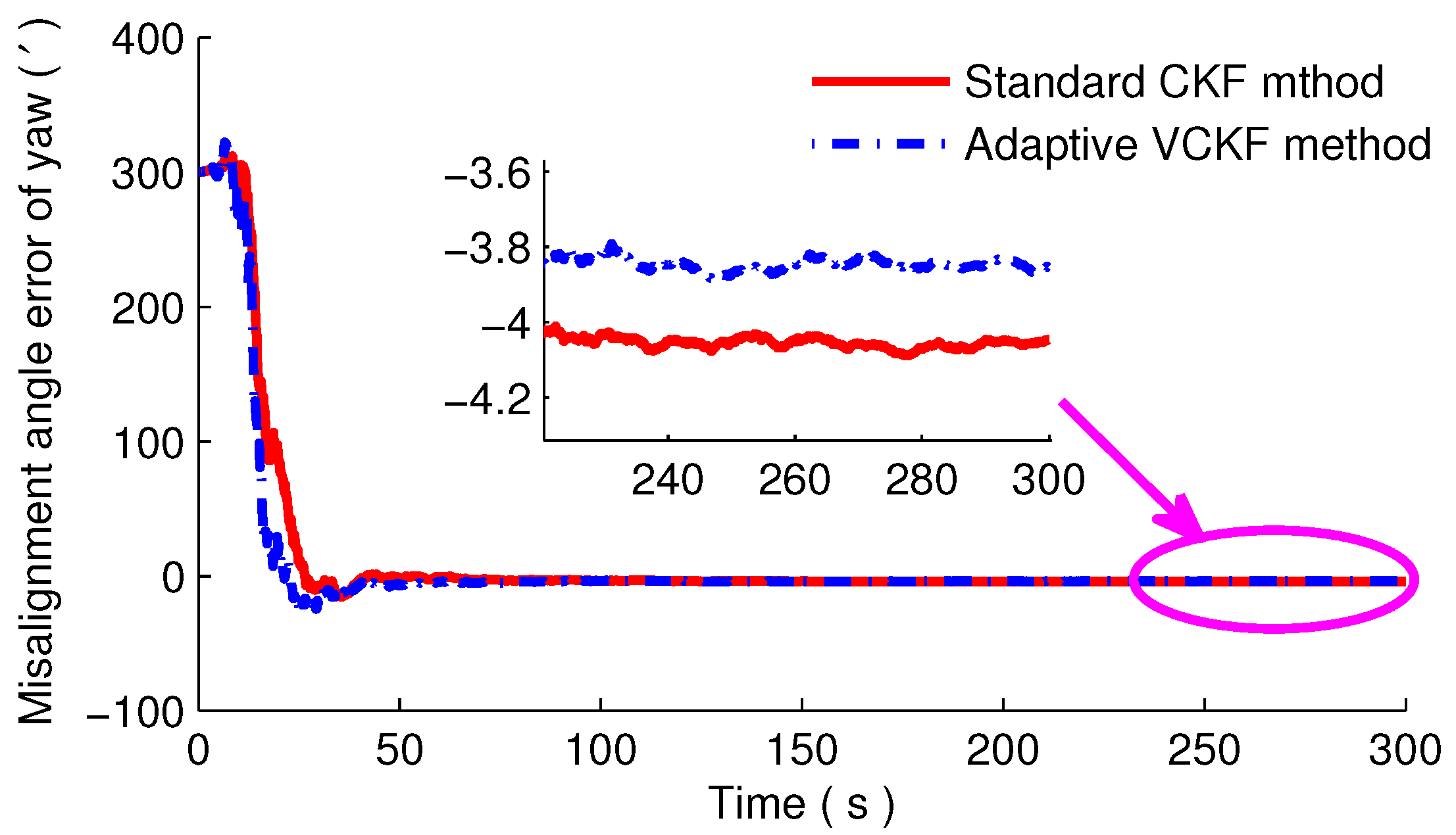
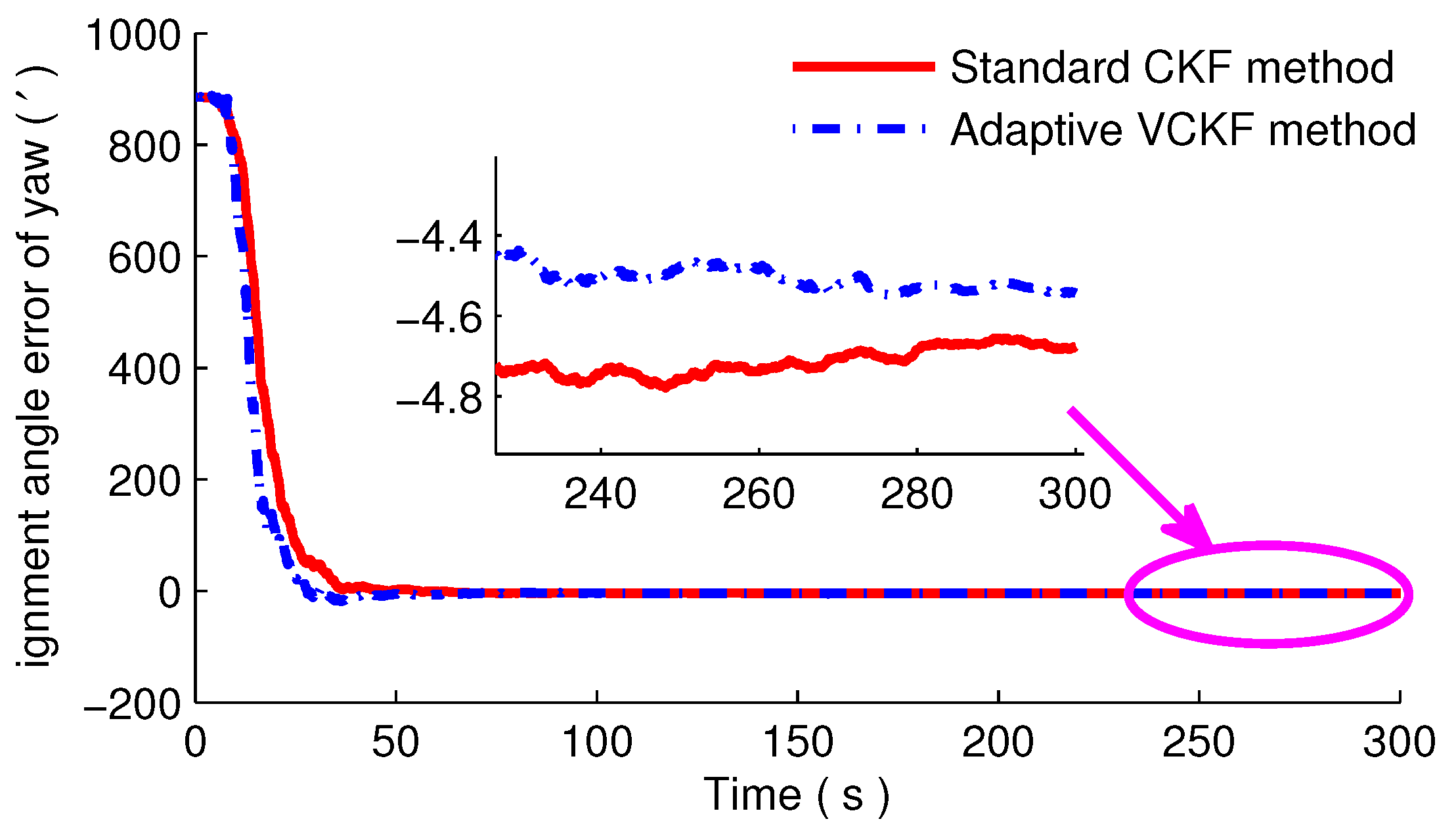
In Figure 1, the left, middle and right are the estimated results of Group 1, Group 2 and Group 3, respectively. It is obvious that the horizontal misalignment angles are nearly the same, not only in convergence speed, but also in estimated accuracy, so we pay more attention to the yaw angle. From Figure 2, Figure 3 and Figure 4, it is easy to see that the convergence rate and the estimated accuracy are different with these two filters. In the first 50 s, it is clear that the convergence rate of the adaptive VCKF method is faster than that of the standard CKF method.
To present the estimated accuracy more clearly, we magnify the purple region in the figures, and the estimated errors of yaw angles are listed in Table 2. It is clear that the estimated result with the adaptive VCKF method is still relatively better. That is because the system noise vector is estimated with the adaptive VCKF method, so the estimated states are closer to the true states than the one with the standard CKF.
4.2. Experiment and Analysis
To further validate the performance of the proposed initial alignment algorithm based on the adaptive VCKF method, experiments are carried out in Zhanjiang, China, as well. In this experiment, a ship was sailing with “Z-shaped” maneuvering, and the sailing trajectory of the ship is shown as in Figure 5. The whole experiment lasts 50 min. The schematic of the experimental setup and sensors is shown in Figure 6. In this experiment, the SINS developed by our own lab is fixed on the mounting-base in the cabin, closed to the high-accuracy inertial navigation system PHINS manufactured by ixBlue Company, France. Additionally, the NavQuest 600 DVL is installed at the bottom of the ship. The performance parameters of sensors are detailed in Table 3.
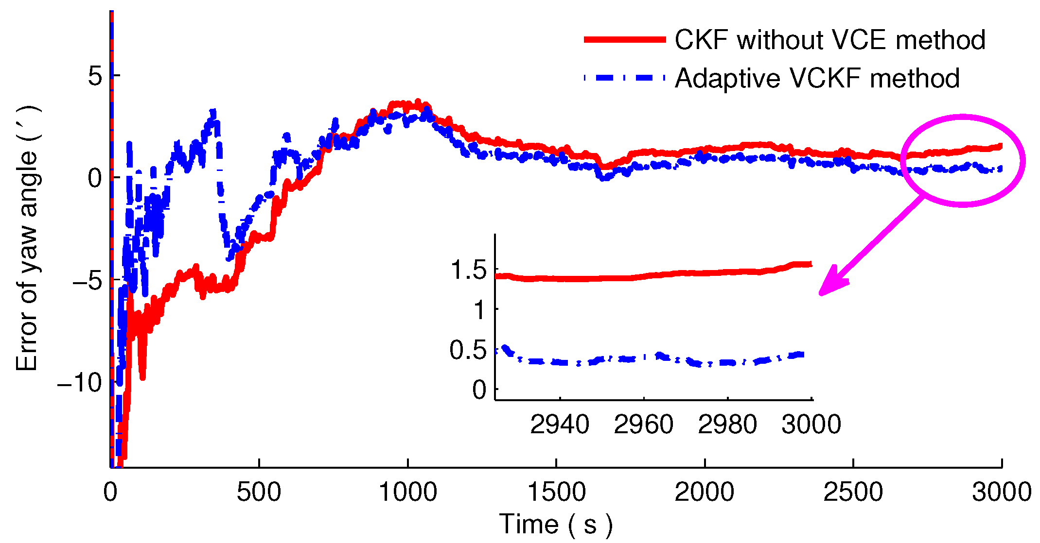
It is known from [29] that the heading and attitude accuracy of PHINS when it works with GPS is good enough. Therefore, the navigation information from PHINS is utilized as the reference to evaluate the performance of the novel initial alignment algorithm. Since the differences of horizontal errors with the normal CKF and the adaptive CKF based on VCE are nearly the same, we only analyze the yaw angle, as shown in Figure 7.
In Figure 7, the red solid line and the blue dotted line represent the estimated results with the normal CKF and the adaptive VCKF method, respectively. It is obvious that the blue line converges to zero rapidly in 400 s, although the trend is almost the same as the red line. Additionally, final estimated results are 1.55 and 0.43 with the standard CKF method and the adaptive VCKF method, respectively. Therefore, an estimation result closer to the actual value is obtained with the proposed filter without a priori knowledge about the system noise.
5. Conclusions
In order to solve the nonlinearity and uncertainty problems of initial alignment in the SINS/DVL integrated system of AUVs, a novel nonlinear and adaptive filter, named VCKF, was proposed based on the CKF and VCE methods in this paper. The main focus of this manuscript was establishing a nonlinear system model of the SINS/DVL integrated navigation system and deriving the CKF and VCE methods. On the basis of this, we presented the adaptive VCKF method combining these two method’s merits. To verify the effectiveness of the novel initial alignment algorithm, simulations and experiments were carried out, and the results showed that an estimation result closer to the actual value is obtained with the proposed filter without a priori knowledge about the system noise in the SINS/DVL integrated navigation system of AUVs.
Acknowledgments
This paper is funded by the International Exchange Program of Harbin Engineering University for Innovation-oriented Talents Cultivation, the National Natural Science Foundation of China (Grant Nos. 51509049, 51679047, 51379047), the Natural Science Foundation of Heilongjiang Province, China (Grant No. F201345), the Fundamental Research Funds for the Central Universities of China (Grant No. GK2080260140), the National key foundation for exploring scientific instrumentof China (Grant No. 2016YFF0102806) and the Postdoctoral Foundation of Heilongjiang Province (No. LBH-Z16044).
Author Contributions
Qianhui Dong and Yibing Li conceived of and designed the experiments. Ya Zhang performed the experiments. Qianhui Dong and Ya Zhang analyzed the data. Qian Sun and Ya Zhang wrote the paper.
Conflicts of Interest
The authors declare no conflict of interest.
References
- Paull, L.; Saeedi, S.; Seto, M.; Li, H. AUV navigation and localization: A review. IEEE J. Ocean. Eng. 2014, 39, 131–149. [Google Scholar] [CrossRef]
- Li, W.; Wang, J.; Lu, L.; Wu, W. A Novel Scheme for DVL-Aided SINS In-Motion Alignment Using UKF Techniques. Sensors 2013, 13, 1046–1063. [Google Scholar] [CrossRef] [PubMed]
- Zhu, D.; Li, W.; Yan, M.; Yang, S.X. The path planning of AUV based on DS information fusion map building and bio-inspired neural network in unknown dynamic environment. Int. J. Adv. Robot. Syst. 2014, 11, 34. [Google Scholar] [CrossRef]
- Li, D.; Ji, D.; Liu, J.; Lin, Y. A multi-model EKF integrated navigation algorithm for deep water AUV. Int. J. Adv. Robot. Syst. 2016, 13, 1–15. [Google Scholar] [CrossRef]
- Chang, L.; Li, J.; Chen, S. Initial Alignment by Attitude Estimation for Strapdown Inertial Navigation Systems. IEEE Trans. Instrum. Meas. 2015, 64, 784–794. [Google Scholar] [CrossRef]
- Tan, C.; Zhu, X.; Su, Y.; Wang, Y.; Wu, Z.; Gu, D. A New Analytic Alignment Method for a SINS. Sensors 2015, 15, 27930–27953. [Google Scholar] [CrossRef] [PubMed]
- Dorveaux, E.; Boudot, T.; Hillion, M.; Petit, N. Combining inertial measurements and distributed magnetometry for motion estimation. In Proceedings of the American Control Conference (ACC), San Francisco, CA, USA, 29 June–1 July 2011; pp. 4249–4256. [Google Scholar]
- Gao, W.; Deng, L.; Yu, F.; Zhang, Y.; Sun, Q. A novel initial alignment algorithm based on the interacting multiple model and the Huber methods. In Proceedings of the 2016 IEEE/ION Position, Location and Navigation Symposium (PLANS), Savannah, GA, USA, 11–14 April 2016; pp. 910–915. [Google Scholar]
- Han, S.; Wang, J. A Novel Initial Alignment Scheme for Low-Cost INS Aided by GPS for Land Vehicle Applications. J. Navig. 2010, 63, 663–680. [Google Scholar] [CrossRef]
- Xiong, J.; Guo, H.; Yang, Z. A two-position SINS initial alignment method based on gyro information. Adv. Space Res. 2014, 53, 1657–1663. [Google Scholar] [CrossRef]
- Hu, Z.; Su, Y. Initial alignment of the MEMS inertial measurement system assisted by magnetometers. In Proceedings of the 2016 31st Youth Academic Annual Conference of Chinese Association of Automation (YAC), Wuhan, China, 11–13 November 2016; pp. 276–280. [Google Scholar]
- Gao, W.; Zhang, Y.; Wang, J. A Strapdown Interial Navigation System/Beidou/Doppler Velocity Log Integrated Navigation Algorithm Based on a Cubature Kalman Filter. Sensors 2014, 14, 1511–1527. [Google Scholar] [CrossRef] [PubMed]
- Sun, G.; Zhu, Z.H. Fractional-Order Tension Control Law for Deployment of Space Tether System. J. Guid. Control Dyn. 2014, 37, 157–167. [Google Scholar] [CrossRef]
- Atia, M.M.; Liu, S.; Nematallah, H.; Karamat, T.B.; Noureldin, A. Integrated Indoor Navigation System for Ground Vehicles With Automatic 3-D Alignment and Position Initialization. IEEE Trans. Veh. Technol. 2015, 64, 1279–1292. [Google Scholar] [CrossRef]
- Ali, J.; Mirza, M.R.U.B. Initial orientation of inertial navigation system realized through nonlinear modeling and filtering. Measurement 2011, 44, 793–801. [Google Scholar] [CrossRef]
- Han, H.; Xu, T.; Wang, J. Tightly Coupled Integration of GPS Ambiguity Fixed Precise Point Positioning and MEMS-INS through a Troposphere-Constrained Adaptive Kalman Filter. Sensors 2016, 16, 1057. [Google Scholar] [CrossRef] [PubMed]
- Athans, M.; Wishner, R.; Bertolini, A. Suboptimal state estimation for continuous-time nonlinear systems from discrete noisy measurements. IEEE Trans. Autom. Control 1968, 13, 504–514. [Google Scholar] [CrossRef]
- Haykin, S. Chapter 7: The Unscented Kalman Filter; John Wiley & Sons, Inc.: Hoboken, NJ, USA, 2002; pp. 221–280. [Google Scholar]
- Sun, G.; Zhu, Z.H. Fractional-Order Dynamics and Control of Rigid-Flexible Coupling Space Structures. J. Guid. Control Dyn. 2015, 38, 1324–1329. [Google Scholar] [CrossRef]
- Arasaratnam, I.; Haykin, S. Cubature Kalman Filters. IEEE Trans. Autom. Control 2009, 54, 1254–1269. [Google Scholar] [CrossRef]
- Arasaratnam, I.; Haykin, S.; Hurd, T.R. Cubature Kalman Filtering for Continuous-Discrete Systems: Theory and Simulations. IEEE Trans. Signal Process. 2010, 58, 4977–4993. [Google Scholar] [CrossRef]
- Wang, J.G.; Gopaul, N.; Scherzinger, B. Simplified Algorithms of Variance Component Estimation for Static and Kinematic GPS Single Point Positioning. J. Glob. Position. Syst. 2009, 8, 43–52. [Google Scholar] [CrossRef]
- Zhang, L. Robust H-infinity CKF/KF hybrid filtering method for SINS alignment. IET Sci. Meas. Technol. 2016, 10, 916–925. [Google Scholar] [CrossRef]
- Narasimhappa, M.; Rangababu, P.; Sabat, S.L.; Nayak, J. A modified Sage-Husa adaptive Kalman filter for denoising Fiber Optic Gyroscope signal. In Proceedings of the 2012 Annual IEEE India Conference (INDICON), Kochi, India, 7–9 December 2012; pp. 1266–1271. [Google Scholar]
- Jin, M.; Zhao, J.; Jin, J.; Yu, G.; Li, W. The adaptive Kalman filter based on fuzzy logic for inertial motion capture system. Measurement 2014, 49, 196–204. [Google Scholar] [CrossRef]
- Chang, L.; Li, K.; Hu, B. Huber’s M-estimation-based process uncertainty robust filter for integrated INS/GPS. IEEE Sens. J. 2015, 15, 3367–3374. [Google Scholar] [CrossRef]
- Wang, R.; Xiong, Z.; Liu, J.Y.; Li, R.; Peng, H. SINS/GPS/CNS information fusion system based on improved Huber filter with classified adaptive factors for high-speed UAVs. In Proceedings of the 2012 IEEE/ION Position, Location and Navigation Symposium (PLANS), Myrtle Beach, SC, USA, 23–26 April 2012; pp. 441–446. [Google Scholar]
- Yu, F.; Sun, Q.; Lv, C.; Ben, Y.; Fu, Y. A SLAM Algorithm Based on Adaptive Cubature Kalman Filter. Math. Probl. Eng. 2014, 2014, 1–11. [Google Scholar] [CrossRef]
- Available online: http://www.ixblue.com/products/phins/ (accessed on 18 July 2017).
Figure 1.
The estimation of horizontal misalignment angles. The red solid line denotes the estimated results with the standard cubature Kalman filter (CKF) method, while the blue dashed line is the estimated results with the adaptive CKF and the adaptive variance components estimation (VCE) filter (VCKF) method. The upper three figures are the misalignment errors of the pitch angle, and the bottom three figures are the misalignment errors of the roll angle.
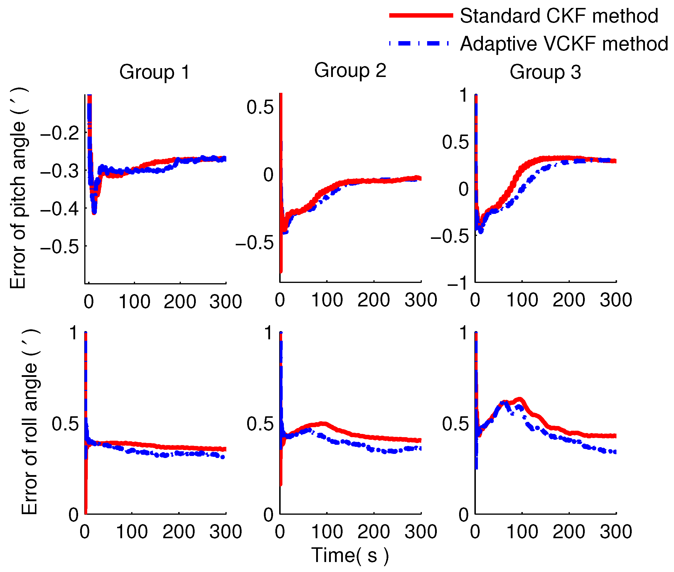
Figure 2.
The first group estimation results of the yaw angle. The red solid line denotes the estimated result with the standard CKF method, while the blue dashed line is the estimated results with the adaptive VCKF method.
Figure 2.
The first group estimation results of the yaw angle. The red solid line denotes the estimated result with the standard CKF method, while the blue dashed line is the estimated results with the adaptive VCKF method.

Figure 3.
The second group estimation results of the yaw angle. The red solid line denotes the estimated results with the normal CKF without the VCE method, while the blue dashed line is the estimated results with the adaptive CKF based on the VCE method.
Figure 3.
The second group estimation results of the yaw angle. The red solid line denotes the estimated results with the normal CKF without the VCE method, while the blue dashed line is the estimated results with the adaptive CKF based on the VCE method.
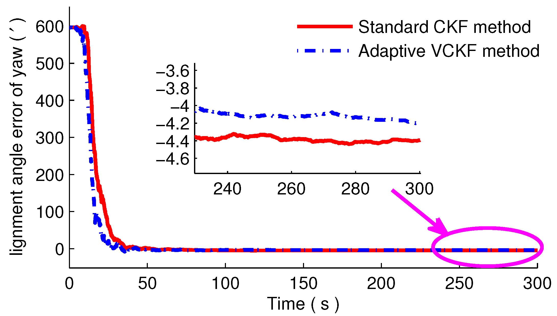
Figure 4.
The third group estimation results of the yaw angle. The red solid line denotes the estimated result with the standard CKF method, while the blue dashed line denotes the estimated result with the adaptive VCKF method.
Figure 4.
The third group estimation results of the yaw angle. The red solid line denotes the estimated result with the standard CKF method, while the blue dashed line denotes the estimated result with the adaptive VCKF method.

Figure 5.
The ship’s real trajectory with the “Z-shape”. The red line is the sailing trajectory, while the purple triangle and the cyan rectangle are the initial position and the end position, respectively.
Figure 5.
The ship’s real trajectory with the “Z-shape”. The red line is the sailing trajectory, while the purple triangle and the cyan rectangle are the initial position and the end position, respectively.
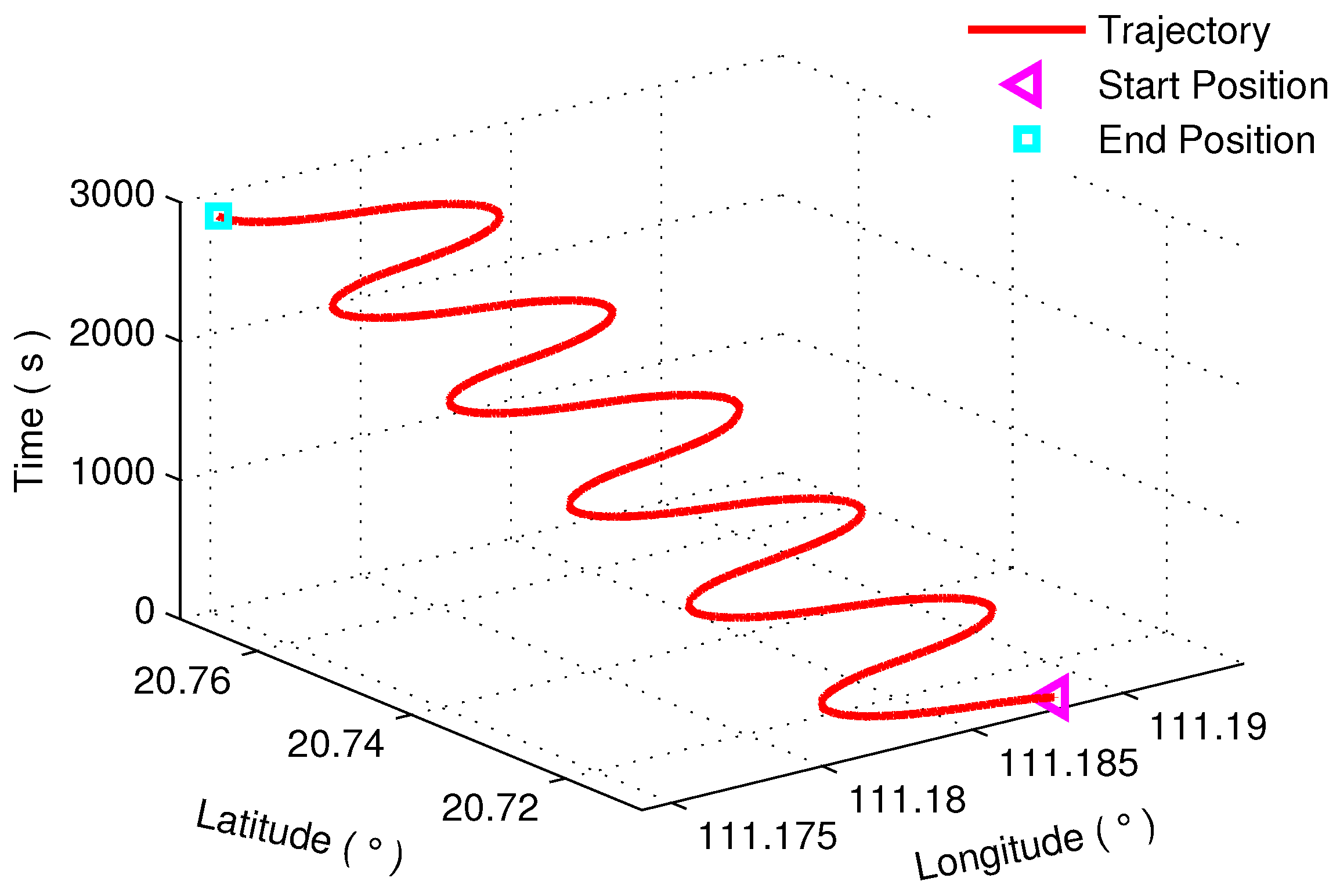
Figure 6.
The ship and installed sensors in this experiment. The upper right is the inertial systems, SINS (the black one) and PHINS (the blue one); the bottom right is the DVL.
Figure 6.
The ship and installed sensors in this experiment. The upper right is the inertial systems, SINS (the black one) and PHINS (the blue one); the bottom right is the DVL.
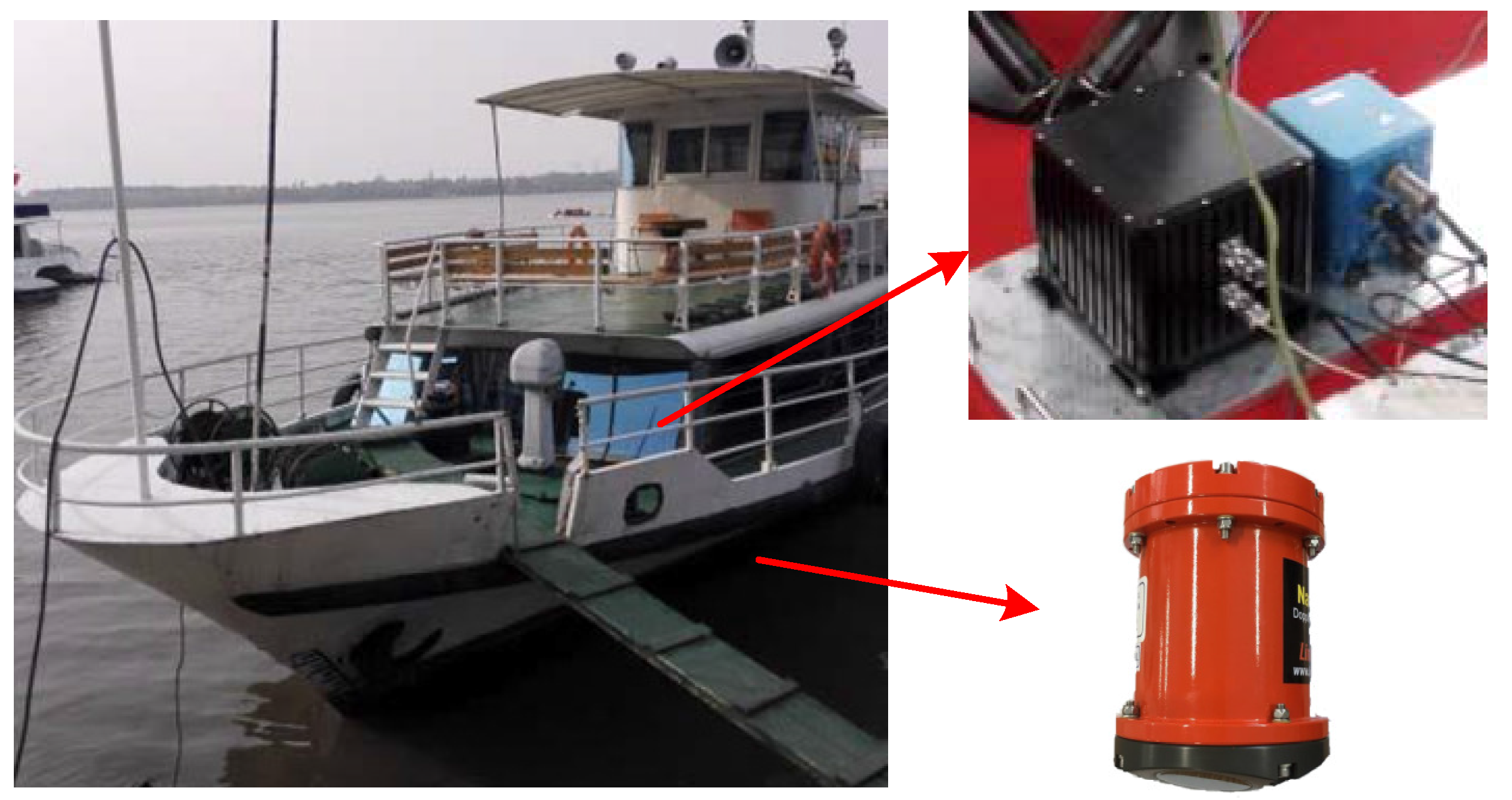
Figure 7.
The estimated error of yaw angles. The red solid line and the blue dashed line are the estimated results with normal CKF and improved CKF based on VCE, respectively. To present the estimated accuracy more clearly, we magnify the purple region.
Figure 7.
The estimated error of yaw angles. The red solid line and the blue dashed line are the estimated results with normal CKF and improved CKF based on VCE, respectively. To present the estimated accuracy more clearly, we magnify the purple region.

Table 1.
Simulation parameters.
| Parameters | Sets |
|---|---|
| Initial latitude | |
| Initial longitude | |
| Initial horizontal velocity | m/s |
| Gravity acceleration | m/s |
| Initial horizontal misalignment angles | |
| Initial vertical misalignment angles | Group 1: ; |
| Group 2: ; | |
| Group 3: ; | |
| Constant biases of the accelerometers | |
| Random noise of the accelerometers | |
| Constant drifts of the gyroscopes | /h |
| Random noise of the gyroscopes | /h |
| Sampling frequency | 100 Hz |
Table 2.
Simulation results of estimated yaw angle error.
| Groups | Error of Yaw Angle () | |
|---|---|---|
| CKF without VCE Method | Adaptive VCKF Method | |
| Group 1 | −4.05 | −3.86 |
| Group 2 | −4.40 | −4.19 |
| Group 3 | −4.71 | −4.54 |
Table 3.
Key performance of inertial sensors and DVL.
| Parameters | Values | |
|---|---|---|
| Gyroscope | Dynamic range | /s |
| Bias stability | /h | |
| random walk | /h | |
| Scale factor stability | 50 ppm | |
| Accelerometer | Dynamic range | g |
| Bias stability | mg | |
| random walk | mg | |
| Scale factor stability | 50 ppm | |
| DVL | Frequency | 600 kHz |
| Accuracy | mm/s | |
| Maximum Altitude | 110 m | |
| Minimum Altitude | 0.3 m | |
| Maximum Velocity | kn | |
| Maximum Ping Rate | 5/s |
© 2017 by the authors. Licensee MDPI, Basel, Switzerland. This article is an open access article distributed under the terms and conditions of the Creative Commons Attribution (CC BY) license (http://creativecommons.org/licenses/by/4.0/).
Share and Cite
MDPI and ACS Style
Dong, Q.; Li, Y.; Sun, Q.; Zhang, Y. An Adaptive Initial Alignment Algorithm Based on Variance Component Estimation for a Strapdown Inertial Navigation System for AUV. Symmetry 2017, 9, 129. https://doi.org/10.3390/sym9080129
AMA Style
Dong Q, Li Y, Sun Q, Zhang Y. An Adaptive Initial Alignment Algorithm Based on Variance Component Estimation for a Strapdown Inertial Navigation System for AUV. Symmetry. 2017; 9(8):129. https://doi.org/10.3390/sym9080129
Chicago/Turabian StyleDong, Qianhui, Yibing Li, Qian Sun, and Ya Zhang. 2017. "An Adaptive Initial Alignment Algorithm Based on Variance Component Estimation for a Strapdown Inertial Navigation System for AUV" Symmetry 9, no. 8: 129. https://doi.org/10.3390/sym9080129
Note that from the first issue of 2016, this journal uses article numbers instead of page numbers. See further details here.