Structural Controls on Copper Mineralization in the Tongling Ore District, Eastern China: Evidence from Spatial Analysis


1
School of Resources and Environmental Engineering, Jiangxi University of Science and Technology, Ganzhou 341000, China
2
Jiangxi Key Laboratory of Mining Engineering, Jiangxi University of Science and Technology, Ganzhou 341000, China
3
Institute of Multipurpose Utilization of Mineral Resources, CAGS, Chengdu 610041, China
4
College of Earth Sciences, Chengdu University of Technology, Chengdu 61005, China
5
School of Water Resource and Environment, China University of Geosciences, Beijing 341515, China
*
Author to whom correspondence should be addressed.
Minerals 2018, 8(6), 254; https://doi.org/10.3390/min8060254
Submission received: 4 May 2018
/
Revised: 11 June 2018
/
Accepted: 14 June 2018
/
Published: 15 June 2018
(This article belongs to the Special Issue Structural Control of Mineral Deposits: Theory and Reality)
Abstract
:Structures exert significant controls on hydrothermal mineralization, although such controls commonly have cryptic expression in geological datasets dominated by 2D maps. Analysis of spatial patterns of mineral deposits and quantification of their correlation with detailed structural features are beneficial to understand the plausible structural controls on mineralization. In this paper, a series of GIS-based spatial methods, including fractal, Fry, distance distribution and weights-of-evidence analyses, were employed to reveal structural controls on copper mineralization in the Tongling ore district, eastern China. The results indicate that Yanshanian intrusions exert the most significant control on copper mineralization, followed by EW-trending faults, intersections of basement faults and folds. The scale-variable distribution patterns of copper occurrences are attributed to the different structural controls operating in the basement and sedimentary cover. In the basement, EW-trending faults serve as pathways for channeling Yanshanian magma from a deep magma chamber to structurally controlled trap zones in the caprocks, imposing an important regional control on the spatial distribution of Cretaceous magmatic-hydrothermal system genetically related to copper mineralization. In the sedimentary cover, bedding-parallel shear zones, formed during the progressive folding and shearing in Indosinian and overprinted by tensional deformation in Yanshanian, act as favorable sites for hosting, focusing and depositing the ore-bearing fluids, playing a vital role in the localization of stratabound deposits at fine scale.
1. Introduction
Structural controls on hydrothermal mineralization at various scales have been widely recognized [1,2,3,4,5]. At a global scale, hydrothermal systems usually form in specific tectonic settings, e.g., porphyry systems mostly occur in magmatic arc settings [1,2,3]. At a regional scale, hydrothermal deposits show close proximity to regional faults system or shear zones, which sever as pathways for transporting ore-forming fluids from deep-seated sources to shallow depositing spots [6,7]. At a deposit scale, hydrothermal replacement disseminations, breccias and veins, which are related to subsidiary fracture zones of regional structures, serve as favorable sites for focusing and depositing the ore-bearing fluids and are interpreted to be responsible for localization of orebodies [7]. However, such controls may usually have cryptic expression in various sources of geological records, because (i) structures, especially large-scale structures, may have variable expressions from depth to surface (e.g., mylonite zone at depth and fault zone near the surface) [7]; (ii) spatial associations between map-generalized structures and surface-projected deposits in 2D maps may lead to an inaccurate view or even misunderstanding with respect to controls of mineralization; and (iii) structural features together with structurally controlled mineralization may be formed through successive deformation and polyphase tectonics [8]. Thus, it is a challenge to identify ore-related structural features and elucidate structural controls, as well as measure their contributions to the formation of mineral deposits.
GIS-based spatial analysis has been well-established and developed in the last three decades, assisting in identification of inherent patterns of ore-related geological features and delineation of interplay of the processes that constrain the formation of mineral deposits [9,10,11,12]. More specifically, with the help of quantitative methods and easy-to-use GIS software, delineating the spatial patterns of known occurrences of mineral deposits and their associations with geological features (e.g., structural, lithological and geochemical features) can, in addition to field observations, geochemical and mineralogical laboratory methods, provide insights into the controlling mechanisms operating at different scales [10,13,14,15], especially in the brownfield areas where a relatively large number of mineral deposits have been well-explored [15]. Furthermore, recognition of geological features controlling the mineralization is critical for defining exploration criteria in future prospecting [16].
Since mineral occurrences are simplified to be represented as points on large-scale maps in various applications of spatial analyses, methods of spatial analysis for point patterns have been increasingly employed in studying spatial distribution and geological controls of mineral deposits, mostly involving fractal geometry [17,18] and Fry analysis [19,20]. Through statistical calculation, fractal and Fry analyses are able to highlight the distribution pattern of mineral deposits that may be difficult to be recognized by exclusively relying on visual interpretation [5]. Moreover, distance distribution [14,21] and weights-of-evidence (WofE) analyses [22,23] can further quantify the strength of the spatial association between mineral deposits and geological features believed to be favorable in predicting the location of the mineralization. A joint application of these methods is necessary as individual methods only characterizes a particular aspect, such as non-random clustering of deposits or preferential direction of deposits distribution, of complex spatial features of mineralization systems [10,24].
The Tongling ore district (TOD) is one of the most important Cu producers in China, with totally estimated reserves of over 5 Mt copper [25]. Large stratabound copper deposits constitute the majority of the copper reserves in this area, e.g., the Donggushan deposit with 1 Mt Cu @ 1.01% [26] and the Xinqiao deposit with 0.5 Mt Cu @ 0.71% [27], which have attracted many studies focusing on their genesis [28,29,30,31,32,33,34,35,36]. These stratabound deposits were firstly considered to be of SEDEX origin by many researchers because of their stratiform orebodies and massive sulfide ores, and the major orebodies occurring in the Carboniferous strata were thought to be products of Late Paleozoic (Hercynian) sedimentary exhalative system [28,29,30]. Some researchers further proposed an exhalative origin overprinted by Yanshanian magmatic-hydrothermal processes, based on the restricted occurrences of the stratabound orebodies in areas where Yanshanian intrusions are particularly extensive [31,32,33]. In contrast, some authors advocated that the stratabound mineralization is of epigenetic origin and genetically associated with the Jurassic-Cretaceous tectono-thermal events [34,35,36]. The precise geochronological data derived from recent studies confirmed that the massive sulfide and skarn orebodies were coeval with the Yanshanian intrusions [25,27,37], supporting the magmatic-hydrothermal origin of these stratabound deposits.
Although the genesis of stratabound deposits is still disputable, most of the researchers tend to agree with the epigenetic origin or at least the dominant contribution of Yanshanian magmatic-hydrothermal activities in the superimposed ore-forming processes [38,39]. In the magmatic-related genetic model, the stratiform orebodies were formed as a result of progressive fluid-rock interaction along the bedding-parallel structurally controlled conduits and were integral but distal parts of a large hydrothermal system that produced the proximal skarn orebodies at the contact zones and porphyry orebodies in the Yanshanian intrusions [35]. Such hydrothermal system and stratabound deposits are similar to their counterparts elsewhere [35], among which the porphyry-skarn polymetallic deposits in the Ertsberg district of Indonesia and manto-type copper deposits in Chile are two representative examples. In the Ertsberg district, the Ertsberg East skarn orebody, one of the largest orebodies, is hosted by a bedding-parallel fault-bounded zone between the limestone of the Faumai Formation and dolomitic carbonate of the Waripi Formation [40]. In the Punta del Cobre district in Chile, the stratabound tabular orebodies occur in the andesite breccia horizons between underlying massive andesite and overlying shale, while the sites of economic copper concentration appear to be controlled by faults [41]. Since structure is an important controlling factor of these stratabound deposits, some relevant studies have been conducted in the TOD, including the spatial patterns [34], deformation model [42] and formative process [43] of ore-controlling structures. However, these studies mostly focus on theoretical deduction and qualitative analysis, and lack quantitative analysis concerning detailed structural features. Hence, this paper attempts to delineate the structural controls by both qualitative and quantitative analytical methods, focusing on the structural controlling mechanisms operating at different scales, which can facilitate the understanding of the formation of copper deposits and provide criteria for future exploration in the TOD.
2. Materials and Methods
2.1. Study Area
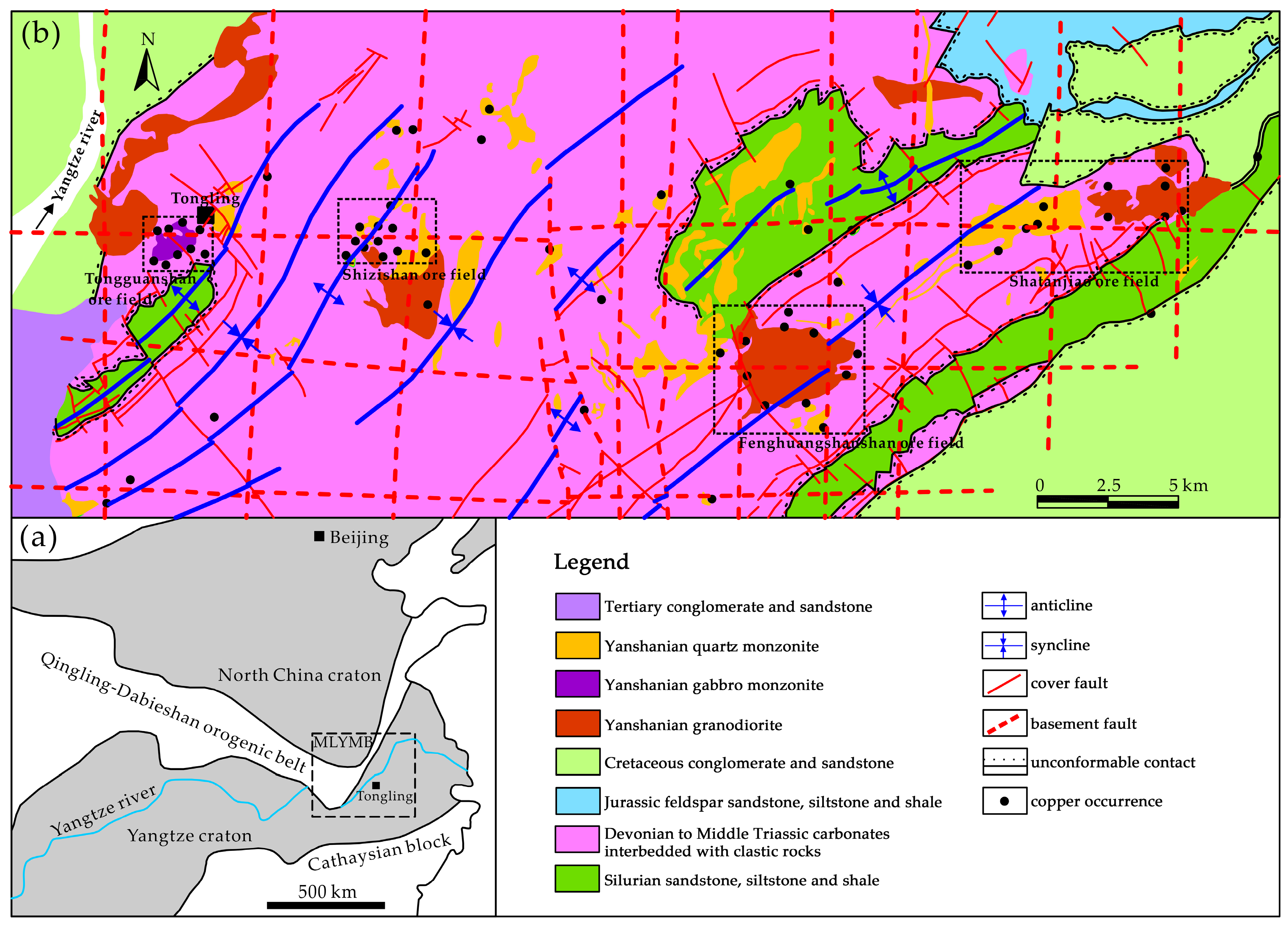
The TOD is situated in the central part of the Middle-Lower Yangtze Cu-Au-Fe metallogenic belt (MLYMB) along the Northern margin of the Yangtze craton, bordered by the Qingling-Dabieshan orogenic belt and the North China craton to the North (Figure 1a).
The Northern Yangtze craton is underlain by tonalitic-trondjhemitic-granitic (TTG) gneisses aged from 3.45 to 2.87 Ga [44]. The TTG gneisses and unconformably overlying Archean to Paleoproterozoic metamorphic rocks constituted the basement of the TOD [44]. From Cambrian to Middle Triassic, the TOD represented a stable trough filled with carbonate and clastic rocks of shallow marine facies [36]. Two sedimentary sequences developed in this period, including the Lower Silurian to Upper Devonian regressive bathyal to littoral clastic rocks and overlying Upper Carboniferous to Middle Triassic littoral to neritic carbonates interbedded with bathyal and alternative marine-continental clastic rocks [45]. The sedimentary strata were folded during the Indosinian movement which is initiated at the end of Middle Triassic due to the collision between the Yangtze craton and North China craton [35]. From Jurassic to Cretaceous, this region experienced an event that has long been interpreted as an intracontinental deformation stage with abundant magmatism [35,38,45], and developed thick terrestrial sedimentary and volcanic sequences which unconformably overlie the Silurian to Triassic strata. The detailed lithological description and contact relationship of sedimentary strata in the TOD are listed in Table 1.
The regional structures in the TOD are dominated by several folds with NE-striking axial surfaces and sigmoidal-shaped axes (Figure 1b). Secondary structures include NE-trending thrust faults, NW- and NNW-trending strike-slip faults [46]. The regional gravity anomalies [47] and deep seismic reflection profiles [48] indicate the presence of EW- and NS-trending basement faults. The Yanshanian magmatism resulted in more than 70 intrusions that are mainly composed of granodiorite, quartz monzonite, gabbro monzonite and their hypabyssal equivalents [26,49]. High-precision zircon U-Pb dating results have shown that the intrusions of this region were formed in the Early Cretaceous (mainly 145–129 Ma) [50,51]. The copper-polymetallic deposits discovered in the TOD are dominated by skarn-type, with minor porphyry-type copper deposits occurring in the deeper parts of some skarn deposits [45,50,51]. More than 60 copper-polymetallic skarn deposits and prospects have been discovered in the TOD, mainly clustering in four ore fields designated as Tongguanshan, Shizishan, Fenghuangshan and Shatanjiao ore field from west to east (Figure 1b).
The copper occurrences (including known deposits and prospects) and structural features employed in this study were derived from Geological Database of Bureau of Geological and Mineral Resources of Anhui Province based on 1:50,000 geological survey and complemented by the literature available for the study area concerning regional geological settings [26,42,45,49,51]. The raw data were examined before being inputted into a spatial database. Only those copper and copper-dominated polymetallic deposits were included in the analysis, since the other types of copper-related polymetallic deposits may be products of different structurally controlled processes when compared with copper mineralization. The structural features were reclassified into three categories including the basement faults, cover faults and folds. All the examined data were compiled to vector formats and imported into the ArcGIS 10 platform (Environmental Systems Research Institute, Redlands, CA, USA) for the subsequent spatial analyses.
2.2. Fractal Analysis
Fractals are entities that have similar geometrical patterns when observed in ranges of scales [17]. This scale-invariance can be depicted by a power-law proportional relationship between a measurement of the target pattern and its scale [17]. Various methods have been proposed for estimating the fractal dimension of a given pattern, each of which reveals an aspect of geometrical complexity of the target pattern [10,54]. The box-counting and radial-density methods, which are the most commonly used methods in analyzing geological point patterns, were employed to estimate corresponding fractal dimensions in this study. The fractal analysis can reveal the statistical scale-related laws of the distribution of copper occurrences, which may be products of structurally controlled processes.
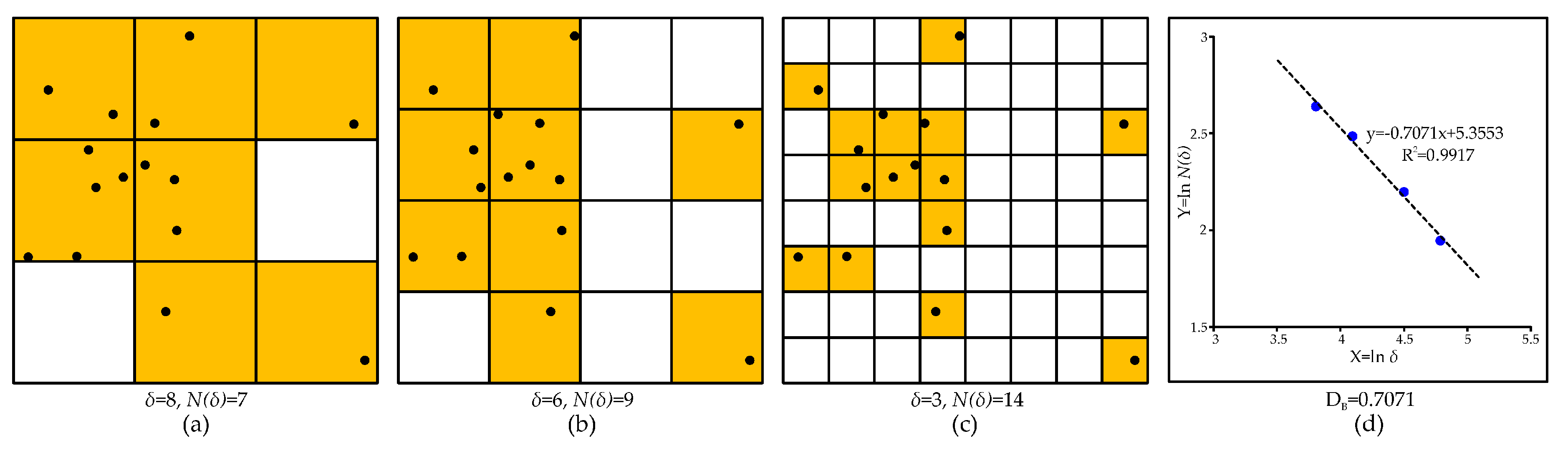
In the box-counting method, the study area involving geological features of interest (e.g., mineral deposits) is overlain by a grid that comprises square cells or boxes with side length δ, and then the number N(δ) of those boxes containing parts of target features is counted (Figure 2a). The above process is repeated using different box size δ to obtain corresponding box number N(δ) (Figure 2b,c). If the pattern under analysis pertains to fractal pattern, the relationship between N(δ) and δ should follow a power-law function as below [17]:
where DB is the box-counting fractal dimension, and A is a constant. Practically, a graph of log(N(δ)) versus log(δ) is plotted and then a best-fit regression line is drawn by the least square method, while the slope of the regression line represents the box-counting fractal dimension (Figure 2d).
In the radial-density method, fractal points, also called fractal dusts, have been demonstrated to satisfy a radial-density relationship, which can be described as [55]:
where, d is the average point density of the circles with a radius r that center in every point, and B is a constant, while DR is the radial-density fractal dimension. Likewise, DR is usually obtained by calculating the slope of a regression line that presents the linear relationship of d and r in a log-log plot.
2.3. Fry Analysis
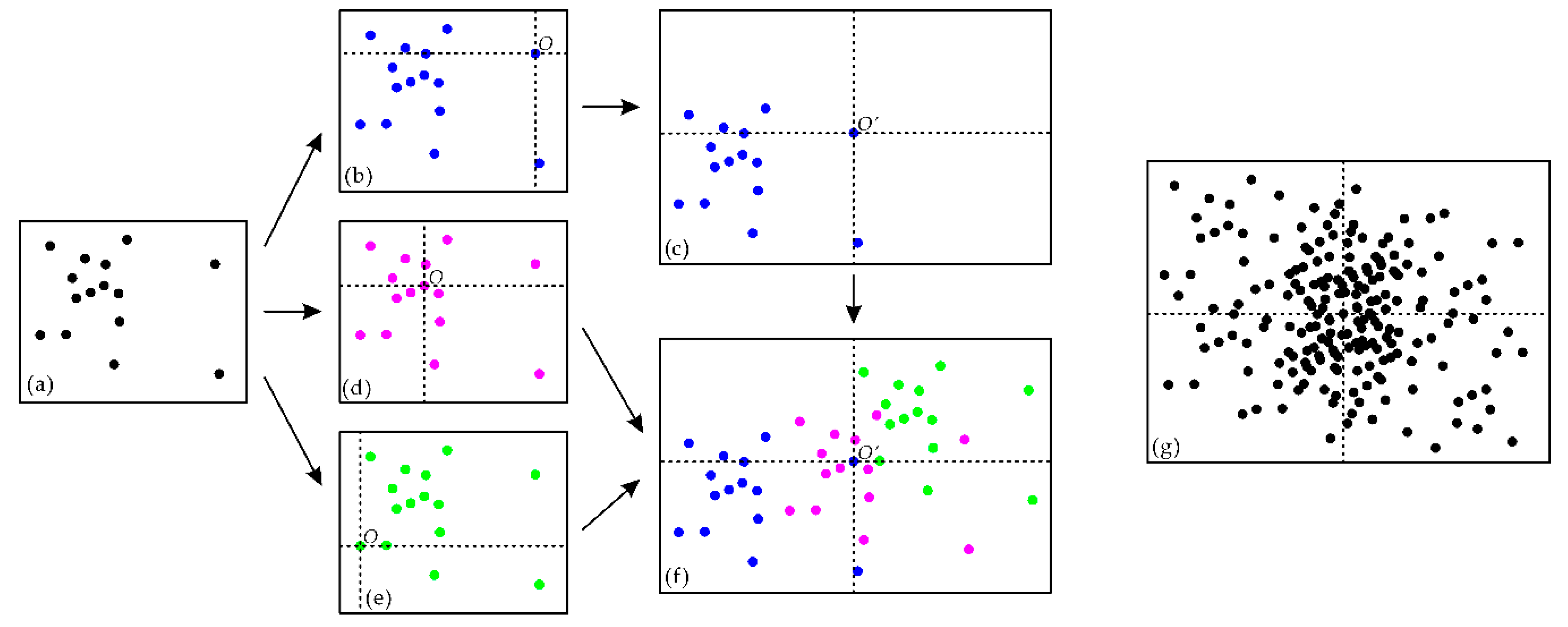
Fry analysis is a geometrical method of spatial autocorrelation for analyzing point patterns [22], which is implemented by the construction of an autocorrelation diagram called Fry plot. Figure 3 shows a basic procedure for creating Fry plot [10,24]: (i) two analogue sheets including an original sheet recording raw points (Figure 3a) and a blank tracing sheet are prepared; (ii) the origin of the original sheet O is placed on one of the raw points, thus preserving the orientations and distances of all the other points (Figure 3b); (iii) the points in the original sheet are then translated to the tracing sheet with O coinciding with the origin of the tracing sheet O’ (Figure 3c); (iv) the origin O moves to another raw point (Figure 3d), and the new distribution pattern of raw points is copied to the tracing sheet following step (iii) (Figure 3f). This procedure is repeated until every point in the original sheet is used as the origin O (Figure 3e,f), resulting in (n2-n) points in the tracing sheet for n raw points (Figure 3g). The final tracing sheet is termed as Fry plot, and the points in this sheet are called Fry points.
Fry plot records the distances and orientations of each raw point relative to every other point, thus enhancing subtle patterns of target point features [24], based on which rose diagrams are usually constructed to analyze preferential orientations of point pairs within specific distances that reveal the directional controls on mineralization at different map scales.
2.4. Distance Distribution Analysis
Distance distribution analysis is a spatially buffer-based method for quantifying spatial association between a set of points (i.e., mineral occurrences) and another set of spatial features [24,56]. This analysis involves calculating and comparing the cumulative relative frequency according to given distances from a certain set of geological features to (i) mineral occurrence locations (denoted as DM) and (ii) non-occurrence locations (denoted as DN). DN indicates naturally random probability density distribution of regular patterns within a given buffer distance, while DM presents a non-random probability density distribution of mineralized patterns that is characterized by unevenly clustering of mineral occurrences within the corresponding buffer. The difference D, which is calculated by (DM − DN), represents how much the cumulative frequency of mineral occurrences (i.e., DM) is higher or lower than that expected due to chance (i.e., DN), measuring the intensity of spatial association between the analyzed geological feature and mineralization.
In order to manifest statistically if DM is significantly greater than DN, an upper confidence band for the curve of DN (denoted as uc) can be given by [57]:
where M is the number of mineral occurrences that used to estimate DM, while N is the number of non-occurrence locations using for calculating DN, and 9.21 is a constant for significance level α = 0.01 [24].
2.5. Weights of Evidence (WofE) Analysis
The WofE analysis is a data-driven Bayesian statistical method that offers a quantitative measurement of spatial association between a set of given geological features and the target occurrences (e.g., mineral deposits, prospects or geological anomalies) [58,59].
A detailed mathematical explanation of the WofE method is available in Bonham-Carter (1994) [9]. In the GIS-based application of a mineral occurrence-related analysis, the WofE analysis is implemented on the basis of several binary predictor maps of geological features [9]. Firstly, the study area is subdivided into T square cells with an equal size, among which D cells are occupied by mineral occurrences. The prior probability can be defined as:
and the relative importance of spatial association between the geological feature Bi and mineralization is estimated by a pair of weights, namely positive weight W+ and negative weight W−, which can be given by:
where P denotes the corresponding probability; B and are the presence and absence of geological features; D and are the presence and absence of mineral occurrences. P(B|D), for example, represents the probability of B occurring given the presence of D. The contrast C is defined as an overall measurement of spatial correlation, which is given by:
In order to evaluate the significance of the contrast C, the confidence of the contrast (denoted as CS), obtained from a Student t-test, is employed here and defined as:
where S denotes the standard deviation of the corresponding parameter.
3. Results and Discussion
3.1. Spatial Patterns of Copper Occurrences
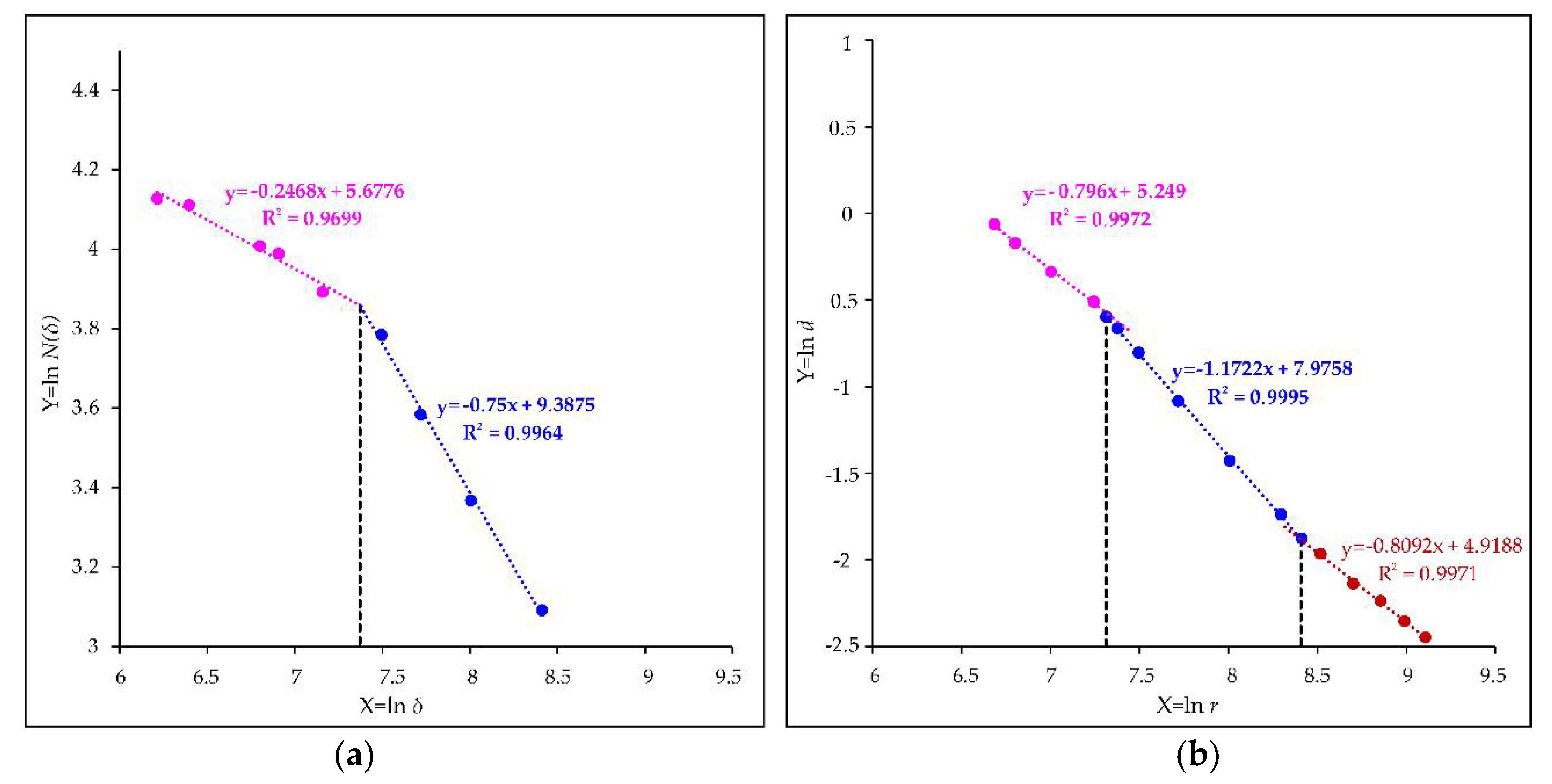
The box-counting log-log graph shows that the distribution of copper occurrences in the study area exhibits a bifractal pattern, i.e., the log-log plot of box number N(δ) versus box size δ can be fitted with two regression lines (Figure 4a), resulting in two fractal dimensions of 0.2468 (δ ≤ 1.6 km) and 0.75 (δ > 1.6 km). In contrast, the radial-density analysis yields a trifractal pattern, as indicated by three regression lines that represent three fractal dimensions varying from 0.796 (r ≤ 1.4 km), 1.1722 (between 1.5 and 4.5 km) to 0.8092 (r > 4.5 km) (Figure 4b). A single regression line represents a power-law (fractal) relationship between the measurements and their scales, implying a scale-invariance pattern resulted from a nonlinear process. In this study, the different fractal patterns of copper occurrences indicated by the multi-line fractal model could be ascribed to the different ore-controlling processes operating at different scales. It is noteworthy that the log-log graph, especially for radial-density analysis, seems to be alternatively fitted with one single regression line. However, the two-lines and three-lines fractal models shown in Figure 4 are assumed to be optimum because they reach the maximum regression coefficients (R2) of the fitted lines, meaning that the reduction of any regression line would lower the regression coefficients.
Although apparent differences in the fractal dimensions are noted in the above analyses, there is a general agreement between the result of box-counting method and that of radial-density analysis, such that variations in fractal dimensions, indicated by intersection of the neighbor regressing lines, both occur at around 1.5 km, suggesting that the different fractal structures exist within identical ranges (within 1.5 km and beyond 1.5 km) in both box-counting and radial-density fractal relationship. It is also noted that there is an intersection at 4.5 km in the radial-density fractal plot; however, it is not clear whether there also exists another fractal dimension in the box-counting analysis when taking box size greater than 4.5 km, since box number under such situation is not large enough to be statistically counted.
The results of fractal analyses in this study, including the multi-fractal dimension model and fractal structures occurring within identical ranges, are consistent with those of some previous studies [10,15,16,24]. It is considered that discrepancies in fractal dimensions are plausibly linked to different geological controls operating at diverse scales, e.g., regional-, local- and prospect-scale [10]. Nevertheless, such scale-variable geological controls are still cryptic and need to be delineated by further analysis.
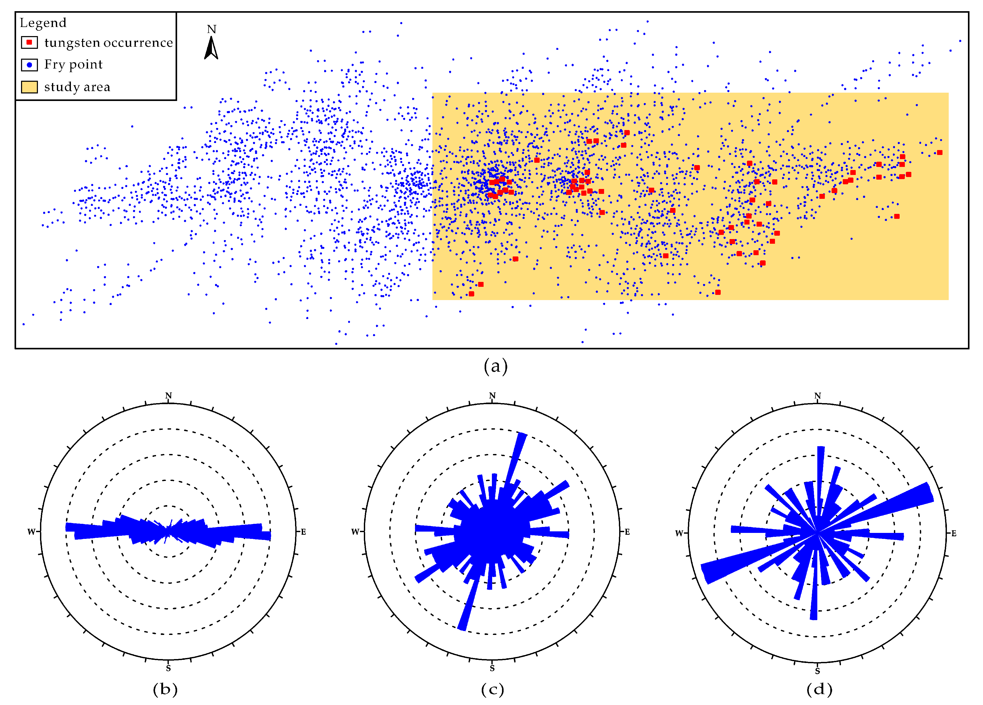
Fry analysis has been performed to investigate the orientations of plausible controls on copper mineralization. 3906 Fry points were delivered from 63 copper occurrences in the TOD (Figure 5a), based on which rose diagrams were constructed. The rose diagram for all Fry points illustrates a simply dominant EW trend (Figure 5b), suggesting a fundamental EW-trending control on copper mineralization at regional scale. Since fractal analyses indicate variations in fractal dimensions around 1.5 and 4.5 km, we also analyzed the characteristics of Fry points within these ranges. The rose diagram for Fry points within 4.5 km of each other indicates a preferential NNE trend, with subordinate NE and EW trends (Figure 5c). The rose diagram for Fry points within 1.5 km of each other exhibits a main NE-NEE trend, with subsidiary trends in EW and NS directions (Figure 5d).
The results of Fry analysis infer different directional controls at regional- (>4.5 km) and fine- (<4.5 km) scales, which could be correlated to detailed structural features in the TOD. However, such correlation is not specific. For example, the NE-trending control at fine scale may be related to the NE-trending faults or be linked to the folds with NE-striking axes. Further analysis is necessary so as to delineate the one-to-one correspondence between the scale-variable controls and detailed structural features.
3.2. Spatial Correlation of Structural Features with Copper Mineralization
Structural features are the outcomes of diverse geological processes, only a few of which are associated with ore-forming processes and sever as structural controls on mineralization [10,24]. In order to reveal the subtle structural controls in the TOD, the structural features were grouped in terms of their orientations, and the spatial associations of these features with copper mineralization were quantitatively assessed by distance distribution analysis. The study area was subdivided into 20,250 square cells with side length of 200 m, among which 63 cells containing copper occurrences represent occurrence samples and the other cells are taken as non-occurrence samples.
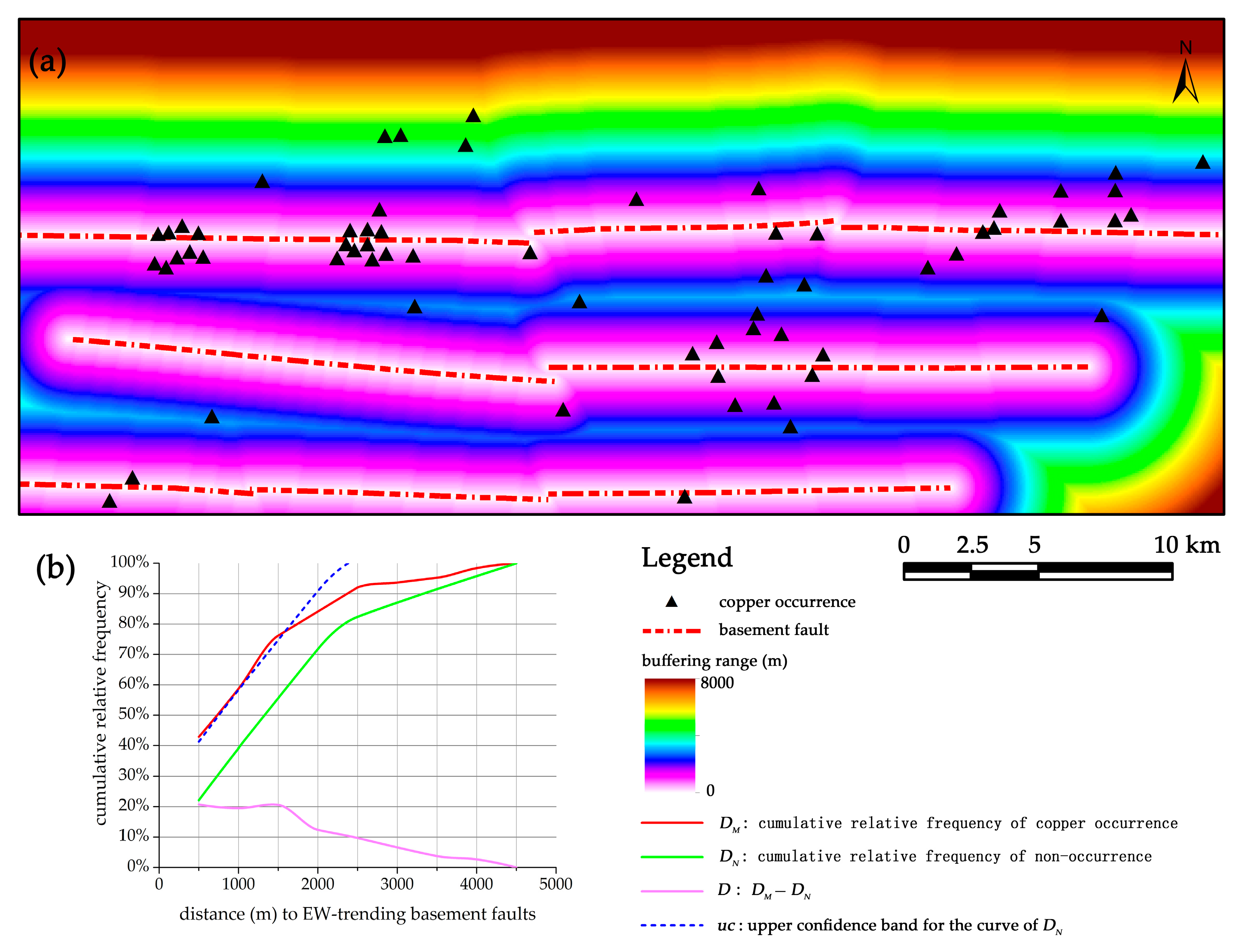
The EW-trending basement faults exhibit a positive correlation with copper occurrences according to the curve of D (Figure 6). Within an optimal buffer distance of 1.5 km, there is at most 21% higher frequency of copper occurrences than what would be expected due to chance. Such correlation is verified to be statistically significant (at α = 0.01) since the curve of DM is plotted above the upper confidence band of DN within a 1.5 km buffer (Figure 6b).
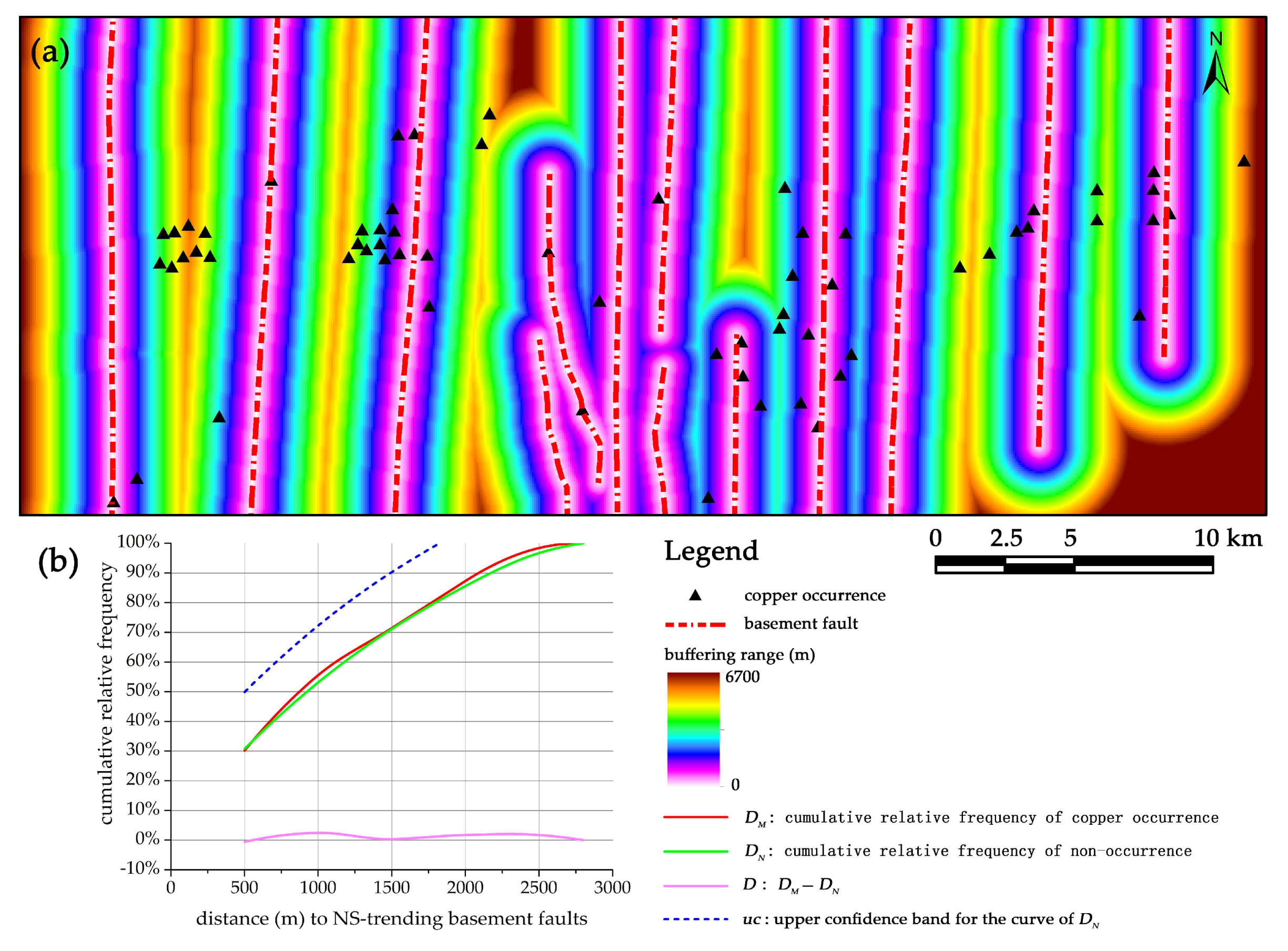
The NS-trending basement faults have a positive but weak association with copper occurrences beyond the buffer distance of 1 km, reaching only 2% higher frequency than what would be expected (Figure 7). However, the curve of DM is plotted below the upper confidence band of DN in the whole range of buffer analysis (Figure 7b), indicating that the weak association between NS-trending faults and copper mineralization is not of statistical significance.
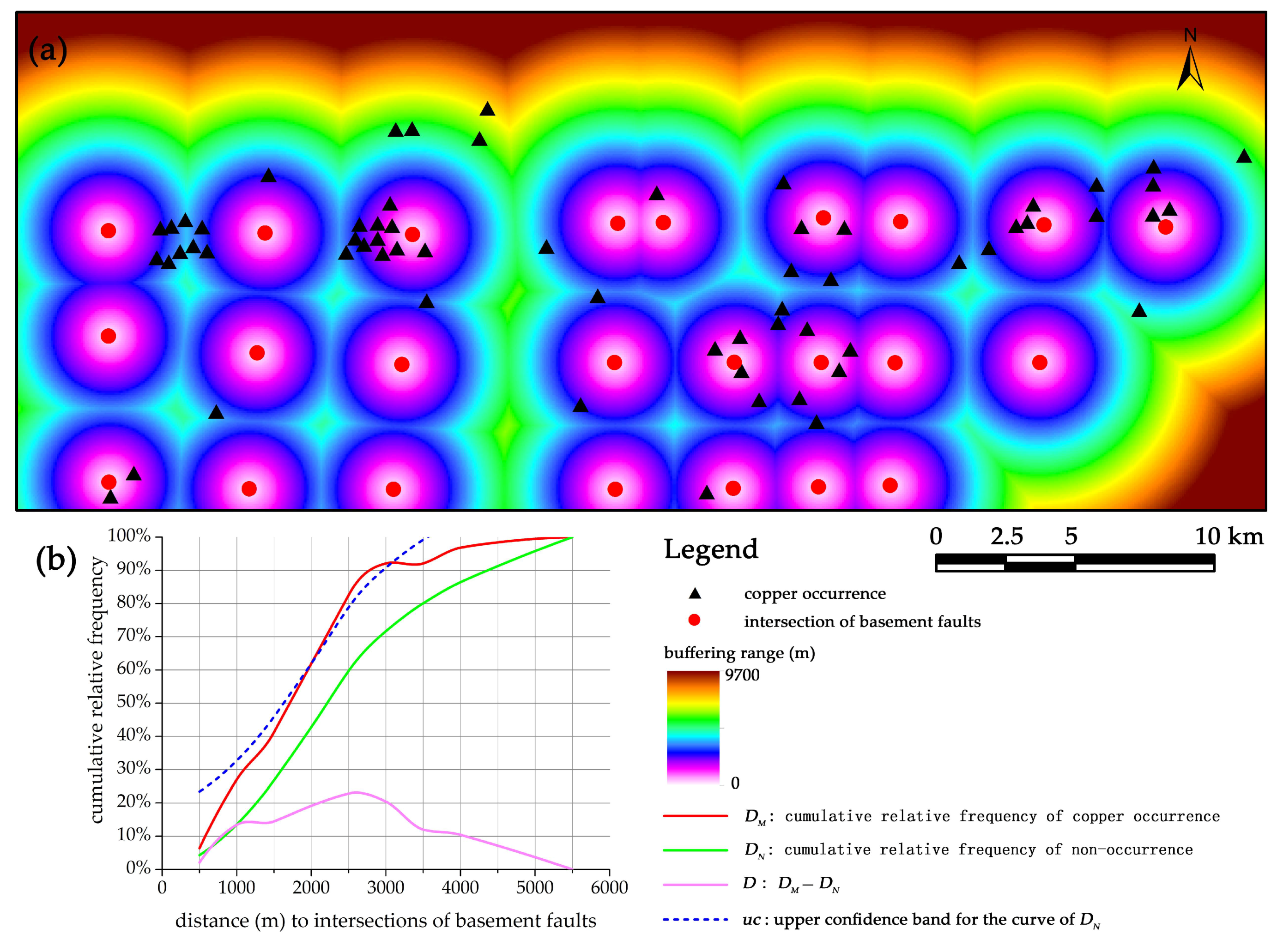
The intersections of the basements faults have a statistically significantly positive correlation with copper occurrences between the buffer distances of 2 and 3 km (Figure 8). At an optimal buffer distance of 2.5 km, there is 23% higher frequency of copper occurrences than what would be expected (Figure 8b).
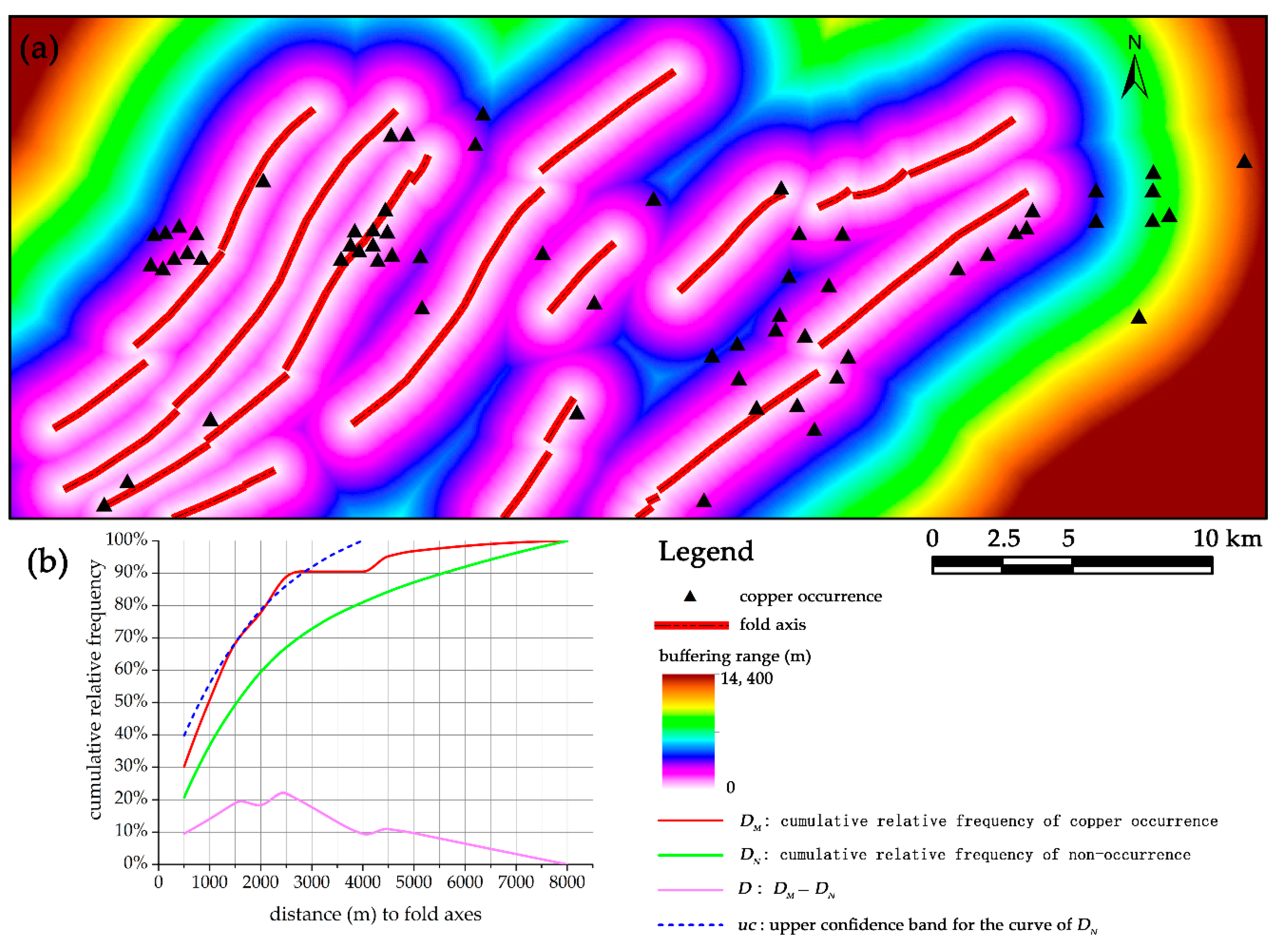
The folds exhibit a statistically significantly positive correlation with copper occurrences in the buffers ranging from 1.5 to 3 km (Figure 9). There is 22% higher frequency of copper occurrences than what would be expected at a 2.5 km buffer (Figure 9b).
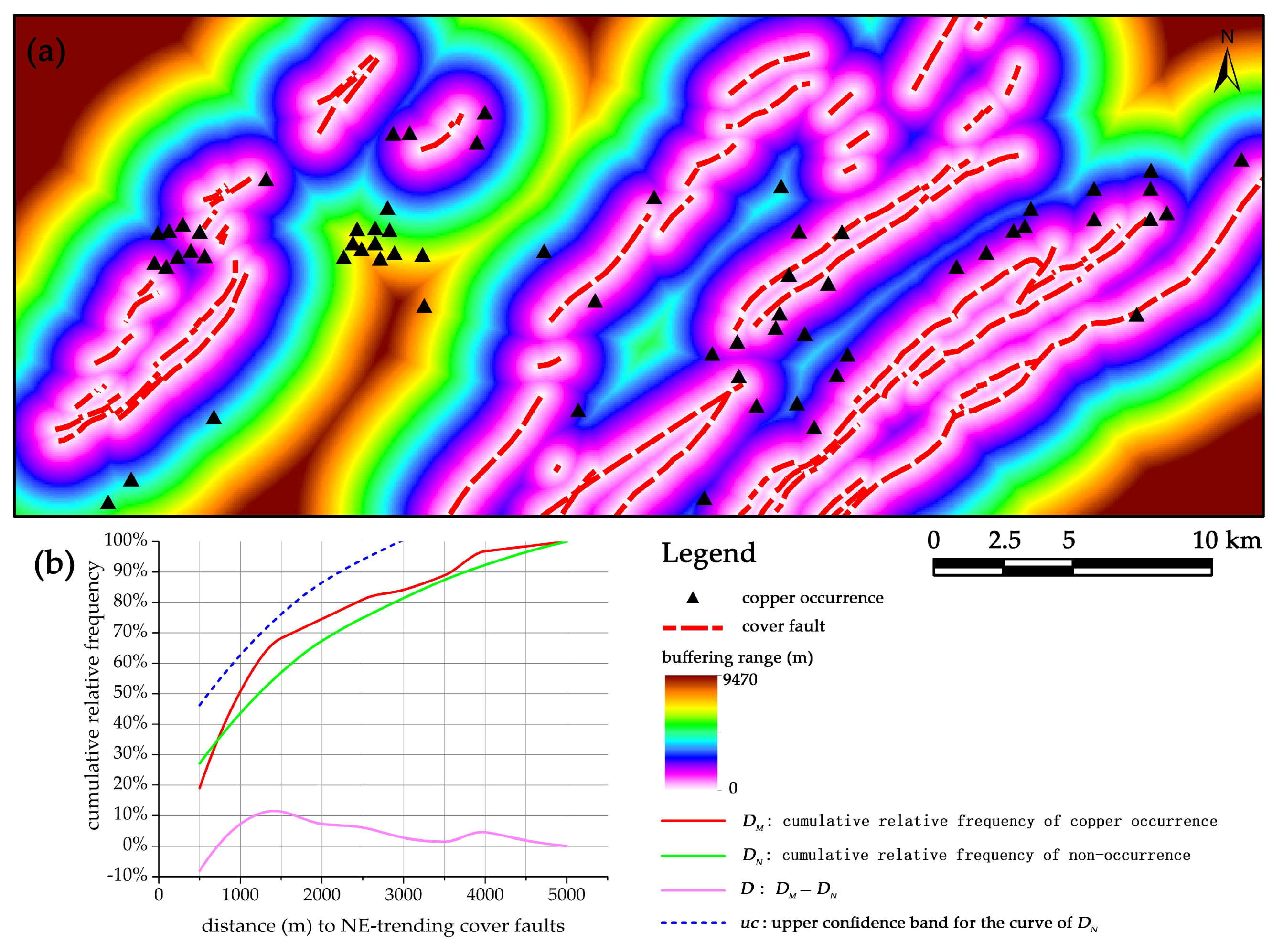
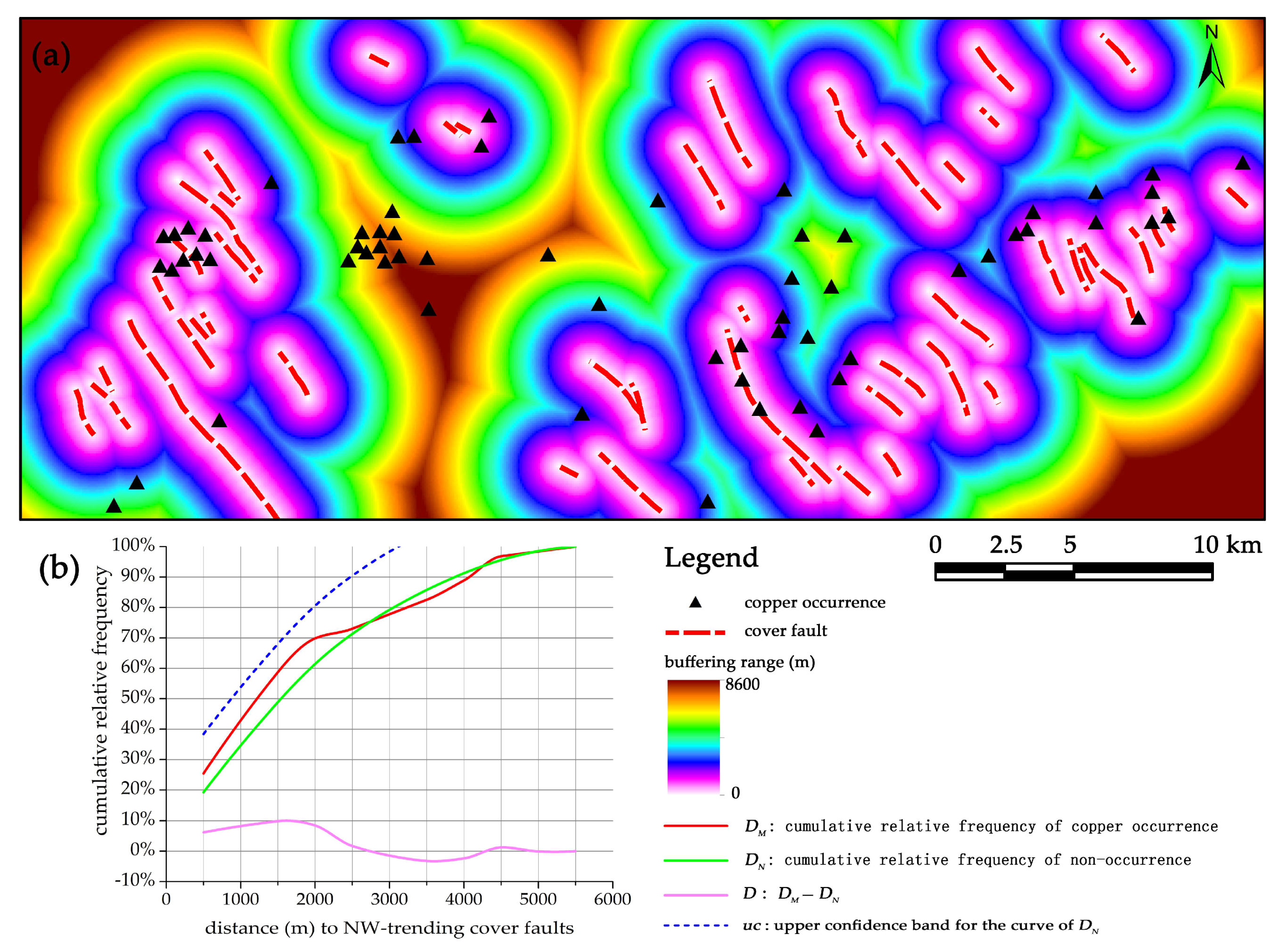
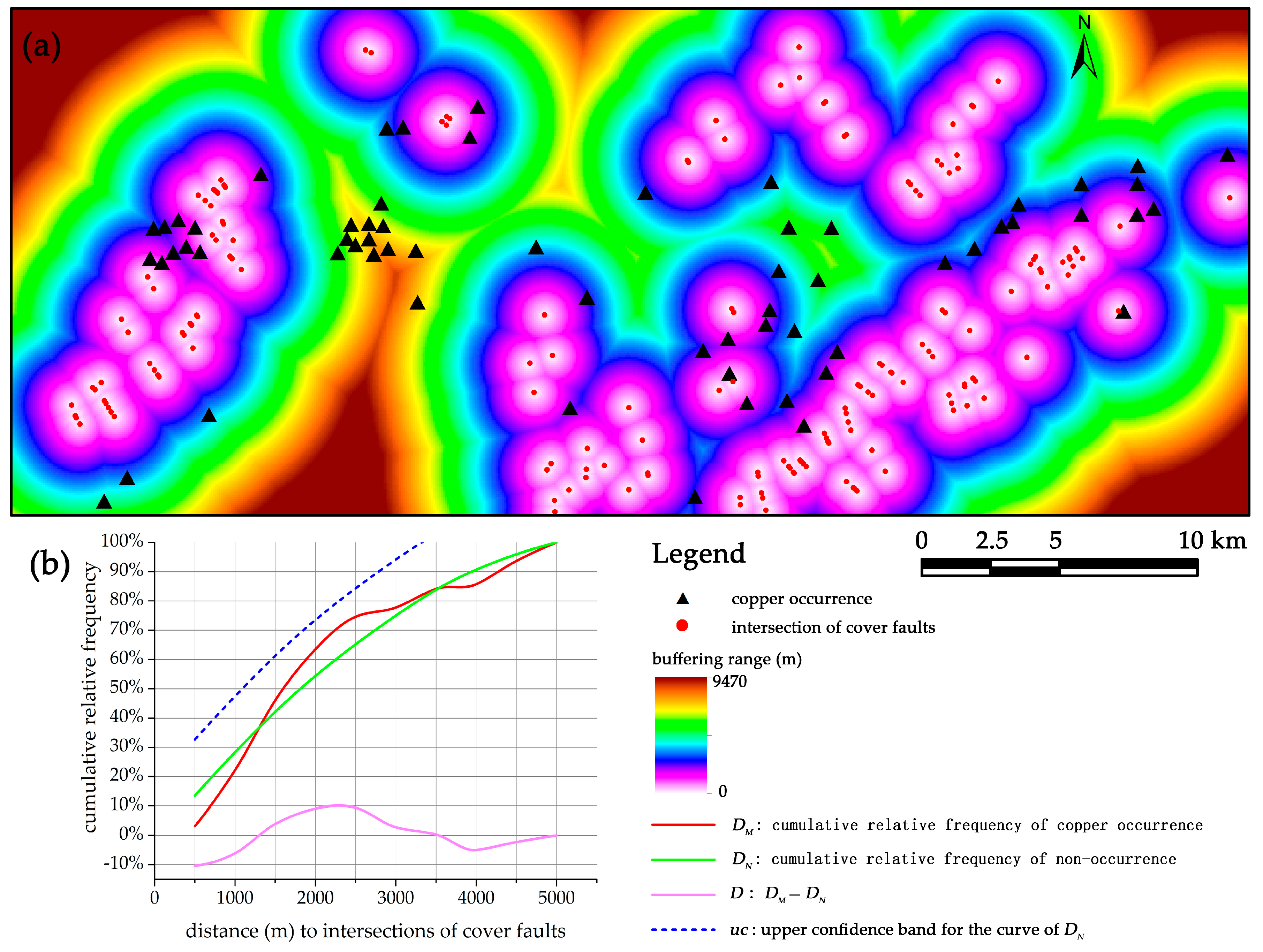
The cover faults consisting of NE- and NW-trending faults as well as the intersections of these faults show positive spatial association with copper occurrences. There are at most 11%, 10% and 9% higher frequencies of occurrences than what would be expected within the optimal buffers of NE-, NW-trending faults and their intersections, respectively (Figure 10, Figure 11 and Figure 12). Nevertheless, none of these structural features have a statistically significantly associated with copper occurrence at any buffer distance (Figure 10b, Figure 11b and Figure 12b).
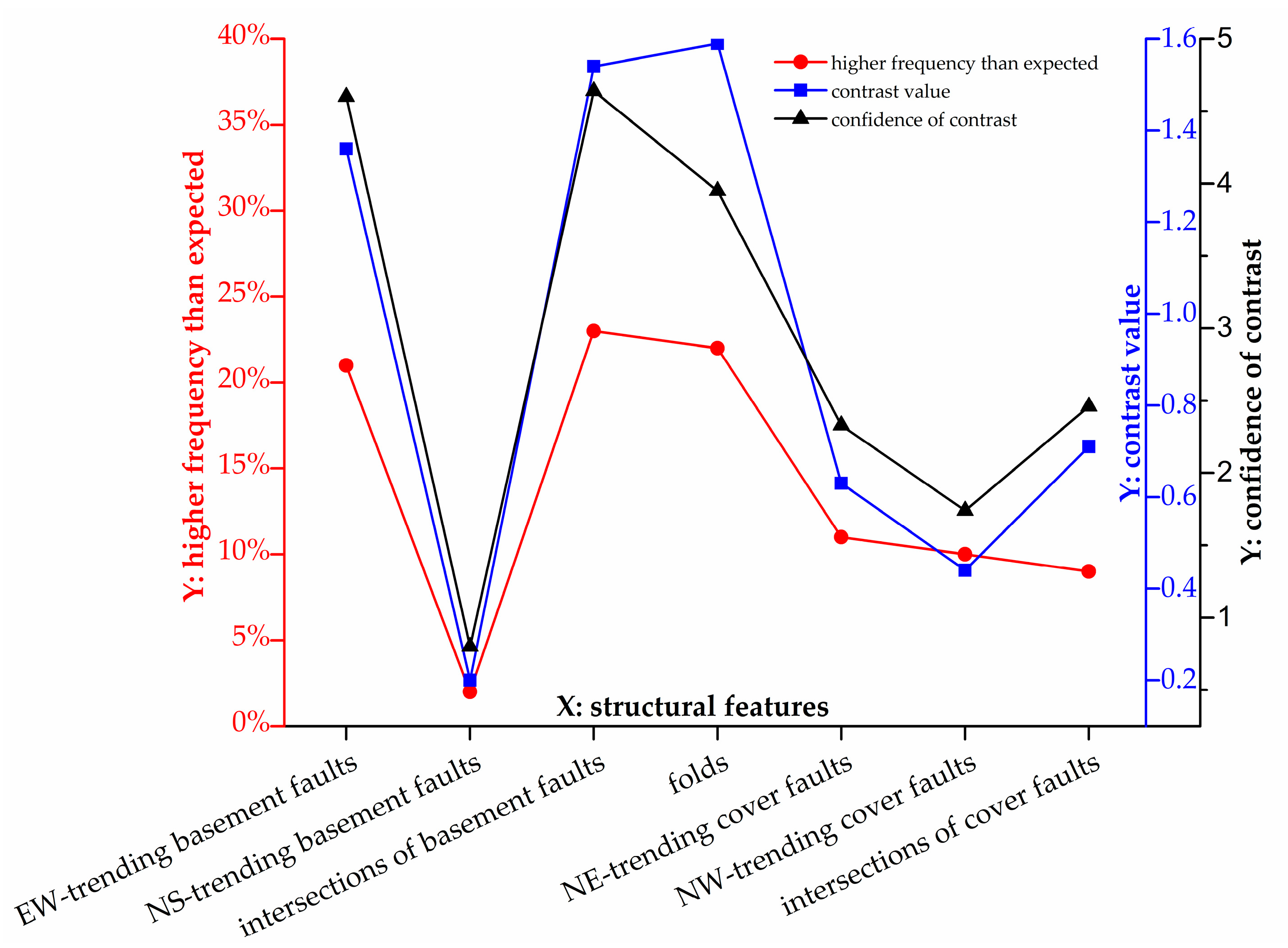
WofE analysis was also implemented to investigate the association of structural features with copper occurrences. At corresponding optimal buffer distances, the contrast values and confidences of contrast were calculated. As depicted in Figure 13 and Table 2, the EW-trending faults, intersections of basement faults and folds have top three highest values of both contrast and confidence of contrast, which are remarkably greater than those of the other structural features. The contrasts and confidences of contrast, which can assist in evaluating the intensity of spatial association, show exactly the same variations as the results derived from distance distribution analysis, implying that the EW-trending faults, intersections of basement faults and folds are plausibly major structural controls on copper mineralization in the TOD.
3.3. Spatial Correlation of Faults with Intrusions
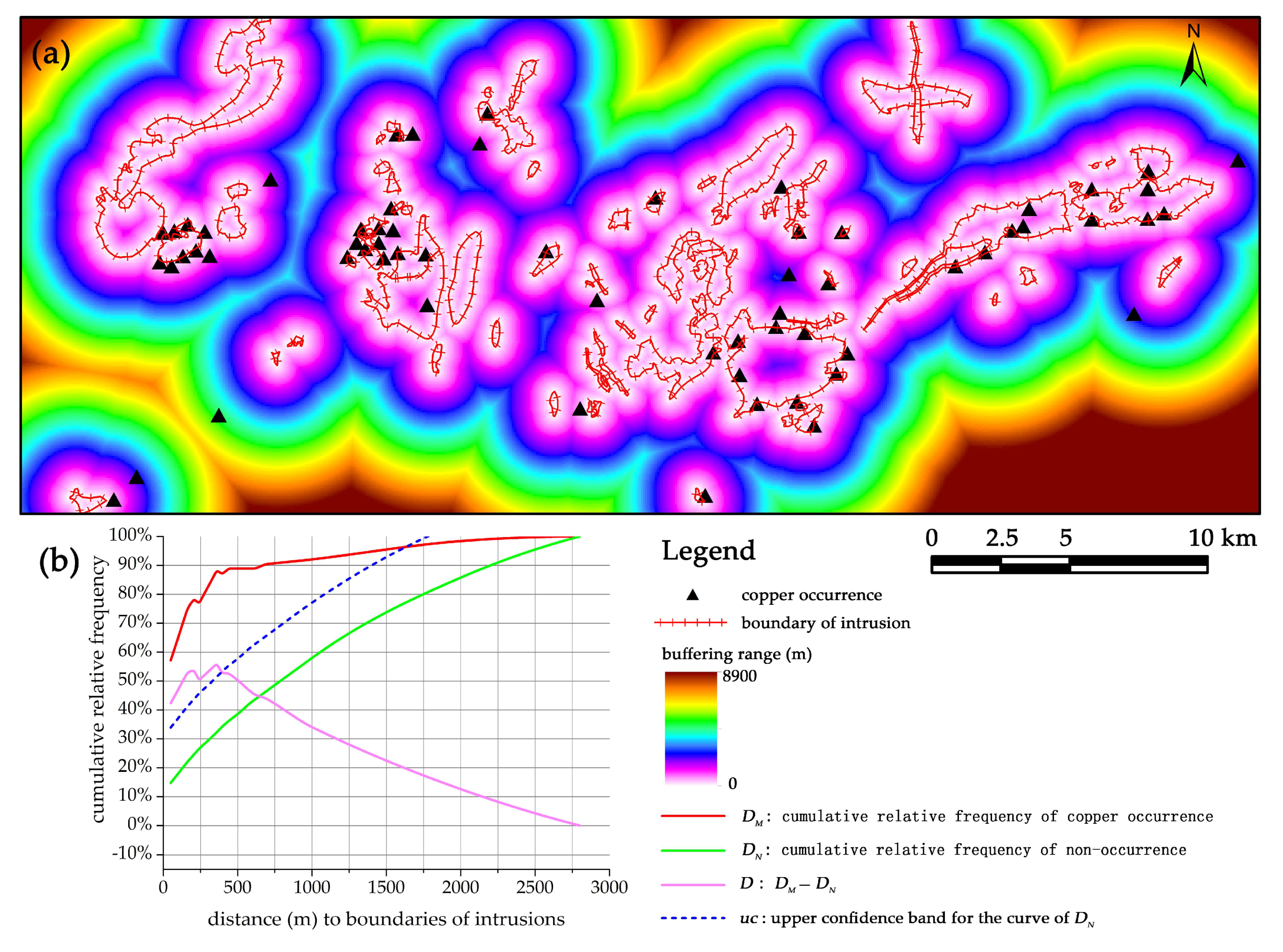
Considering that copper deposits in the TOD are dominated by skarn-type, Yanshanian intrusion is a key ore-controlling factor and its contact with wall rock can be considered as a special structure. The result of distance distribution analysis shows the strongest association of the contact with copper occurrences. Within a 1.7 km buffer of the contact, there is at most 55% higher frequency of copper occurrences than what would be expected, and such strong association is manifested to be statistically significant (Figure 14). The WofE analysis yields a contrast value of 3.04 and a confidence value of 8.03 which are markedly higher than the corresponding values of the other structural features (Table 2), supporting the most significant association of the contact with copper mineralization.
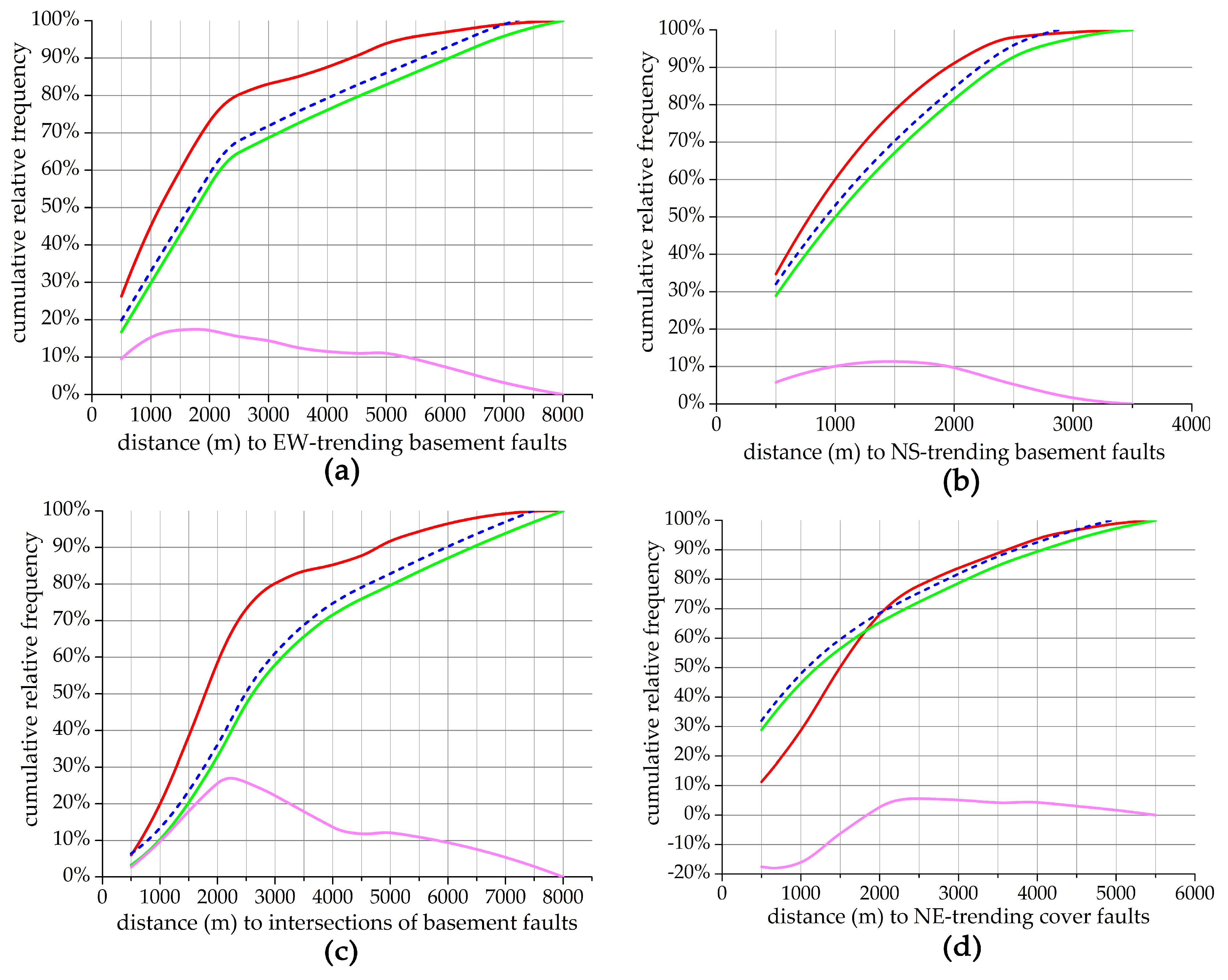
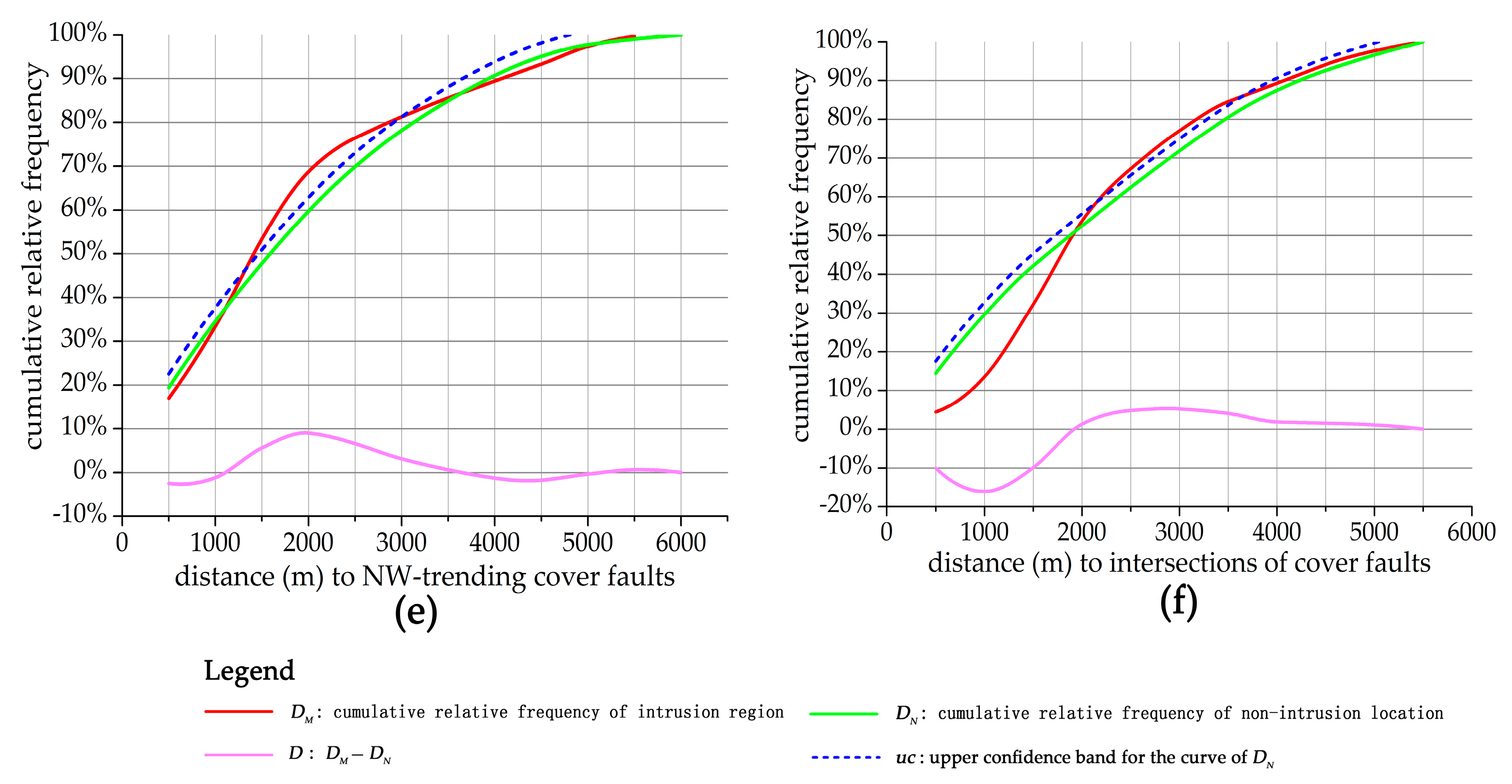
Since regional faults are considered to control the emplacement of intrusions according to many previous studies [45,48,50], we also performed distance distribution analysis to investigate the correlation of intrusion with the faults of various orientations. The results show that the EW-, NS-trending faults and their intersections have statistically significantly positive correlations with intrusion regions at most of the buffer distances (Figure 15a–c). There are 26% and 17% higher frequencies of intrusion regions than what would be expected at the optimal buffers of the intersections of basement faults and EW-trending faults, respectively (Figure 15a,c), suggesting strong associations of these structural features with intrusions. The NS-trending basement faults have a moderate correlation with intrusion, delineated by 11% higher frequency of intrusion regions than what would be expected (Figure 15b). In contrast, cover faults and their intersections show negative correlations with intrusion regions within a 1.5 km buffer (Figure 15d–f). Beyond the buffer distance of 1.5 km, they show positive but weak associations with intrusions. There are 6%, 9% and 5% higher frequencies of intrusion regions than what would be expected at the optimal buffers of NE-, NW-trending faults and their intersections, respectively (Figure 15d–f).
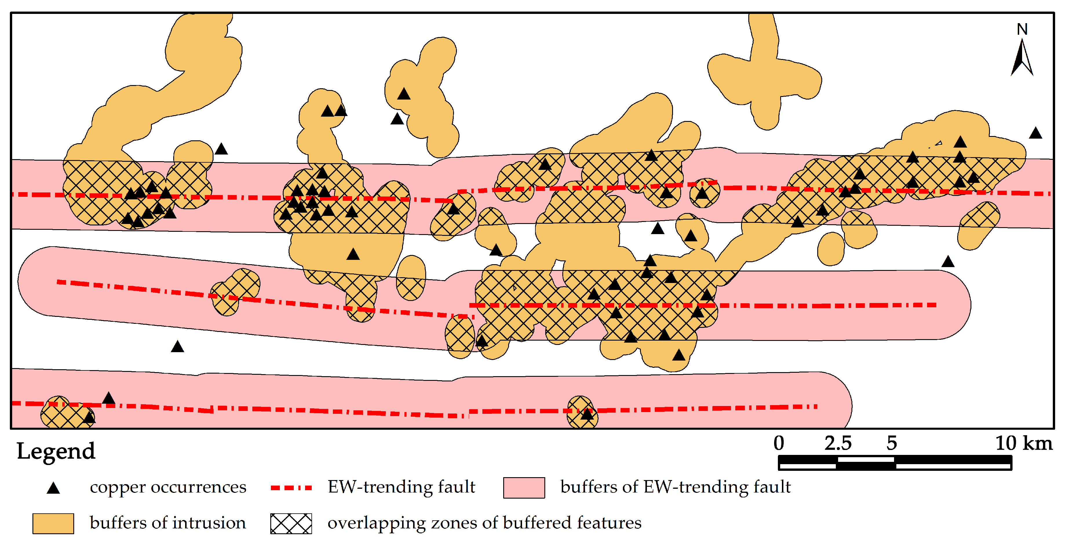
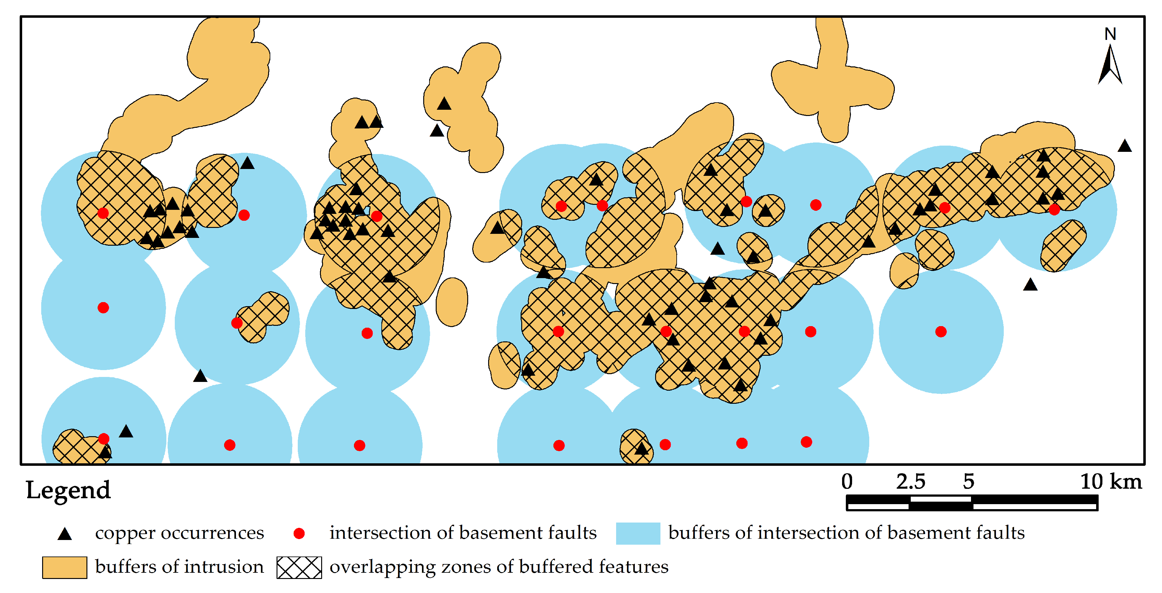
It is noteworthy that the EW-trending faults and intersections of basement faults, which show the strongest correlations with intrusions, also exhibit significant associations with copper occurrences in the previous distance distribution analysis. It is necessary to evaluate what extent of these structural controls on intrusion determine their strong correlations with copper mineralization. The EW-trending faults and Yanshanian intrusions were buffered with their optimal distances, and the copper occurrences located within the corresponding buffered zones were counted. It appears that 98% (47 out of 48) of the copper occurrences distributed within the buffers of EW-trending faults are located in the overlapping zones of the buffered EW-trending faults and intrusions which account for 33.58% of total area. Only one occurrence is included in the buffered zones where intrusions are absent (occupying 66.42% of total area) (Figure 16). Likewise, 96% (49 out of 51) of copper occurrences located within the buffers of intersections of basement faults are included in the overlapping zones of buffered intersections of faults and intrusions that occupy 37.11% of total area (Figure 17). It is inferred that the significantly strong associations of EW-trending faults and intersections of basement faults with copper mineralization are attributed to the controls of these structural features on intrusions.
3.4. Interpretation of Structural Controls on Copper Mineralization
The tectonic evolution of the TOD can be divided into four stages. The first stage is the formation and development of the basement of the Lower Yangtze Terrain (LYT) before Jinning movement (ca. 850–800 Ma) when the TOD was still an integral part of the LYT [38]. Secondly, after Jinning movement and before Indosinian movement (ca. 195 Ma), the LYT gradually developed into an archipelagic ocean stage, and the major sedimentary cover in this region formed. Contemporarily, the Cathaysian block and LYT drifted gradually to the North China Craton, leading to several soft collisions [60]. The vertical movement induced by the opening-closing effect related to soft collision was dominated in this stage, resulting in some disconformities (Table 1). Thirdly, the convergence of the Yangtze craton and North China craton (referred to as the Indosinian orogeny) commenced at the end of Triassic, which induced the formation of a series of significant structural features including angular unconformity between the Triassic and Jurassic strata (Table 1), folds and faults [35,60]. It is considered that the Indosinian movement has produced the present structural framework in the TOD, and even in the South China [39]. Eventually, the TOD experienced Yanshanian movement (ca. 135 Ma) characterized by transformation from contraction to extension since early Cretaceous [35], which induced the formation of widespread intermediate-felsic intrusions and associated mineralization. The multi-stage tectonic evolution is responsible for the structural features in both basement and sedimentary cover that are related to epigenetic copper mineralization.
The basement structures are dominated by EW- and NS-trending faults. These faults, totally overlain by Mesozoic strata, are considered to be formed before Indosinian period and reactivated in the Mesozoic [45], although the detailed geometrical and kinematical characteristics of these faults are still not clear. In previous studies, faults have been proven to act as favorable pathways for transporting ore-related magma and ore-forming fluids from deep sources to shallow trap zones, resulting in a strong association of these faults with hydrothermal mineral deposits [10,16,19]. In the study area, the petrological data and geophysical profiles evidence that a magma chamber was developed in the Mesozoic at about −10 km from the surface [42]. The EW-trending basement faults are interpreted to play a vital role of channeling the magma from the magma chamber to the shallow trap zones during the Yanshanian period. This significant control of the EW-trending faults on Yanshanian intrusions is supported by distance distribution and WofE analyses, which is fully responsible for the strong correlation between the EW-trending faults and copper mineralization. This interpretation can explain the result of Fry analysis that exhibits a predominant EW trend at regional scale.
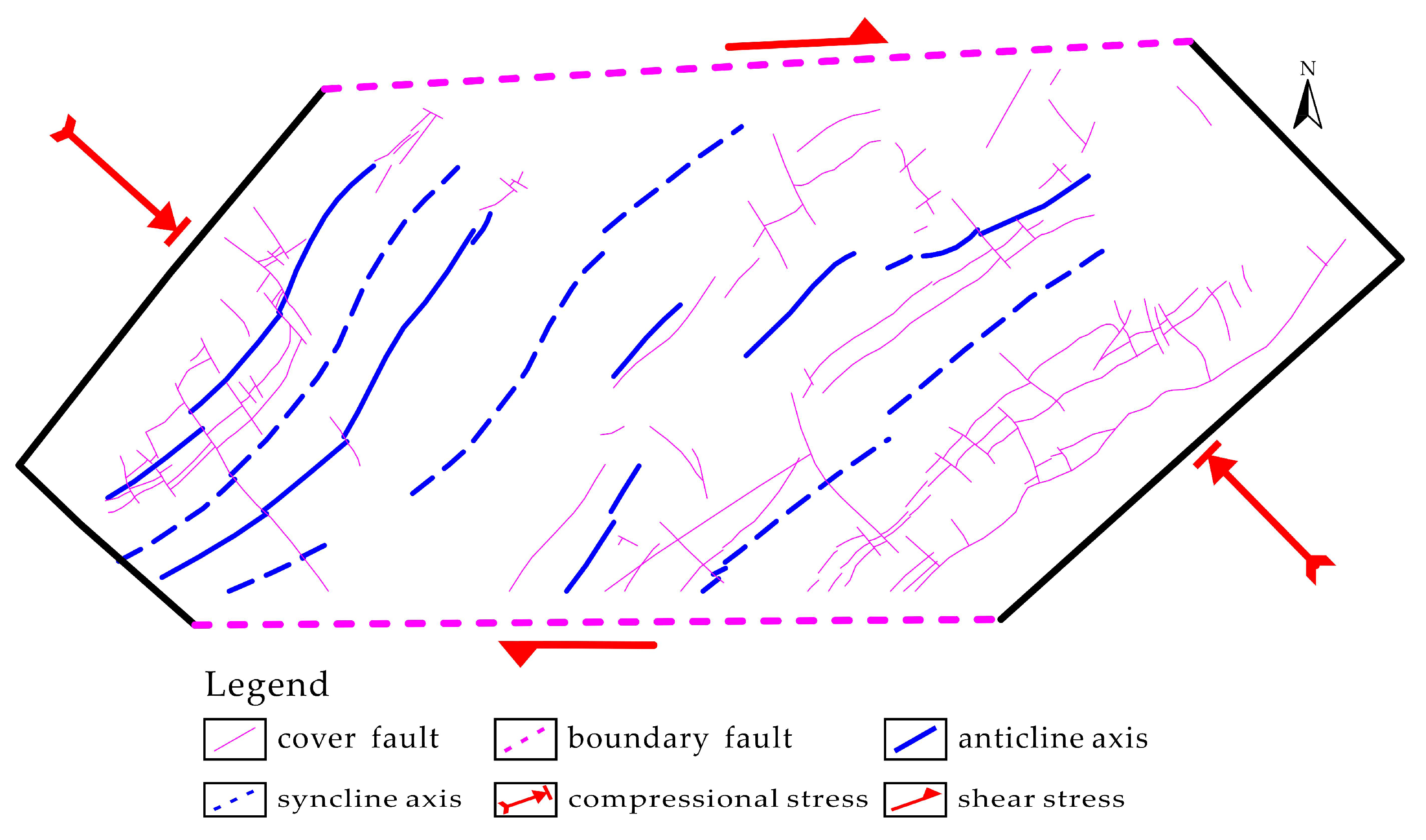
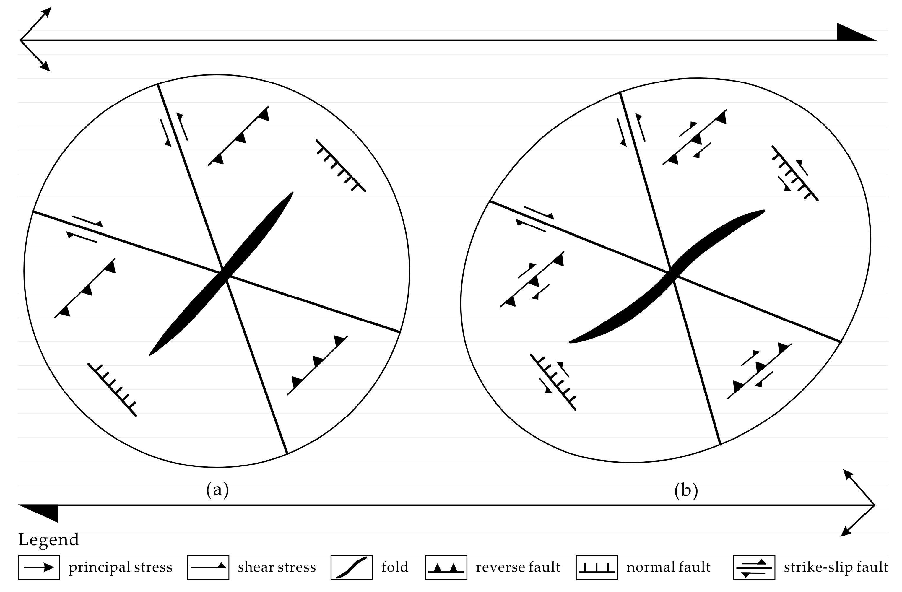
The known copper deposits are situated in the sedimentary cover where the folds with sigmoidal-shaped axes are the dominant structures, thus delineating the formative process of the folds is crucial for understanding the structural framework and copper mineralization in the cover level. Since the youngest stratum involved in the folds is Middle Triassic, it is deduced that the folds were formed during the Indosinian movement which resulted in the angular unconformity between Middle Triassic and Lower Jurassic (Table 1). A classic model of dextral simple-shear deformation in a strike-slip fault zone is introduced to illustrate the formation of folds and faults under the deformation regime of Indosinian movement dominated by NW-SE compression and dextral shear (Figure 18 and Figure 19). As the fault zone initiates, a structural system forms consisting of (i) conjugate strike-slip faults, (ii) folds, (iii) reverse faults, and (iv) normal faults (Figure 19a) [61,62]. The initially formed folds and reverse faults trend perpendicular to the direction of the greatest shortening, while the normal faults trend parallel to the direction of the greatest shortening. Subsequently, the continued strike-slip shearing can lead to a rotation of the elements in this system [62]. The axes of previously formed folds turn to sigmoidal shape. The earlier formed normal faults accommodate sinistral strike-slip motion, and the reverse faults accommodate dextral strike-slip motion (Figure 19b). The NE-trending thrust faults observed in the field [63] and sinistral strike-slip motion of NW-trending faults identified in the geological map (Figure 1) support the rationality of this model.
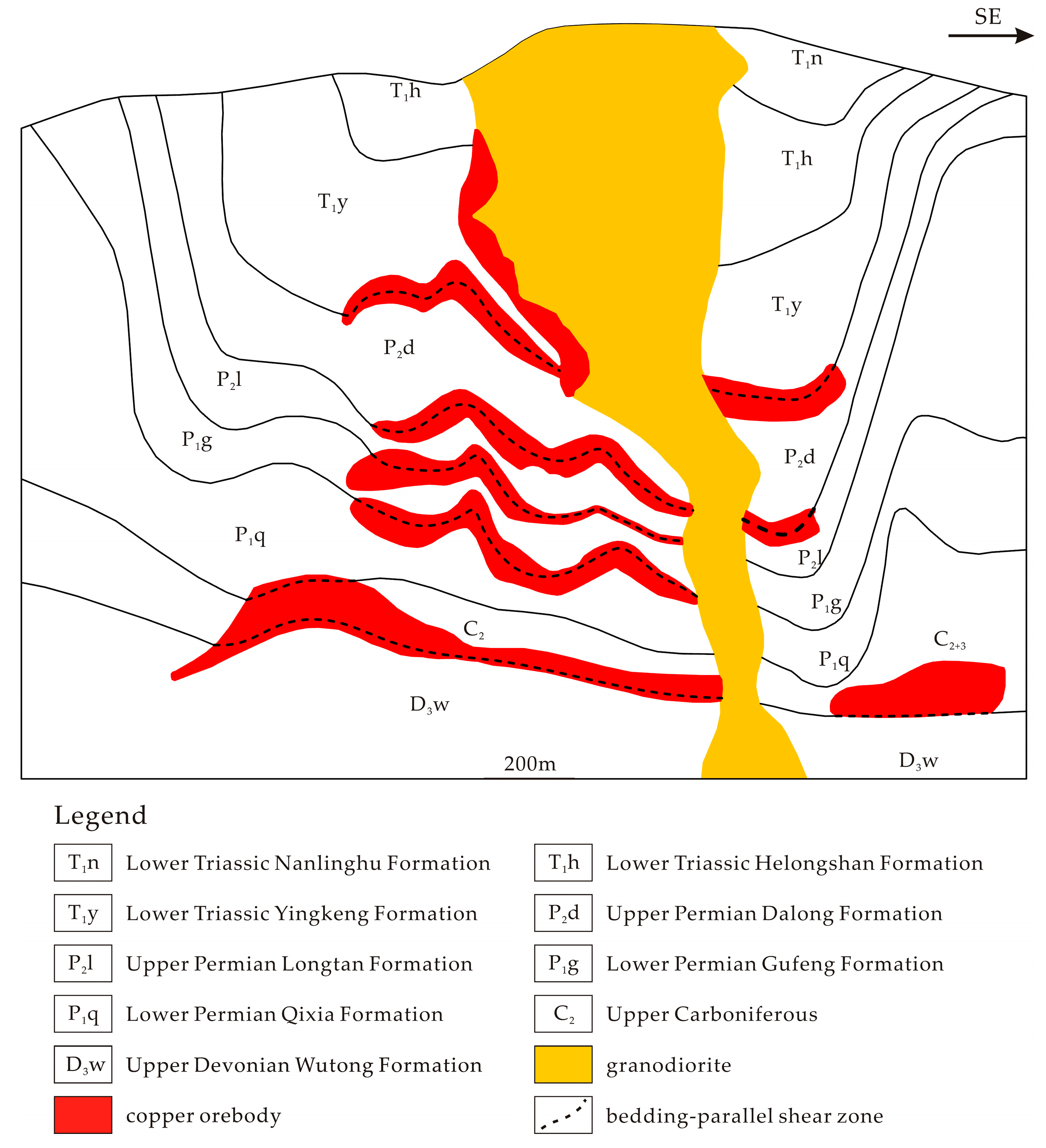
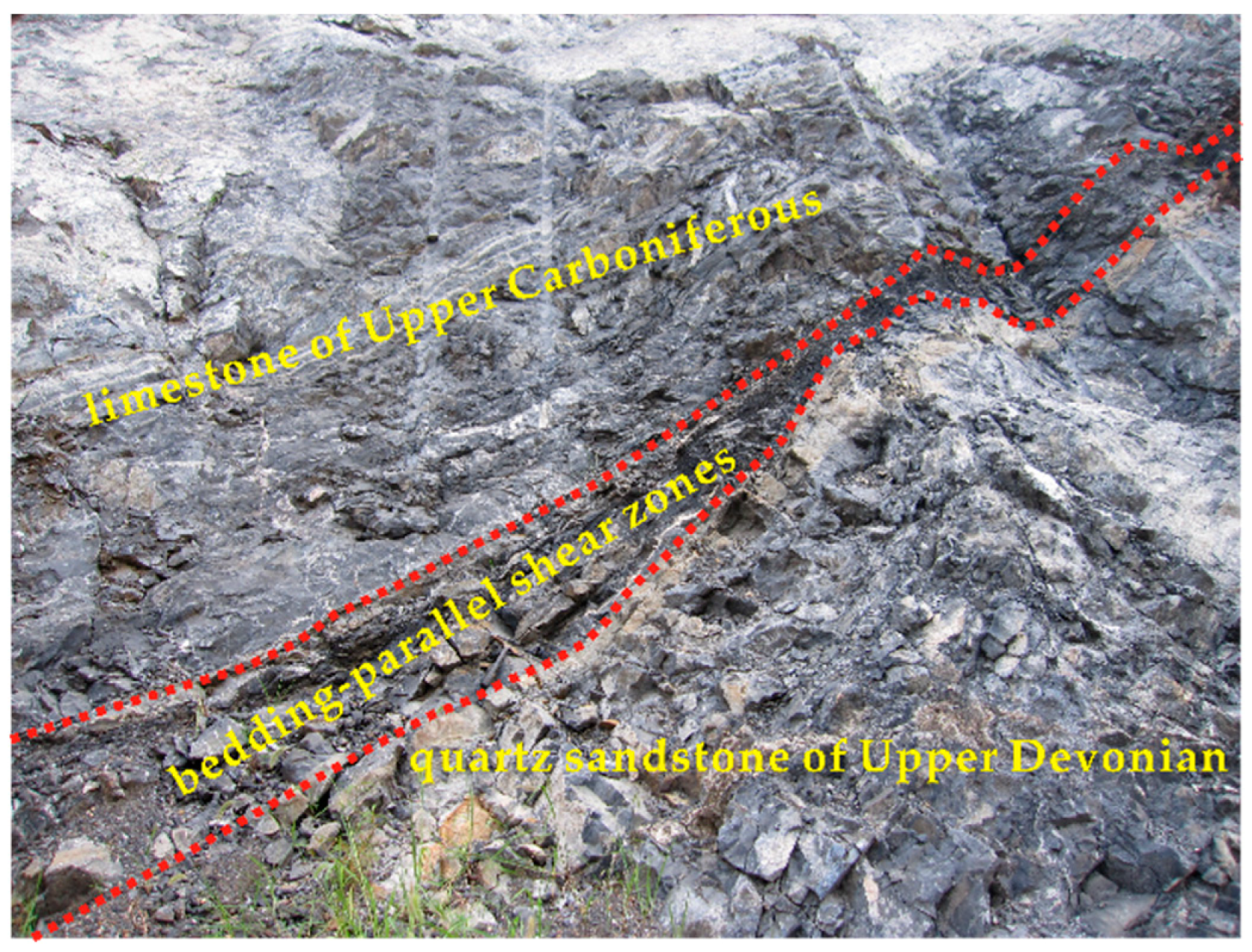
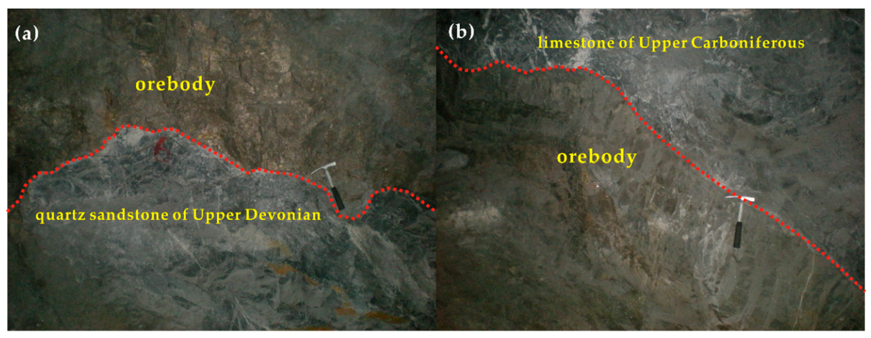
In the Mesozoic strata, there existed several interfaces between two adjacent strata which have distinct mechanical properties, some of which also represented the interfaces of disconformity, e.g., the interface between the quartz sandstone of Upper Devonian and limestone of Upper Carboniferous. During the formative process of the folds in Indosinian period, the abovementioned interfaces were subjected to the progressive deformation of folding and shearing, leading to extensive bedding-parallel shear zones [43] (Figure 20 and Figure 21). In particular, the bedding detachments occur in the cores of the folds due to the layer-parallel slippage in the formative process of folds. These shear zones were overprinted by tensional deformation in the Cretaceous when the tectonic regime in this region changed from compression to extension, thus being favorable for trapping and localizing mineralized fluids. This inference is supported by (i) the clearly discordant boundaries between stratiform orebodies and wall rocks which suggest that the ores were deposited in mechanical dilation spaces (Figure 22) [27,35,64], and (ii) the result of a numerical modeling on the Dongguashan deposit which demonstrates that the stratiform high dilation zones induced by extensional stress are favorable for fluids focusing and consistent with those positions where orebodies actually occur [64]. In addition, the bedding-parallel trap zones are located near the contacts of intrusions where sufficient sources of heat and fluid are available, and hosted in a set of carbonate strata suitable for forming skarn (Figure 20). Therefore, the bedding-parallel structures in the folded strata are favorable for hosting, focusing and depositing ore-bearing fluids, assisting in the formation of the stratabound orebodies in this area. The thickening of orebodies in the cores of folds is attributed to the detachments occurring there (e.g., major orebody within C2 in Figure 20). This interpretation is supported by distance distribution and WofE analyses, which both exhibit strong spatial association of the folds with copper mineralization. It is also inferred that the dominance of NE, NNE and NEE trends in the rose diagrams of Fry points at fine scales (<4.5 km) is attributed to the control of the folds with NE-striking axes, rather than those of the NE-trending faults which show poor correlation with copper mineralization through spatial analyses. Moreover, neither cover faults of various orientations nor the intersections of these faults show statistically significant correlation with copper mineralization, suggesting that they may only play a role in migrating the ore-bearing fluids towards the favorable host structures (i.e., multi-layered bedding-parallel shear zones) where fluid concentration and mineral deposition actually occurred, therefore leading to a lesser significant association of these cover faults with copper occurrences.
4. Conclusions
- (i)
- Fractal dimensions obtained from box-counting and radial-density analyses suggest that different structural controls operate at diverse scales of <1.5 km, 1.5–4.5 km and >4.5 km. This scale-variable controlling behavior is supported and explored by the results of Fry analysis, which illustrates a dominant EW trend at regional scale (>4.5 km) and preferential NE-NNE-NEE trends at fine scale (<4.5 km).
- (ii)
- The spatial associations of detailed structural features with copper mineralization are further investigated by quantitative spatial analyses. The Yanshanian intrusions, EW-trending faults, intersections of basement faults, and folds have significant associations with copper mineralization, indicated by their high values of quantitative parameters in both distance distribution and WofE analyses.
- (iii)
- The interpretation of structural controls on copper mineralization is made in combination of foregoing analytical results. The scale-variable patterns of mineral occurrences are attributed to the different structural controls operating in the basement and sedimentary cover. In the basement, the EW-trending faults serve as pathways for channeling magma from a magma chamber into trap zones in the caprocks during Yanshanian period. The significant control of the EW-trending faults on Yanshanian intrusion is fully responsible for the strong correlation between the EW-trending faults and copper mineralization. This inference is supported by the result of Fry analysis which shows a dominant EW trend at regional scale (>4.5 km). In the sedimentary cover, the bedding-parallel shear zones formed during Indosinian folding and shearing and overprinted by tensional deformation in Yanshanian period act as favorable sites for hosting, focusing and depositing the ore-bearing fluids, which is responsible for the dominance of NE-NNE-NEE trends at fine scale (<4.5 m) in the results of Fry analysis. Such bedding-parallel structures, together with the contact zones of intrusion, exert an important control on the formation of characteristic stratabound skarn deposits in the TOD.
Author Contributions
T.S. conducted the GIS-based computational experiments, analyzed the results and wrote the draft paper; Y.X. and X.Y. participated in the analysis of experimental results; W.L. and R.L. revised the calculation scheme; Z.H. and Y.W. collected the original data.
Acknowledgments
The research leading to this paper was jointly supported by National Natural Science Foundation of China (Grant No. 41602335), Natural Science Foundation of Jiangxi Province (Grant No. 20161BAB213084), Science and Technology Project of Jiangxi Provincial Department of Education (Grants No. GJJ150625 and No. GJJ170537), Program of Qingjiang Excellent Young Talents (Grant No. JXUSTQJYX2017001) and Doctoral Scientific Research Foundation of Jiangxi University of Science and Technology (Grant No. jxxjbs15002). We would like to express our gratitude to two anonymous Minerals reviewers for their constructive comments and suggestions that greatly improved the manuscript. Thanks are also given to Zhongfa Liu from Central South University for assistance with field evidences.
Conflicts of Interest
The authors declare no conflict of interest.
References
- Sillitoe, R.H. A plate tectonic model for the origin of porphyry copper deposits. Econ. Geol. 1972, 67, 184–197. [Google Scholar] [CrossRef]
- Tosdal, R.M.; Richards, J.P. Magmatic and structural controls on the developments of porphyry Cu ± Mo ± Au deposits. Rev. Econ. Geol. 2001, 14, 157–181. [Google Scholar]
- Kwelwa, S.D.; Dirks, P.H.G.M.; Sanislav, I.V.; Blenkinsop, T.; Kolling, S.L. Archaean gold mineralization in an extensional setting: The structural history of the Kukuluma and Matandani Deposits, Geita Greenstone Belt, Tanzania. Minerals 2018, 8, 171. [Google Scholar] [CrossRef]
- Cox, S.F.; Knackstedt, M.A.; Braun, J. Principles of structural control on permeability and fluid flow in hydrothermal systems. Rev. Econ. Geol. 2001, 14, 1–24. [Google Scholar]
- Austin, J.R.; Blenkinsop, T.G. Local to regional scale structural controls on mineralisation and the importance of a major lineament in the eastern Mount Isa Inlier, Australia: Review and analysis with autocorrelation and weights of evidence. Ore Geol. Rev. 2009, 35, 298–316. [Google Scholar] [CrossRef]
- Sillito, R.H. Iron oxide-copper-gold deposits: An Andean view. Miner. Deposita 2003, 38, 787–812. [Google Scholar] [CrossRef]
- Zeng, M.; Zhang, D.; Zhang, Z.; Liu, T.; Li, C.; Wei, C. Structural controls on the Lala iron-copper deposit of the Kangdian metallogenic province, Southwestern China: Tectonic and metallogenic implications. Ore Geol. Rev. 2018, 97, 35–54. [Google Scholar] [CrossRef]
- Chauvet, A.; Piantone, P.; Barbanson, L.; Nehlig, P.; Pedroletti, I. Gold deposit formation during collapse tectonics: Structural, mineralogical, geochronological, and fluid inclusion constraints in the Ouro Preto Gold Mines, Quadrilátero Ferrífero, Brazil. Econ. Geol. 2001, 96, 25–48. [Google Scholar] [CrossRef]
- Bonham-Carter, G.F. Geographic Information System for Geoscientists, Modeling with GIS; Pergamon: Elmsford, NY, USA, 1994; pp. 238–333. [Google Scholar]
- Haddad-Martim, P.M.; Filho, C.R.D.S.; Carranza, E.J.M. Spatial analysis of mineral deposit distribution: A review of methods and implications for structural controls on iron oxide-copper-gold mineralization in Carajás, Brazil. Ore Geol. Rev. 2017, 81, 230–244. [Google Scholar] [CrossRef]
- Schetselaar, E.; Ames, D.; Grunsky, E. Integrated 3D geological modeling to gain insight in the effects of hydrothermal alteration on post-ore deformation style and strain localization in the Flin Flon Volcanogenic Massive Sulfide Ore System. Minerals 2018, 8, 3. [Google Scholar] [CrossRef]
- Sun, T.; Wu, K.X.; Chen, L.K.; Liu, W.M.; Wang, Y.; Zhang, C.S. Joint application of fractal analysis and weights-of-evidence method for revealing the geological controls on regional-scale tungsten mineralization in Southern Jiangxi Province, China. Minerals 2017, 7, 243. [Google Scholar] [CrossRef]
- Li, X.H.; Yuan, F.; Zhang, M.M.; Jia, C.; Jowitt, S.M.; Ord, A.; Zheng, T.K.; Hu, X.Y.; Li, Y. Three-dimensional mineral prospectivity modeling for targeting of concealed mineralization within the Zhonggu iron orefield, Ningwu Basin, China. Ore Geol. Rev. 2015, 71, 633–654. [Google Scholar] [CrossRef]
- Xie, J.Y.; Wang, G.W.; Sha, Y.Z.; Liu, J.J.; Wen, B.T.; Nie, M.; Zhang, S. GIS prospectivity mapping and 3D modeling validation for potential uranium deposit targets in Shangnan district, China. J. Afr. Earth Sci. 2017, 128, 161–175. [Google Scholar] [CrossRef]
- Carranza, E.J.M. Developments in GIS-based mineral prospectivity mapping: An overview. In Proceedings of the Mineral Prospectivity, Current Approaches and Future Innovations, Orléans, France, 24–26 October 2017. [Google Scholar]
- Parsa, M.; Maghsoudi, A.; Yousefi, M. Spatial analyses of exploration evidence data to model skarn-type copper prospectivity in the Varzaghan district, NW Iran. Ore Geol. Rev. 2018, 92, 97–112. [Google Scholar] [CrossRef]
- Mandelbrot, B.B. Fractals: Form, Chances and Dimension; W.H. Freeman: New York, NY, USA, 1977; pp. 1–23. [Google Scholar]
- Roberts, S.; Sanderson, D.J.; Gumiel, P. Fractal analysis of Sn-W mineralization from central Iberia; insights into the role of fracture connectivity in the formation of an ore deposit. Econ. Geol. 1998, 93, 360–365. [Google Scholar] [CrossRef]
- Carranza, E.J.M.; Owusu, E.A.; Hale, M. Mapping of prospectivity and estimation of number of undiscovered prospects for lode gold, Southwestern Ashanti Belt, Ghana. Miner. Deposita. 2009, 44, 915–938. [Google Scholar] [CrossRef]
- Mehrabi, B.; Ghasemi, S.M.; Tale, F.E. Structural control on epithermal mineralization in the Troud-Chah Shirin belt using point pattern and Fry analyses, North of Iran. Geotectonics 2015, 49, 320–331. [Google Scholar] [CrossRef]
- Agterberg, F.P.; Bonham-Carter, G.F.; Wrigh, D.F. Statistical pattern integration for mineral exploration. In Computer Application in Resource Estimation Prediction and Assessment for Metals and Petroleum; Gaal, G., Merriam, D.F., Eds.; Pergamon: Elmsford, NY, USA, 1990; pp. 1–21. [Google Scholar]
- Cheng, Q.M.; Agterberg, F.P. Fuzzy weights of evidence method and its application in mineral potential mapping. Nat. Resour. Res. 1999, 8, 27–35. [Google Scholar] [CrossRef]
- Yuan, F.; Li, X.H.; Zhang, M.M.; Jowitt, S.M.; Jia, C.; Zheng, T.K.; Zhou, T.F. Three-dimensional weights of evidence-based prospectivity modeling: A case study of the Baixiangshan mining area, Ningwu Basin, Middle and Lower Yangtze Metallogenic Belt, China. J. Geochem. Explor. 2014, 145, 82–97. [Google Scholar] [CrossRef]
- Carranza, E.J.M. Controls on mineral deposit occurrence inferred from analysis of their spatial pattern and spatial association with geological features. Ore Geol. Rev. 2009, 35, 383–400. [Google Scholar] [CrossRef]
- Cao, Y.; Zheng, Z.; Du, Y.; Gao, F.; Qin, X.; Yang, H.; Lu, Y.; Du, Y. Ore geology and fluid inclusions of the Hucunnan deposit, Tongling, Eastern China: Implications for the separation of copper and molybdenum in skarn deposits. Ore Geol. Rev. 2017, 81, 925–939. [Google Scholar] [CrossRef]
- Liu, L.M.; Zhao, Y.L.; Zhao, C.B. Coupled geodynamics in the formation of Cu skarn deposits in the Tongling–Anqing district, China: Computational modeling and implications for exploration. J. Geochem. Explor. 2010, 106, 146–155. [Google Scholar] [CrossRef]
- Zhang, Y.; Shao, Y.J.; Li, H.B.; Liu, Z.F. Genesis of the Xinqiao Cu–S–Fe–Au deposit in the Middle-Lower Yangtze River Valley metallogenic belt, Eastern China: Constraints from U–Pb–Hf, Rb–Sr, S, and Pb isotopes. Ore Geol. Rev. 2017, 86, 100–116. [Google Scholar] [CrossRef]
- Fu, S.G.; Yan, X.Y.; Yuan, C.X. Geologic feature of submarine volcanic eruption-sedimentary pyrite type deposit in Carboniferous in the Middle-Lower Yangtze River Valley metallogenic belt, Eastern China. J. Nanjing Univ. Nat. Sci. Ed. 1977, 4, 43–67. (In Chinese) [Google Scholar]
- Gu, L.X.; Xu, K.Q. On the carboniferous submarine massive sulfide deposit in the lower reaches of the Yangtze River. Acta Geol. Sin. 1986, 60, 176–188. (In Chinese) [Google Scholar]
- Gu, L.X.; Hu, W.X.; He, J.X. Regional variations in ore composition and fluid features of massive sulfide deposits in South China: Implications for genetic modeling. Episodes 2000, 23, 110–118. [Google Scholar]
- Yang, D.F.; Fu, D.X.; Wu, N.X. Genesis of pyrite type copper in Xinqiao and its neighboring region according to ore composition and structure. Issue Nanjing Inst. Geol. Miner. Resour. Chin. Acad. Geol. Sci. 1982, 3, 59–68. (In Chinese) [Google Scholar]
- Xie, H.G.; Wang, W.B.; Li, W.D. The genesis and metallogenetic of Xinqiao Cu–S–Fe deposit, Anhui Province. Volcanol. Miner. Resour. 1995, 16, 101–107. (In Chinese) [Google Scholar]
- Zhou, T.F.; Zhang, L.J.; Yuan, F.; Fang, Y.; Cooke, D.R. LA-ICP-MS in situ trace element analysis of pyrite from the Xinqiao Cu–Au–S Deposit in Tongling, Anhui, and its constrains on the ore genesis. Earth Sci. Front. 2010, 17, 306–319. (In Chinese) [Google Scholar]
- Chang, Y.F.; Liu, X.G. Layer control type skarn type deposit—Some deposits in the Middle-Lower Yangtze Depression in Anhui Province as an example. Miner. Depos. 1983, 2, 11–20. (In Chinese) [Google Scholar]
- Pan, Y.; Dong, P. The lower Changjiang (Yangtzi/Yangtze River) metallogenic belt, East-center China: Intrusion and wall rock hosted Cu–Fe–Au, Mo, Zn, Pb, Ag deposits. Ore. Geol. Rev. 1999, 15, 177–242. [Google Scholar] [CrossRef]
- Mao, J.W.; Shao, Y.J.; Xie, G.Q.; Zhang, J.D.; Chen, Y.C. Mineral deposit model for porphyry-skarn polymetallic copper deposits in Tongling ore dense district of Middle-Lower Yangtze Valley metallogenic belt. Miner. Depos. 2009, 28, 109–119. (In Chinese) [Google Scholar]
- Zhang, Y.; Shao, Y.; Zhang, R.; Li, D.; Liu, Z.; Chen, H. Dating ore deposit using garnet U–Pb geochronology: Example from the Xinqiao Cu–S–Fe–Au deposit, Eastern China. Minerals 2018, 8, 31. [Google Scholar] [CrossRef]
- Zhou, T.; Wang, S.; Fan, Y.; Yuan, F.; Zhang, D.; White, N.C. A review of the intracontinental porphyry deposits in the Middle-Lower Yangtze River Valley metallogenic belt, Eastern China. Ore Geol. Rev. 2015, 65, 433–456. [Google Scholar] [CrossRef]
- Hu, R.Z.; Chen, W.T.; Xu, D.R.; Zhou, M.F. Reviews and new metallogenic models of mineral deposits in South China: An introduction. J. Asian Earth Sci. 2017, 137, 1–8. [Google Scholar] [CrossRef]
- Mertig, H.J.; Rubin, J.N.; Kyle, J.R. Skarn Cu–Au orebodies of the Gunung Bijih (Ertsberg) district, Irian Jaya, Indonesia. J. Geochem. Explor. 1994, 50, 179–202. [Google Scholar] [CrossRef]
- Sato, T. Manto type copper deposit in Chile—A review. Bull. Geo. Surv. Japan 1984, 35, 565–582. [Google Scholar]
- Wang, Q.F.; Deng, J.; Huang, D.H.; Xiao, C.H.; Yang, L.Q.; Wang, Y.R. Deformation model for the Tongling ore cluster region, East-Central China. Int. Geol. Rev. 2011, 53, 562–579. [Google Scholar] [CrossRef]
- Wu, G.G.; Zhang, D.; Zang, W.S. Study of tectonic layering motion and layering mineralization in the Tongling metallogenic cluster. Sci. China Ser. D Earth Sci. 2003, 46, 852–863. [Google Scholar] [CrossRef]
- Li, Y.; Li, J.W.; Li, X.H.; Selby, D.; Huang, G.H.; Chen, L.J.; Zheng, K. A carbonate replacement origin for the Xinqiao stratabound massive sulfide deposit, middle-lower Yangtze Metallogenic Belt, China. Ore Geol. Rev. 2017, 80, 985–1003. [Google Scholar] [CrossRef]
- Chang, Y.F.; Liu, X.P.; Wu, Y.C. The Copper–Iron Belt of the Low and Middle Reaches of the Changjiang River; Geological Publish House: Beijing, China, 1991; pp. 1–359. (In Chinese) [Google Scholar]
- Liu, L.M.; Yang, G.Y.; Peng, S.L.; Zhao, C.B. Numerical modeling of coupled geodynamical processes and its role in facilitating predictive ore discovery: An example from Tongling, China. Resour. Geol. 2005, 55, 21–31. [Google Scholar] [CrossRef]
- Liu, W.C.; Li, D.X.; Gao, D.Z. Analysis on the time sequence of compounding of structural deformation systems and resulting effects in Tongling area. J. Geomech. 1996, 2, 42–48. (In Chinese) [Google Scholar]
- Lü, Q.T.; Hou, Z.Q.; Zhao, J.H.; Shi, D.N.; Wu, X.Z.; Chang, Y.F.; Pei, R.F.; Huang, D.D.; Kuang, C.Y. Complex crustal structure of Tongling ore district: Insights from deep seismic reflection profiling. Sci. China Ser. D 2003, 33, 442–449. (In Chinese) [Google Scholar]
- Liu, Z.F.; Shao, Y.J.; Wei, H.T.; Wang, C. Rock-forming mechanism of Qingshanjiao intrusion in Dongguashan copper (gold) deposit, Tongling area, Anhui province, China. Trans. Nonferr. Met. Soc. China 2016, 26, 2449–2461. [Google Scholar] [CrossRef]
- Xie, J.C.; Yang, X.Y.; Sun, W.D.; Du, J.G. Early Cretaceous dioritic rocks in the Tongling region, Eastern China: Implications for the tectonic settings. Lithos 2012, 150, 49–61. [Google Scholar] [CrossRef]
- Liu, L.M.; Peng, S.L. Prediction of hidden ore bodies by synthesis of geological, geophysical and geochemical information based on dynamic model in Fenghuangshan ore field, Tongling district, China. J. Geochem. Explor. 2004, 81, 81–98. [Google Scholar] [CrossRef]
- 321 Geological Team. Structural Maps of Tongling Area; Bureau of Geological and Mineral Resources of Anhui Province: Hefei, China, 1989; pp. 1–33. [Google Scholar]
- Du, Y.L. Ore-Controlling Factors and Metallogenic Model of Stratabound Skarn Deposits in Tongling Area, Anhui Province. Ph.D. Thesis, China University of Geosciences, Beijing, China, 2013. (In Chinese). [Google Scholar]
- Zuo, R.G.; Wang, J. Fractal/multifractal modeling of geochemical data: A review. J. Geochem. Explor. 2016, 164, 33–41. [Google Scholar] [CrossRef]
- Mandelbrot, B.B. The Fractal Geometry of Nature: Updated and Augmented; W.H. Freeman: New York, NY, USA, 1983; pp. 1–31. [Google Scholar]
- Berman, M. Distance distributions associated with poisson processes of geometric figures. J. Appl. Probab. 1977, 14, 195–199. [Google Scholar] [CrossRef]
- Berman, M. Testing for spatial association between a point process and another stochastic process. J. R. Stat. Soc. C Appl. 1986, 35, 54–62. [Google Scholar] [CrossRef]
- Allek, K.; Boubaya, D.; Bouguern, A.; Hamoudi, M. Spatial association analysis between hydrocarbon fields and sedimentary residual magnetic anomalies using weights of evidence: An example from the Triassic Province of Algeria. J. Appl. Geophys. 2016, 135, 100–110. [Google Scholar] [CrossRef]
- Sang, X.J.; Xue, L.F.; Liu, J.W.; Zhan, L. A novel Workflow for geothermal prospectively mapping weights-of-evidence in Liaoning Province, Northeast China. Energies 2017, 10, 1069. [Google Scholar] [CrossRef]
- Deng, J.; Huang, D.H.; Wang, Q.F.; Hou, Z.Q.; Lü, Q.T.; Yao, L.Q.; Xin, H.B.; Zhang, Q.; Wei, Y.G. Formation mechanism of “drag depressions” and irregular boundaries in intraplate deformation. Acta Geol. Sin. 2004, 78, 267–272. [Google Scholar]
- Waldron, J.W.F. Extensional fault arrays in strike-slip and transtension. J. Struct. Geol. 2005, 27, 23–34. [Google Scholar] [CrossRef]
- David, G.H.; Reynolds, S.J.; Kluth, C.F. Structural Geology of Rocks and Regions, 3rd ed.; JohnWiley & Sons, Inc.: Westwood, MA, USA, 2011; pp. 336–338. [Google Scholar]
- Wang, Q.F. Model study of the tectonic-magmatic-metallogenical system in Tongling ore cluster area. Ph.D. Thesis, China University of Geosciences, Beijing, China, 2005. (In Chinese). [Google Scholar]
- Liu, L.M.; Sun, T.; Zhou, R.C. Epigenetic genesis and magmatic intrusion’s control on the Dongguashan stratabound Cu-Au deposit, Tongling, China: Evidence from field geology and numerical modeling. J. Geochem. Explor. 2014, 144, 97–114. [Google Scholar] [CrossRef]
Figure 1.
Geological map of the study area: (a) simplified tectonic map showing the location of the TOD; and (b) geological map of the TOD showing the locations of copper occurrences, modified from a 1:50,000 scale geological map [52] and [37,42,43,53].

Figure 2.
Schematic diagram of box-counting analysis: (a) 7 boxes containing target points with box size δ = 8; (b) 9 boxes counted with box size δ = 6; (c) 14 boxes counted with box size δ = 3; and (d) log-log plot revealing the power-law relationship of counted box number N(δ) and box size δ, obtaining box-counting fractal dimension DB = 0.7071.

Figure 3.
Schematic diagram for constructing a Fry plot: (a) the original sheet records raw points; (b) the origin O is placed on one of the raw points; (c) distribution pattern of raw points according to the origin O is transferred to the tracing sheet; (d,e) the origin O is re-placed on every raw point; (f) the tracing sheet records all distribution patterns of raw points with respect to different origins; and (g) Fry plot is constructed.

Figure 4.
Log-log plot defining the fractal dimensions of spatial pattern of copper occurrences in the TOD: (a) box-counting linear relationship; and (b) radial-density linear relationship.
Figure 4.
Log-log plot defining the fractal dimensions of spatial pattern of copper occurrences in the TOD: (a) box-counting linear relationship; and (b) radial-density linear relationship.

Figure 5.
(a) Fry plot showing spatial distribution of Fry points derived from 63 copper occurrences; and rose diagram for (b) all Fry points; (c) Fry points within 4.5 km; (d) Fry points within 1.5 km.
Figure 5.
(a) Fry plot showing spatial distribution of Fry points derived from 63 copper occurrences; and rose diagram for (b) all Fry points; (c) Fry points within 4.5 km; (d) Fry points within 1.5 km.

Figure 6.
(a) Buffer analysis and (b) graph of cumulative relative frequency concerning distance to EW-trending faults.
Figure 6.
(a) Buffer analysis and (b) graph of cumulative relative frequency concerning distance to EW-trending faults.

Figure 7.
(a) Buffer analysis and (b) graph of cumulative relative frequency concerning distance to NS-trending faults.
Figure 7.
(a) Buffer analysis and (b) graph of cumulative relative frequency concerning distance to NS-trending faults.

Figure 8.
(a) Buffer analysis and (b) graph of cumulative relative frequency concerning distance to intersections of basement faults.
Figure 8.
(a) Buffer analysis and (b) graph of cumulative relative frequency concerning distance to intersections of basement faults.

Figure 9.
(a) Buffer analysis and (b) graph of cumulative relative frequency concerning distance to folds.
Figure 9.
(a) Buffer analysis and (b) graph of cumulative relative frequency concerning distance to folds.

Figure 10.
(a) Buffer analysis and (b) graph of cumulative relative frequency concerning distance to NE-trending faults.
Figure 10.
(a) Buffer analysis and (b) graph of cumulative relative frequency concerning distance to NE-trending faults.

Figure 11.
(a) Buffer analysis and (b) graph of cumulative relative frequency concerning distance to NW-trending faults.
Figure 11.
(a) Buffer analysis and (b) graph of cumulative relative frequency concerning distance to NW-trending faults.

Figure 12.
(a) Buffer analysis and (b) graph of cumulative relative frequency concerning distance to intersections of cover faults.
Figure 12.
(a) Buffer analysis and (b) graph of cumulative relative frequency concerning distance to intersections of cover faults.

Figure 13.
Graph showing variations of higher frequencies than expected, contrasts and confidences of contrast of detailed structural features in the TOD.
Figure 13.
Graph showing variations of higher frequencies than expected, contrasts and confidences of contrast of detailed structural features in the TOD.

Figure 14.
(a) Buffer analysis and (b) graph of cumulative relative frequency concerning distance to boundaries of intrusions.
Figure 14.
(a) Buffer analysis and (b) graph of cumulative relative frequency concerning distance to boundaries of intrusions.

Figure 15.
Graph of cumulative relative frequency concerning distance to (a) EW-trending faults; (b) NS-trending faults; (c) intersections of basement faults; (d) NE-trending faults; (e) NW-trending faults and (f) intersections of cover faults.
Figure 15.
Graph of cumulative relative frequency concerning distance to (a) EW-trending faults; (b) NS-trending faults; (c) intersections of basement faults; (d) NE-trending faults; (e) NW-trending faults and (f) intersections of cover faults.


Figure 16.
Buffer analysis showing the distribution of copper occurrences in buffered EW-trending faults and intrusions.
Figure 16.
Buffer analysis showing the distribution of copper occurrences in buffered EW-trending faults and intrusions.

Figure 17.
Buffer analysis showing the distribution of copper occurrences in buffered intersections of basement faults and intrusions.
Figure 17.
Buffer analysis showing the distribution of copper occurrences in buffered intersections of basement faults and intrusions.

Figure 18.
Stress regime during the formative process of the folds with sigmoidal axes, modified from [42].
Figure 18.
Stress regime during the formative process of the folds with sigmoidal axes, modified from [42].

Figure 19.
Deformation model of dextral shearing in a strike-slip fault zone, modified from [61]. (a) a structural system formed in initial stage of deformation; and (b) a rotation of structural elements during continued strike-slip shearing.
Figure 19.
Deformation model of dextral shearing in a strike-slip fault zone, modified from [61]. (a) a structural system formed in initial stage of deformation; and (b) a rotation of structural elements during continued strike-slip shearing.

Figure 20.
Typical cross-section of Shizishan ore field showing the characteristic stratabound skarn orebodies hosted in the folds, modified from [43].
Figure 20.
Typical cross-section of Shizishan ore field showing the characteristic stratabound skarn orebodies hosted in the folds, modified from [43].

Figure 21.
Field photograph of outcropped bedding-parallel shear zone between limestone of Upper Carboniferous and quartz sandstone of Upper Devonian in the Xinqiao deposit.
Figure 21.
Field photograph of outcropped bedding-parallel shear zone between limestone of Upper Carboniferous and quartz sandstone of Upper Devonian in the Xinqiao deposit.

Figure 22.
Photographs showing the discordant boundaries between stratiform orebodies and wall rocks in the Xinqiao deposit. (a) the boundary between orebody and underlying Upper Devonian quartz sandstone; and (b) the boundary between orebody and overlying Upper Carboniferous limestone.
Figure 22.
Photographs showing the discordant boundaries between stratiform orebodies and wall rocks in the Xinqiao deposit. (a) the boundary between orebody and underlying Upper Devonian quartz sandstone; and (b) the boundary between orebody and overlying Upper Carboniferous limestone.


Table 1.
Stratigraphy and tectonic events in the Tongling ore district
| Epoch | Lithostratigraphic Unit | Code | Lithological Description | Tectonic Activity |
|---|---|---|---|---|
| Upper Cretaceous | Xuannan Formation | K2x | Conglomerate and sandstone | Yanshanian movement (ca. 135 Ma) |
| Middle Jurassic | Luoling Formation | J2l | Feldspar sandstone, siltstone and shale | |
| Lower Jurassic | Moshan Formation | J1m | Feldspar sandstone with interlays of silty shale and coal, conglomerate at bottom | Indosinian movement (ca. 195 Ma) |
| Middle Triassic | Tongtoujian Formation | T2t | Siltstone with interlays of sandy shale | |
| Yueshan Formation | T2y | Limestone, dolomite in upper and siltstone in lower | ||
| Lower Triassic | Nanlinghu Formation | T1n | Limestone | |
| Helongshan Formation | T1h | Limestone | ||
| Yingkeng Formation | T1y | Limestone with interlays of silt shale | ||
| Upper Permian | Dalong Formation | P2d | Siliceous shale with interlays of limestone | |
| Longtan Formation | P2l | Fine sandstone and silt shale with interlays of coal | ||
| Lower Permian | Gufeng Formation | P1g | Siliceous slate and siliceous shale | |
| Qixia Formation | P1q | Bioclastic limestone in upper and carbonaceous shale in lower | ||
| Upper Carboniferous | Chuanshan Formation | C2c | Orbicular limestone and bioclastic limestone | |
| Huanglong Formation | C2h | Bioclastic limestone and dolomite | ||
| Upper Devonian | Wutong Formation | D3w | Quartz sandstone and silty shale | |
| Middle Silurian | Fentou Formation | S2f | Sandstone, siltstone and sandy shale | |
| Lower Silurian | Gaojiabian Formation | S1g | Black shale | |
| Upper Ordovician | Wufeng Formation | O3w | Black siliceous shale | |
| Tangtou Formation | O3t | Calcareous shale with interlayers of limestone | ||
| Middle Ordovician | Tangshan Formation | O2t | Limestone with interlayers of thin slate | |
| Lower Ordovician | Lunshan Formation | O1l | Limestone in upper and dolomite in lower | |
| Cambrian | Huangjiabang Formation | є | Limestone | |
| Precambrian | Dongling Group | Pt3d | Biotite quartz schist and gneiss | Jinning movement (ca. 850–800 Ma) |
Modified from [26]; dashed line represents disconformity; and double line represents angular unconformity.
Table 2.
Results of distance distribution and WofE analyses.
| Structural Features | Optimal Buffer Distance (m) | Distance Distribution Analysis | WofE Analysis | ||||
|---|---|---|---|---|---|---|---|
| DM | DN | D | uc | C | Cs | ||
| EW-trending faults | 1500 | 76% | 55% | 21% | 75% | 1.36 | 4.6 |
| NS-trending faults | 1000 | 55% | 53% | 2% | 72% | 0.2 | 0.8 |
| intersections of basement faults | 2500 | 83% | 60% | 23% | 79% | 1.54 | 4.64 |
| folds | 2500 | 89% | 67% | 22% | 86% | 1.59 | 3.95 |
| NE-trending faults | 1500 | 68% | 57% | 11% | 76% | 0.63 | 2.33 |
| NW-trending faults | 1500 | 59% | 49% | 10% | 68% | 0.44 | 1.74 |
| intersections of cover faults | 2500 | 74% | 65% | 9% | 84% | 0.71 | 2.46 |
| contact of Yanshanian intrusion | 350 | 87% | 21% | 55% | 52% | 3.04 | 8.03 |
DM: cumulative relative frequency of copper occurrence; DN: cumulative relative frequency of non-occurrence; D: DN − DN; uc: upper confidence band for the curve DN; C: contrast value; and Cs: confidence of contrast.
© 2018 by the authors. Licensee MDPI, Basel, Switzerland. This article is an open access article distributed under the terms and conditions of the Creative Commons Attribution (CC BY) license (http://creativecommons.org/licenses/by/4.0/).
Share and Cite
MDPI and ACS Style
Sun, T.; Xu, Y.; Yu, X.; Liu, W.; Li, R.; Hu, Z.; Wang, Y. Structural Controls on Copper Mineralization in the Tongling Ore District, Eastern China: Evidence from Spatial Analysis. Minerals 2018, 8, 254. https://doi.org/10.3390/min8060254
AMA Style
Sun T, Xu Y, Yu X, Liu W, Li R, Hu Z, Wang Y. Structural Controls on Copper Mineralization in the Tongling Ore District, Eastern China: Evidence from Spatial Analysis. Minerals. 2018; 8(6):254. https://doi.org/10.3390/min8060254
Chicago/Turabian StyleSun, Tao, Ying Xu, Xuhui Yu, Weiming Liu, Ruixue Li, Zijuan Hu, and Yun Wang. 2018. "Structural Controls on Copper Mineralization in the Tongling Ore District, Eastern China: Evidence from Spatial Analysis" Minerals 8, no. 6: 254. https://doi.org/10.3390/min8060254
Note that from the first issue of 2016, this journal uses article numbers instead of page numbers. See further details here.