Temporal Evolution of Calcite Surface Dissolution Kinetics

Abstract

This brief paper presents a rare dataset: a set of quantitative, topographic measurements of a dissolving calcite crystal over a relatively large and fixed field of view (~400 μm²) and long total reaction time ($>6\mathrm{h}$). Using a vertical scanning interferometer and patented fluid flow cell, surface height maps of a dissolving calcite crystal were produced by periodically and repetitively removing reactant fluid, rapidly acquiring a height dataset, and returning the sample to a wetted, reacting state. These reaction-measurement cycles were accomplished without changing the crystal surface position relative to the instrument’s optic axis, with an approximate frequency of one data acquisition per six minutes’ reaction (~10/h). In the standard fashion, computed differences in surface height over time yield a detailed velocity map of the retreating surface as a function of time. This dataset thus constitutes a near-continuous record of reaction, and can be used to both understand the relationship between changes in the overall dissolution rate of the surface and the morphology of the surface itself, particularly the relationship of (a) large, persistent features (e.g., etch pits related to screw dislocations; (b) small, short-lived features (e.g., so-called pancake pits probably related to point defects); (c) complex features that reflect organization on a large scale over a long period of time (i.e., coalescent “super” steps), to surface normal retreat and step wave formation. Although roughly similar in frequency of observation to an in situ atomic force microscopy (AFM) fluid cell, this vertical scanning interferometry (VSI) method reveals details of the interaction of surface features over a significantly larger scale, yielding insight into the role of various components in terms of their contribution to the cumulative dissolution rate as a function of space and time.

1. Introduction

The thermodynamic reactions on minerals surface determines their stability and fate in a given environment. As these reactions drive a series of natural (e.g., nutrient release and availability, soil pH buffering, carbon cycling, water acidification) and industrial processes (e.g., geological CO₂ sequestration, cement hydration, weathering, and corrosion of industrial structures), understanding their kinetics is a key focus of environmental science. Despite an ongoing debate over uncertainties in predicting long-term mineral dissolution rates in a wide spectrum of environments, there is general agreement that such predictive capabilities depend on understanding fundamental reaction mechanisms at the mineral-fluid interface, as well as their variation in time and space [1].

Prior to the advent of atomic force microscopy (AFM), vertical scanning interferometry (VSI), and related surface microscopic techniques, distinguishing potential sources of variation in dissolution rate using conventional bulk-powder experiments (data are summarized in refs. [2,3,4] was generally not feasible. The currently widespread use of these instruments has yielded a detailed understanding of the interaction of minerals with their ambient solution (e.g., ref. [5]). Both microscopes afford direct observation of mineral surfaces, and in situ AFM [6,7,8,9,10,11,12] and VSI [1,13,14,15,16,17] have greatly expanded the understanding of reaction kinetics for a diverse range of carbonates, silicates, and other important phases. Calcite has been a favorite AFM and VSI target, due to its clear importance in environmental systems, its simple composition, and perfect cleavage. For example, early in situ AFM work determined the crystallographic control of the velocity of atomic scale steps in pure solutions [18], documenting the anisotropic specificity of kink and step orientations. These site-specific properties reflect in part the oblique intersection of the hexagonal unit cell with the ($10\overline{1}4$) cleavage surface. This obliquity generates unique kink sites and step edges (i.e., the $\langle \overline{4}41\rangle ,\langle 48\overline{1}\rangle$ step directions are crystallographically equivalent, but opposite-facing step pairs are not), and specific geometries in calcium-oxygen coordination give rise to corresponding orientation-specific properties. In the study of calcite dissolution kinetics, a major AFM research focus has been the relationship of step velocity, spacing, geometry, and related observables to solution properties (pH, dissolved lattice ions, impurity components, supporting electrolytes, ionic strength, etc.; see citations above). This detailed work, spanning the early 1990′s to the present day, has yielded a rich set of observations and measurements, now augmented with significant thermodynamics modeling and kinetics simulation [19,20,21,22]. As a result, calcite is one of the best-studied crystals of environmental significance in terms of the relationship between its dissolution rate and the physics and chemical structure of its surface. However, despite the overall simplicity of calcite’s structure, these datasets have also revealed significant complexity in step movement and morphology. This complexity implies that the general morphology of the surface is a sensitive reflector, not only of its interactions with the surrounding solution, but with itself as well (see e.g., ref. [23]). Variations in morphology are tied to heterogeneities in rate, phenomena we have termed intrinsic variations (tied to crystallographic and microstructural factors), to distinguish them from those arising from environmental inputs of purely extrinsic origin [24]. As rate controls, the latter environmental factors are no less important, and significant effort has been devoted to understanding their influence [25]. Here, however, we wish to focus entirely on intrinsic variation in rate expressed over the calcite surface.

As mentioned above, detailed AFM studies of dissolving calcite have made critical advances in quantifying the dynamics of surface features at or close to the atomic scale [26,27], and have focused largely on step movement. The AFM studies conducted in situ have easily detailed the anisotropy in step velocities, quantifying the variation of crystallographically inequivalent “obtuse”$\left({\left[\overline{4}41\right]}_{+},{\left[48\overline{1}\right]}_{+}\right)$ and “acute” $\left({\left[\overline{4}41\right]}_{-},{\left[48\overline{1}\right]}_{-}\right)$ steps as a function of saturation state, impurity burden, pH, ionic strength, and other controls (work reviewed in ref. [11]). From these data, the overall rate of dissolution has often been quantified by essentially integrating step velocity over time, e.g., $v_{\perp }=v_s\left(h_s/\mathsf{\Lambda }\right)$, where the surface normal retreat velocity ($v_{\perp }$) is computed from the step velocity ($v_s$), step height ($h_s$), and the standard terrace width ($\mathsf{\Lambda }$) separating a step from its neighbor; the rate in units of moles per unit area per unit time can then be given as $r=v_{\perp }/\overline{V}$, where $\overline{V}$ is the molar volume. Alternatively, the mean rate over an AFM field of view can be computed as $r={\overline{V}}^{-1}{\overline{v}}_s\overline{\left(\frac{\partial z}{\partial x}\right)}$, where $\overline{\left(\frac{\partial z}{\partial x}\right)}$ is the mean surface gradient, and ${\overline{v}}_s$ is the mean step velocity. More elaborate means of achieving surface normal retreat rates may also involve quantification of the volume and number of etch pits (also reviewed in ref. [11]), but these methods may ignore the background layer-by-layer removal of material (the “global” rate [15]), as well as the inherent coupling between etch pits associated with deep screw dislocations and the surface normal deflation rate, conceptually formalized in the step wave model [28]. We have made this point before, i.e., that while AFM’s in situ capabilities provide exquisite and invaluable detail of the dynamics of surface features in minerals over small areas of interest, cantilever constraints do limit the depth—and thus the area—that can be effectively measured. This limit makes the study of variation in dissolution rates problematic, as it is easy to imagine how local step velocities and spacing may be influenced by events or features outside the AFM’s immediate field of view. VSI, with a significantly larger field of view, supplies rapid and robust acquisition of surface height data at high vertical resolution, and height changes are absolute over time when acquisition of data is made in conjunction with a masked or coated reference surface. In terms of measurement of dissolution rates, VSI’s limitations are its lateral resolution—a function of the objective’s numerical aperture (see ref. [4], for discussion), and the complexity of direct, truly in situ measurements, which must be compensated for the fluid’s contribution to the optic signal (see also in situ digital holographic microscopy in ref. [17]). These limits are often the motivation for using AFM and VSI instruments in concert as complementary tools.

Here, as a means of approaching the basic problem of spatial and temporal rate variation raised in earlier papers [1,15,24], we wish to explore what can be learned from continuous observation of a single crystal in a simple solution for an extended period. Using an open fluid cell and large calcite single crystal, we developed a so-called near in-situ VSI cell, in which a fluid of fixed composition flows rapidly over the surface, a surface that is fixed relative to the instrument’s optic path. During reaction, all relevant environmental conditions (flow rate, temperature, pH) are also held constant. Periodically, fluid is rapidly removed from the surface for a period sufficient for data acquisition, after which flow is restored. The sample is again allowed to react, and the sequence repeated. In this manner, a high number of near-continuous measurements (80) were acquired over a large (414 × 313 µm², ~0.13 mm²), fixed region of the surface for 6 h reaction time. In many AFM and VSI experiments, a common protocol is to cleave the sample prior to solution contact, thus introducing a “pristine” initial condition. In contrast, we reacted the surface for ~2 days under flow conditions prior to first measurements. In our view, the resulting observational record constitutes a unique dataset, and allows us to quantify how a statistically significant area of the surface changes over time as dissolution proceeds. We can thus begin to address a basic question: does a steady state surface exist? Can the concept of steady state dissolution, underpinning much of our understanding and experimental approach, be reasonably defended? Does a steady state surface have a statistical signature? These questions constitute our basic motivations.

2. Methods

The reactant solution used here was identical in composition to that used in previous work [15], prepared by dissolving sufficient reagent grade Na₂CO₃ within a large volume of deionized water (30 L, 18.2 MΩ-cm) to give a total alkalinity of 4.4 meq/kg-H₂O. After preparation, this solution was sparged with water-saturated laboratory air to attain equilibrium with respect to atmospheric pCO₂ and a stable pH (8.82 at 22 °C, measured by Orion semimicro combination glass electrode). Constant sparging was sufficient to agitate the solution over the course of the experiment and produced a pH stable over 25 h (within ±0.02 pH units). This solution contained essentially no calcium and was thus highly under-saturated with respect to calcite. Input solution temperature was maintained at 22 °C. The sample crystal was prepared by gentle cleaving of a large synthetic calcite crystal with a razor to produce a $\left(10\overline{1}4\right)$ cleavage fragment, which was then affixed to the cell surface between the flow path of the input and scavenging ports (Figure 1).

Similar to much of our previous work (e.g., refs. [15,30]), we used a MicroXAM (ADE Phase Shift, now KLA-Tencor) commercial vertical scanning interferometer (KLA-Tencor Co., Milpitas, CA, USA) equipped with Nikon Mirau objectives (10×, 20×, 50×, and 100× magnification), white light source (550 nm center wavelength), and high-resolution CCD (750 × 480 pixels). This instrument was mounted on an air-suspension table in a vibration-isolated laboratory. Details regarding the general theory of operation, acquisition and treatment of data using this instrument are available in Luttge and Arvidson [31].

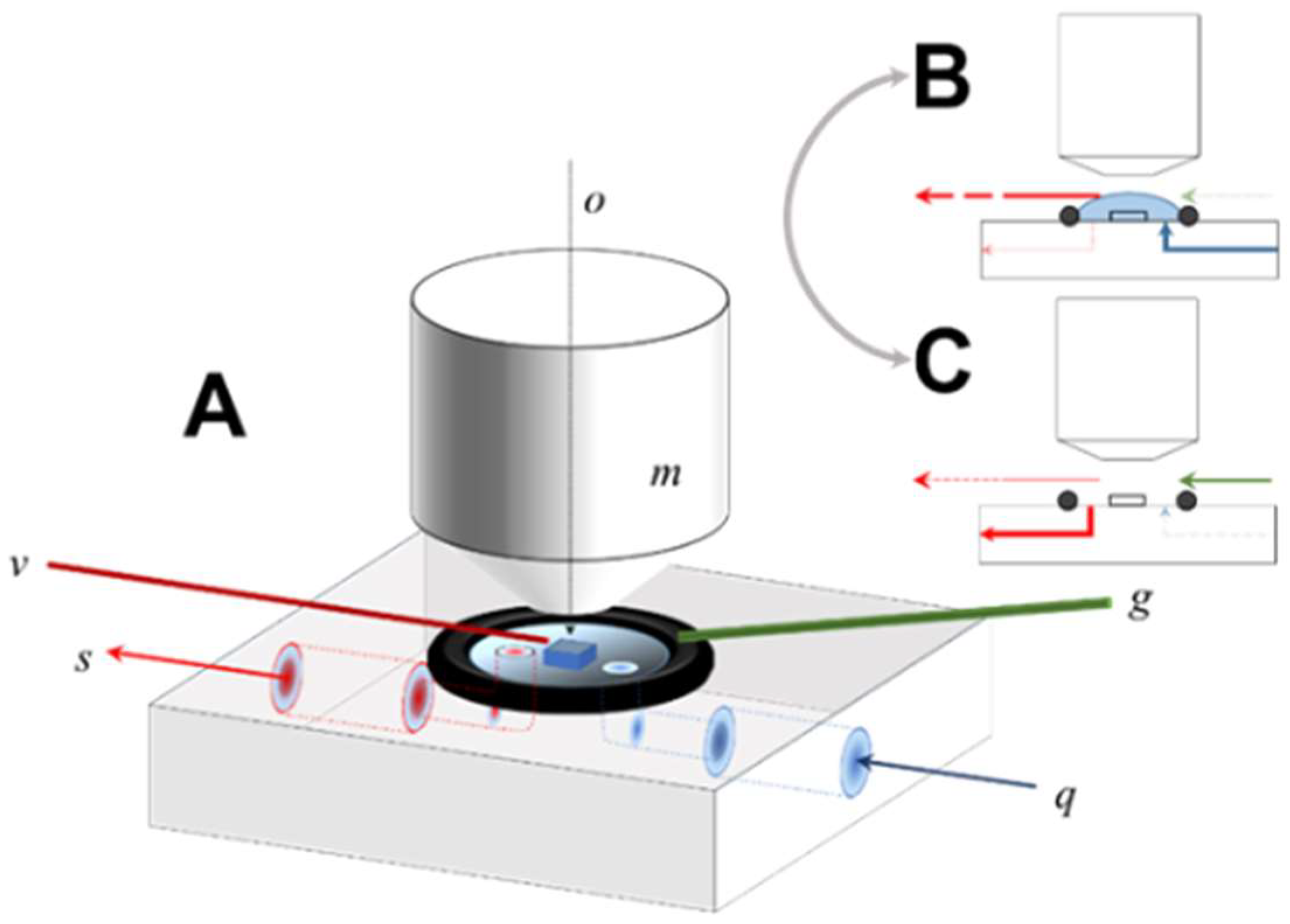
The fluid cell is extremely simple in design, fabricated from polyether ether ketone (PEEK) and consisting of internal ports for fluid input to and removal from an open reaction fluid volume [29]. Reactant fluid was delivered to the cell by a peristaltic pump at a volumetric flow rate of ~6 mL per minute, thus giving well-mixed fluid residence times of less than 8 s, sufficiently brief to eliminate transport dependency and maintain far-from-equilibrium conditions based on comparison with previous experiments [15]. As shown in Figure 1, fluid introduced to the cell’s open surface through the input channel (q) is confined laterally by a Viton O-ring, resulting in complete immersion of the sample crystal in the process.

During reaction mode (Figure 1B), the fluid parcel is maintained and continuously withdrawn by a capillary vacuum aspirator suspended a few mms over the sample surface. The total fluid volume is thus to some extent variable (although typically <0.5 mL), a function of the balance between the input flow pump rate versus the position and pressure drop of the capillary; no fluid is removed by the scavenging port during reaction. The capillary position is micro-adjusted so that the crystal sample is mechanically undisturbed, preventing contact of the upper surface of the fluid with the Mirau objective, thus maintaining registration of the sample surface with respect to the optic path of the interferometer during the entire experiment. Drift of the sample position with respect to the optic path was not rigorously quantified, but is in the range of a single pixel, verified by ad hoc comparison of the pixel position of fiducial landmarks over time.

To shift to data acquisition mode (Figure 1B,C), the input flow was diverted, the scavenging port opened to a vacuum line, and fluid rapidly removed from the entire cell. The instrument’s focal condition and fringe position is then zeroed, and data acquisition completed using a 10 µm scan length. After data acquisition was complete, the cell was returned to flow operation (Figure 1B). In practice this cycle (wet-dry-wet) could be accomplished in ~20 s.

After the mounting of the sample in the cell but prior to collection of the data shown in this paper, the sample was reacted continuously at pH 8.82 for more than 48 h, thus allowing substantial dissolution of the initially prepared surface. The field of view was then fixed and focused using a 20× objective, and topographic data collected at roughly 5-min intervals for 6 h using the above control cycle, yielding 80 total datasets (field of view 414 × 313 µm²). These measurements and subsequent calculations constitute the total dataset presented in this paper. Because measurements are obtained over the same field of view, the resulting sequence can be used to evaluate the overall morphological changes in surface topography. In addition, we subtracted various height maps to a produce a corresponding difference map, showing the spatial distribution of dissolution flux. These changes were also evaluated by comparison of surface gradient maps, i.e., the surface derivative or change in slope within a single dataset. A gradient or derivative map effectively flattens the surface allowing us to highlight surface features that otherwise differed in absolute height by hundreds of nanometers up to microns. For example, with this approach we can thus reveal the distribution of shallow, pancake pits forming at point defects simultaneously with deep etch pits forming at the hollow cores of screw dislocations. Comparison of gradient maps also allowed us to detect and confirm areas of the surface over which changes in absolute height due to dissolution were minimal, and thus could effectively serve as reference areas. This was necessary as no mask was used to explicitly create a non-reactive reference area in this experiment; in practice, these flux measurements thus represent a minimum rate, as some surface retreat may have occurred between measurements. Given our purpose, this issue is of limited importance: these errors will be small because of the correspondingly small vertical z-contribution of global retreat (lateral changes in surface topography also afford a check on the spatial distribution of reactivity) and will not interfere with our focus on the spatial distribution of rates and their statistical distribution.

Potential Topography Evolution of Smooth Surface Plateau Sections

Plateau sections are considered to be unreactive in such cases that no evolution of nanotopography (>1 nm, precision of the method) has been observed using interferometry techniques.

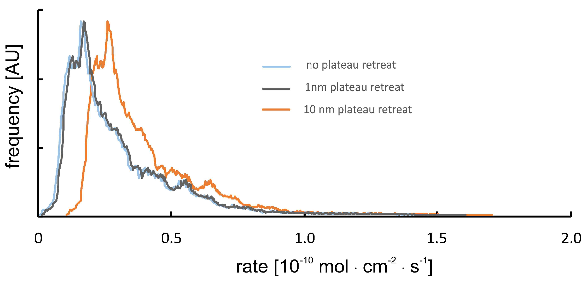
This assumption is incorrect if multiple calcite layers (i) show a high density and homogeneous distribution of point defects, and (ii) their dissolution results in a very smooth surface (roughness <1 nm) after several tens of minutes of reaction time. In such cases (not observed in our data sets), we need to correct for the position of the calculated rate spectra with respect to the absolute rate values (x-axis). Such a correction always results in an increase of the overall rate, cf. Figure 2.

The sensitivity of the instrument and the resulting uncertainty of calculated rate spectra are illustrated by the positions of the blue vs. gray rate curves. In the case of a surface normal retreat, that is one order of magnitude bigger than the sensitivity of the instrument, the rate curve would shift to the position of the orange-colored line.

The occurrence of such a situation and a resulting error as shown is, however, unlikely. Any bigger retreat of surface plateaus, that are considered to be unreactive, would result in a few surface portions of the rate maps that show surface growth. We did, however, not observe such behavior thus assuming the uncertainty of reported rate curves is rather close to the 1 nm roughness situation instead of the 10 nm retreat rate curves, as shown in Figure 2.

3. Results

3.1. Dissolution Rate Maps and Rate Spectra

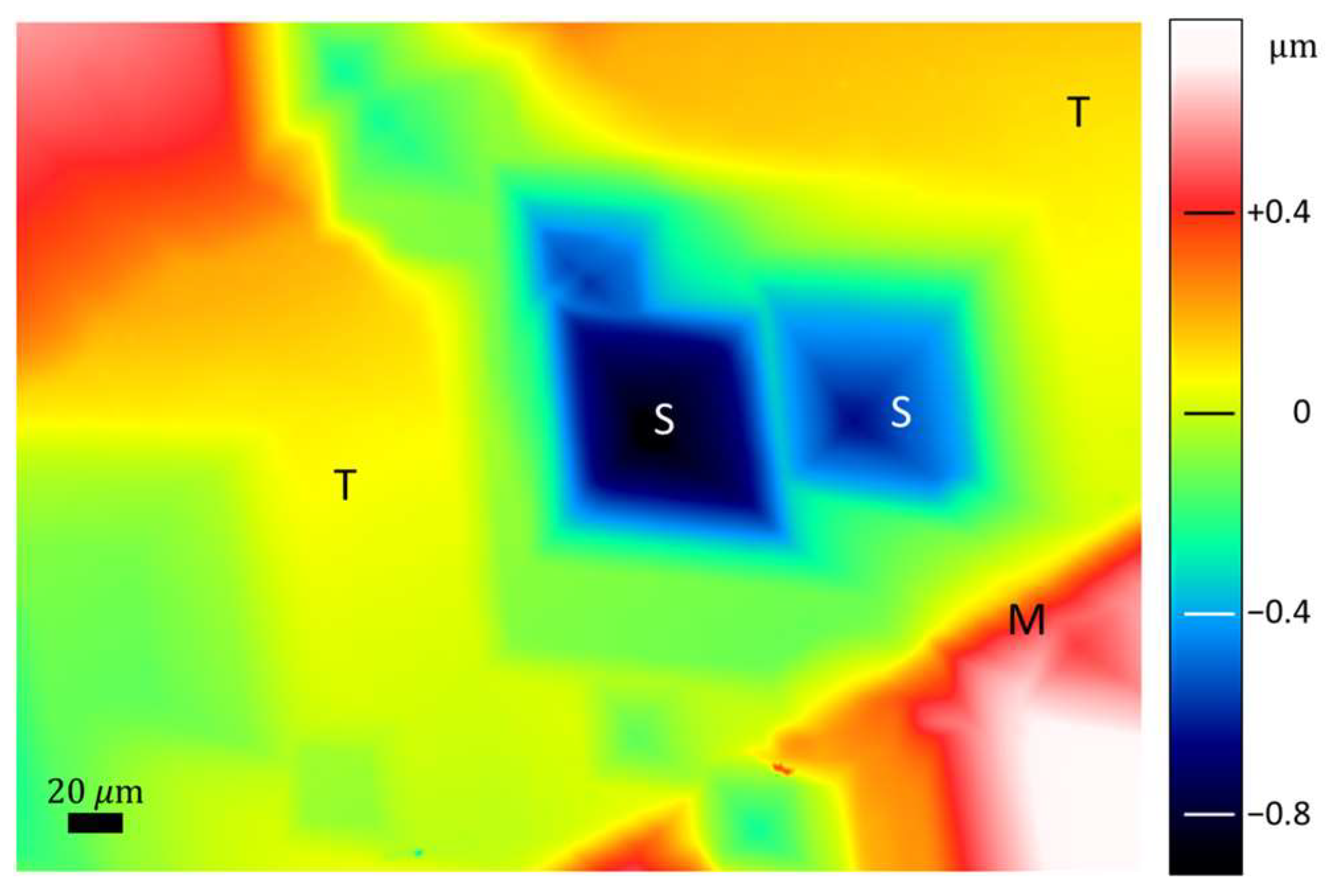
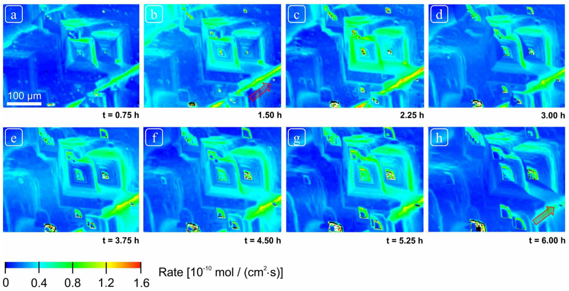
The initial height map is shown in Figure 3 (i.e., prior to the start of the sequence but after 48 h reaction), and shows several large, well-developed etch pits (the outcrop of deep screw dislocations), low relief terraces with only minor pits, and a large step-like feature (“M” in Figure 3) we shall discuss later, giving a total height range of 1.7 µm. Figure 4 shows the sequence of rate (difference) maps computed from VSI surface topography measurements at eight consecutive time steps: t = 0.75, 1.50, 2.25, 3.00, 3.75, 4.5, 5.25, and 6.00 h. The first time step, Figure 4a, thus represents the difference in height between data collected at t = 0 and t = 0.75 h, with the rate (denoted in the color map) computed by dividing these difference map by the elapsed time and molar volume; similarly, the second time step is the difference map between t = 0.75 and t = 1.50 h, and so on. These maps illustrate the large spatial variability in dissolution rate, as well as its variation over time. Differences exceeding an order of magnitude are immediately apparent, with a total range of ~ 0.1 × 10⁻¹⁰ mol·cm⁻²·s⁻¹ and 1.6 × 10⁻¹⁰ mol·cm⁻²·s⁻¹. Lower rates (≤0.3 × 10⁻¹⁰ mol·cm⁻²·s⁻¹) are distributed over large portions of the surface (terraces areas ‘T’ in Figure 3) that otherwise lack deep etch pits. Intermediate rates (between >0.3 × 10⁻¹⁰ and <0.5 × 10⁻¹⁰ mol·cm⁻²·s⁻¹) are typical of areas of surface normal retreat (upper left corner) and the steep, interior walls of large etch pits. The highest rates, ranging between ≥0.5 × 10⁻¹⁰ mol·cm⁻²·s⁻¹ and ≤0.8 × 10⁻¹⁰ mol·cm⁻²·s⁻¹, are found at the upper shoulder of large pits (i.e., at the change in slope that marks the macroscopic pit boundary with the surrounding terrace), as well as the stepped feature (“M” in Figure 3). This stepped feature is the most unusual aspect of the surface observed in the entire dataset, present topographically as a large scarp (here we use the term super-step), that also exhibits the highest absolute rate and the largest distribution thereof over the surface.

A significant acceleration in dissolution rate occurs over the second interval (Figure 4b). Terrace areas that previously exhibited minimum rates (blue colors in Figure 4a) are the locus for nucleation of many new small etch pits over this interval (Figure 4b). This nucleation event gives rise to an increase in the maximum rate (1.2 × 10⁻¹⁰ mol·cm⁻²·s⁻¹ versus 0.8 × 10⁻¹⁰ mol·cm⁻²·s⁻¹ in Figure 4a). The lateral expansion of large etch pits and the deepening of the screw dislocations also show increases in rate (≤1.2 × 10⁻¹⁰ mol·cm⁻²·s⁻¹; Figure 4b). The dissolution rate continues to increase over the third reaction interval as illustrated by an increase in the highest rate to 1.4 × 10⁻¹⁰ mol·cm⁻²·s⁻¹ (Figure 4c). Much of this increase is associated with coordinated movement of the super-step itself (note the high reaction rates, yellows and reds, along this linear feature). In addition, note that the fluxes from the etch pits themselves are not spatially uniform: most of the flux is associated either with the core region and the uppermost steps, whereas the interior walls of the pit itself show fluxes similar to the surrounding terraces (t = 2.25 h, Figure 4c).

By the end of the fourth reaction interval (t = 3.00 h, Figure 4d), high rates are again located at upper most margins of large etch pits (obtuse step edges), whereas the acute counterparts have reduced fluxes compared to the previous interval (Figure 4c). The flux associated with the super-step movement, although still a major component, also shows reduced activity over this interval. The highest observed rate dropped to ~ 1 × 10⁻¹⁰ mol·cm⁻²·s⁻¹.

From t = 3.75 to the end of the sequence at t = 6.00 h, the distribution of surface flux shows small variations in the above pattern. The terraces are primarily dominated by the nucleation and coalescence of small etch pits, contributing fluxes ranging from ~0.1 to 0.3 × 10⁻¹⁰ mol·cm⁻²·s⁻¹. Large etch pits centered at screw dislocations continue to deepen, with pulses of activity confined to either the central core region or their uppermost shoulders at the pit margin [3]; in comparison, the vicinal faces constituting the sides of the pits show relatively low fluxes (e.g., Figure 4e). The uppermost margins of large etch pits again undergo episodes of enhanced anisotropy in flux distributions (e.g., t = 6 h, Figure 4h), with the highest rates associated with obtuse step edges (those facing north and east), versus acute step edges (south, west). Movement of the super-step makes a persistently high contribution to the overall flux, to the extent that it cannibalizes ongoing dissolution processes in its path. The flux is sufficiently high to effectively decapitate a nascent screw dislocation that first appears at t = 1.50 h (Figure 4b, arrow), and is annihilated by the last time step (corresponding arrow in Figure 4h).

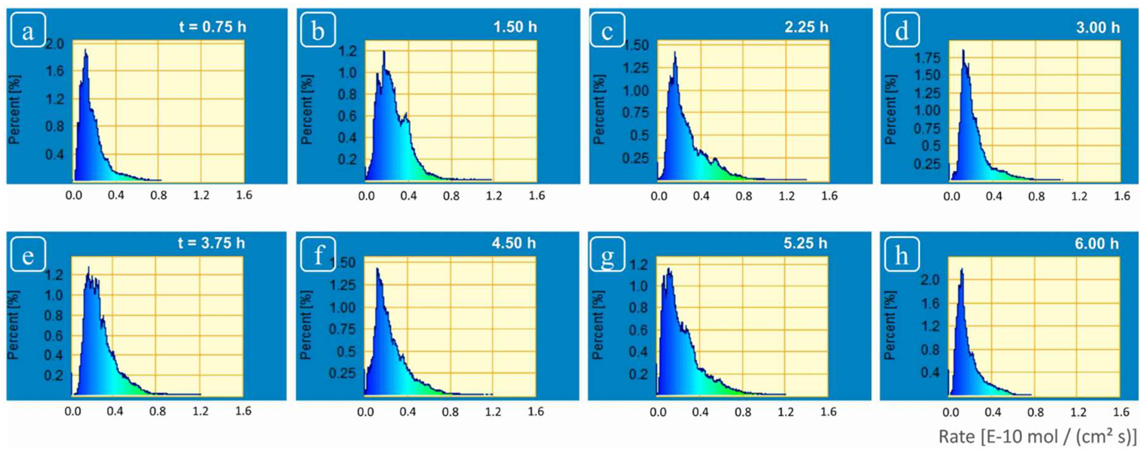
Histogram analysis of flux maps in the reaction rate spectra can provide information about frequency of rate contributors over overall surface reaction rate. Figure 5 shows the corresponding sequence of rate spectra obtained by using the difference map data shown in Figure 4. These rate spectra contain two types of information. First, the shape of the function (single peak versus discrete peaks) is relevant to surface energy range and distribution; second, the peak heights provide information about the frequency of distinct energetic sites [32]. The overall calculated rate ranges between ≤0.1 × 10⁻¹⁰ mol·cm⁻²·s⁻¹ and ≥1.4 × 10⁻¹⁰ mol·cm⁻²·s⁻¹ (Figure 5). The highest peak (frequency maximum, a single discrete peak) corresponds to the largest number of surface sites and represents the lowest rates (i.e., ~0.15 × 10⁻¹⁰ mol·cm⁻²·s⁻¹, Figure 5). The highest rates (>0.4 × 10⁻¹⁰ mol·cm⁻²·s⁻¹, green colors towards the tail of the spectrum) correspond to the retreat from highly reactive sites; for example, large, deep etch pits at screw dislocations in the central part of the calcite crystal (Figure 5a) and from the super-step feature.

After the completion of second reaction interval (1.5 h), a secondary peak of higher rates appears and reaches its maximum frequency (Figure 5b). This enhanced contribution of higher rates also leads to an increase in the highest observed rate, from 0.8 × 10⁻¹⁰ mol·cm⁻²·s⁻¹ (Figure 5a) to 1.2 × 10⁻¹⁰ mol·cm⁻²·s⁻¹ (Figure 5b). Enhanced activity at highly reactivity sites (etch pits at screw dislocations and the super-step) continues in the third reaction interval, leading to further increase in the maximum observed rate to 1.4 × 10⁻¹⁰ mol·cm⁻²·s⁻¹ (Figure 5c). In the fourth reaction interval, the height of frequency maximum increases again, however secondary rate contributions are reduced significantly, leading to a reduction in the maximum dissolution rate (Figure 5d). However, higher rates increased again during the fifth interval as indicated by reappearance of secondary peaks along tail end of the rate spectrum (Figure 5e). Significantly, the rate spectrum after the eighth or last reaction interval (Figure 5h) showed the highest rate of the order of ~0.8 × 10⁻¹⁰ mol·cm⁻²·s⁻¹ that was similar to those observed after the first reaction interval (Figure 5a).

3.2. Evolution of Surface Topography

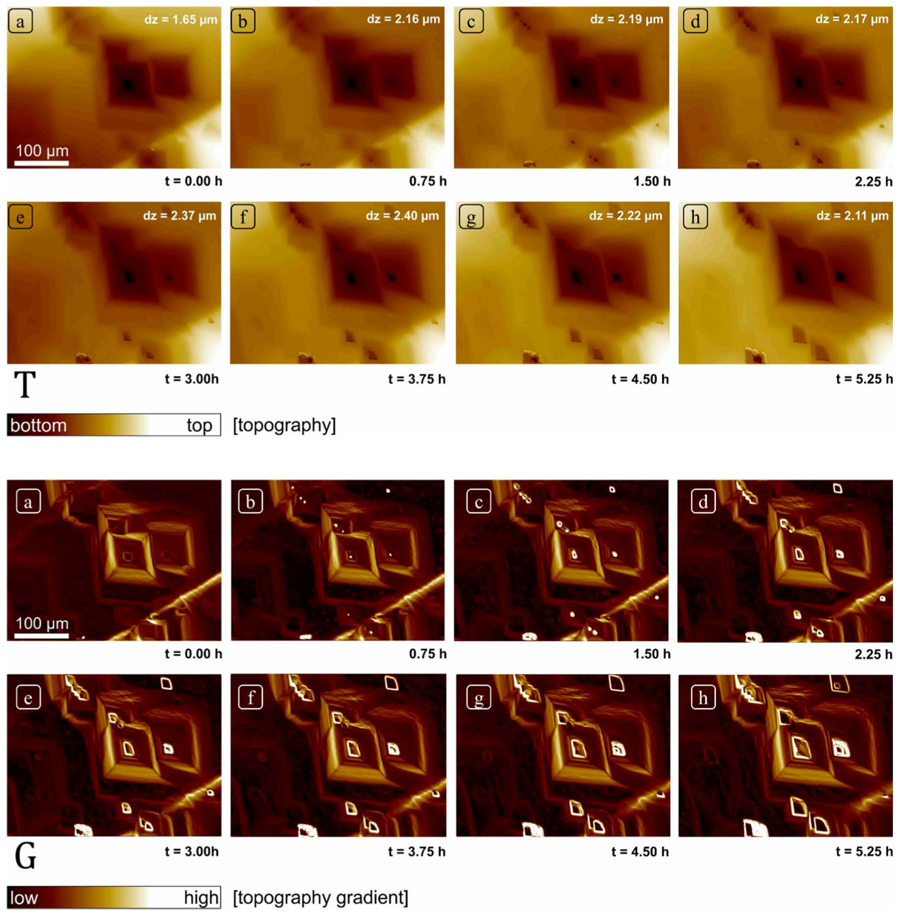
Where Figure 4 and Figure 5 detail rates distribution over the surface over a time interval, Figure 6 shows how absolute topography (Figure 6T) and surface gradient (Figure 6G) change as a series of snapshots, corresponding to the start of each time step in Figure 4 and Figure 5, beginning with t = 0 h (Figure 6T(a)), and ending at t = 5.25 h (Figure 6T(h)). In Figure 6T, the total height range associated with the color bar is also given ($dz=\dots$), and the lateral and vertical expansion of etch pits with reaction time is clearly observable in this sequence. With continued reaction, new etch pits can clearly be seen to nucleate to the northwest of the largest pits, giving rise to complex coalescence, and the super-step can be seen to migrate towards the southeast. The nucleation of these new pits is even more salient in gradient maps (Figure 6G), demonstrating how the spatial derivative easily identifies the nucleation and growth of new etch pits, regardless of the nature of the generating defect. These data confirm the simultaneous growth and nucleation of etch pits at screw dislocations in tandem with shallow, monolayer pits on terraces whose rapid coalescence also generates surface normal retreat.

4. Discussion

These data illustrate several important aspects of crystal dissolution kinetics. First, as has been demonstrated previously in many AFM and VSI studies, the instantaneous dissolution rate is clearly variable over the crystal surface, attaining maxima in deep etch pits whose morphology is consistent with screw dislocations, and its minima over terrace sites traversed by steps associated with screw dislocations (step waves) as well as shallow pits likely nucleated at point defects (see [33]). However, in addition to showing how these processes are simultaneously distributed over a significant area of the crystal surface, these data also record rate variation for a significant period in fine grained temporal detail, an aspect not addressed in many of our previous papers on calcite dissolution (e.g., see ref. [1]). Our data are consistent with step velocities and other AFM data pertaining to calcite dissolution are consistent to the extent that dissolution occurs at monolayer steps [11].

However, these data also show, quite serendipitously, that the range of rates and associated morphologic features one observes on the surface, may indeed reflect how long one spends observing it. We suggest that our super-step feature is likely a result of convergence of intersecting ${\left[48\overline{1}\right]}_{-}$ and ${\left[\overline{4}41\right]}_{+}$ steps, roughly parallel to $\left[22\overline{1}\right]$ and moving normal to $\left[010\right]$ directions. Such a feature is clearly not a step itself, but the complex, dynamic product of a large number of coalescent etch pits, thus requiring both significant time to develop, and demanding that dissolution operate over a significant area as well. We cannot assess the distribution of such features. Their transit over the surface removes significant amounts of material very efficiently, recording dissolution fluxes competitive with or exceeding screw dislocations (although clearly related to them genetically), but their lifetime may also be quite limited. Nevertheless, our point is that such phenomena are clearly highly scale- and time-dependent.

As reported previously in many surface investigations on calcite under similar experimental conditions, calcite crystal dissolved by the formation of rhombohedral etch pits [5,7,11,15]. The size of these pits was highly variable. Other than these well-developed features, the formation of several small and shallow etch pits was also observed. The reactivity of all these surface features was observed to vary as a function of time, however these changes do not point to any consistent, linear change in reactivity over time.

The heterogeneity of the surface reaction rates at the spatial scale also points to the operation of concurrent reaction mechanisms, as opposed to a single mechanism assumed in “mean rate” method. This conclusion rules out the use of a mean rate for predicting long-term dissolution behavior of mineral materials. Rate spectra [1] preserving contribution from all reaction mechanisms as range of rates, rather than a mean value.

4.1. On Spatial Rate Variability

The rate spectra obtained revealed a wide variability in rate distribution ranging from the highest rates (from highly reactive sites due to screw dislocations located at deep etch pits and macro-step surface) versus the slowest rates (from regions of slow reactivity, terrace sites) (Figure 5 and Figure 6). A wide range in spatial rates was observed from these experiments: between 0.03 × 10⁻¹⁰ mol·cm⁻²·s⁻¹ and 1.4 × 10⁻¹⁰ mol·cm⁻²·s⁻¹ (Figure 4). This range covers almost all the different values of calcite dissolution rates obtained under similar solution conditions in previous studies [15]. The spatial rate variability of crystalline material has also been reported in some previous investigations. For example, Arvidson et al. [15] reported large variation in distribution of etch pits and hence a potentially large variation in reactivity of a calcite crystal in a VSI monitored investigation. These authors further demonstrated that attainment of steady state in a dissolution experiment was rather a fortuitous occurrence, as the surface rates were dependent on the nucleation; widening and deepening of etch pits, which is a continuous process. The attainment of a steady state/constant rate, with insignificant variation would require a constant dislocation density which may not be easily fulfilled.

From the differences in absolute rates of two calcite samples (a large single crystal and a microcrystalline calcite) under exactly similar experimental conditions, Fischer et al. [1] ascribed the rate variability to differences in surface reactivity of the two samples. Moreover, there were also significant differences in distribution of these surface rates from two calcite samples. For instance, the highest rates were contributed by screw dislocations located at center of rarely found deep etch pits and the lowest rates were contributed by large number of shallow etch pits on single crystal calcite. These authors further commented that the averaging of such enormously variable rates to render a single mean value was misleading and inappropriate as the mean rate would inadequately represent the range of rates or the diversity of mechanisms [1].

4.2. On Temporal Rate Variability

There are two major reasons why the temporal surface rate variability was not addressed significantly in earlier microscopic rate investigations: (i) majority of the studies on morphologic evolution of dissolving crystals and the quantification of associated dissolution rates were carried out via AFM, which has a severe limitation of small scan area, and (ii) surface rate measurement was not accomplished at frequent intervals to establish any changes in the surface reactivity and derived dissolution rates with reaction progress [4,11].

In this study, we resolved the issue of temporal rate variability of calcite through frequently measured rates (after every 5 min) and surface topography changes using VSI. The dataset presented here is unique as it comprises of a set of frequently collected observations over a large surface area (414 × 313 µm²) of calcite crystal, which was large enough to observe the evolution of a large variety of features (monolayer etch pits, multilayer etch pits, screw dislocations, macro-step) through long experimental duration (6 h) on a pre-dissolved single crystal.

There are only few studies where the problem of temporal variability in surface reactivity was discussed to an appreciable extent due to the limitations associated with the use of AFM for these surface studies (as discussed in previous sections). For example, from K-feldspar surface rate measurements, Pollet-Villard et al. [34] found that despite increased etch pit distribution, surface retreat was a linear function of time. Furthermore, these authors reached the conclusion that anisotropic mineral reactivity lead to a continuous modification of the dissolution rate as a function of reaction time. Pollet-Villard et al. [34] also concluded that because of a significant variation in (intrinsic) surface reactivity, it was inappropriate to use the “mean rate” approach to quantify the reactivity of crystalline materials. In contrast, some researchers have reported an intrinsic decrease of long-term dissolution rate of the considered surface due to the development of pit walls with lower surface energy [35,36].

Although we observed changes in distribution of reactivity, no systematic, secular change in reactivity could be established (Figure 5 and Figure 6). These reactivity differences are thus related to structurally controlled factors at the mineral-water interface, characteristic of a complex and heterogeneous crystal surface.

4.3. Interpretation of Reaction Mechanism via Rate Spectral Analysis

The statistical analysis of the flux and rate maps in the frequency domain generates spectra that are linked to surface reaction mechanism (Figure 5), although this linkage is not well understood. Nevertheless, the spectral representation of rate maps (“rate spectra”, [1]) does preserve the contribution of all surface features to the overall rate [25], and has seen limited but increasing adoption in the literature [12,17]. It can be clearly seen in Figure 5 that the spectra generated from calcite dissolution rate maps (see also Figure 4) are an asymmetric distribution, one that is consistent with a heterogeneous, Boltzmann distribution of reactive surface sites. These results showed the dynamic nature of calcite surface which after interaction of several hours with fluid maintained the inherent variability and did not show attainment of surface rate stability. The asymmetry exhibited by these rate spectra was related to the presence of surface sites with huge variations in reactivity, i.e., poorly reactive sites (devoid of screw dislocations); and highly reactive sites (deep etch pits, super-step surface) on the other hand. Based on these results, we could not demonstrate any spatial dependence, however, it would be more accurate to relate these changes to the intrinsic heterogeneity of the crystal surface (which is discussed in detail in some recent investigations on surface dissolution kinetics by Luttge et al. [24].

Several studies have recently indicated the fundamental variability of mineral surface rates, mainly due to the occurrence of heterogeneous reactive surface sites [1,12,37,38]. A detailed discussion on heterogeneity of mineral surfaces and its relationship with surface rate variability could be found in a recent review [25]. A major conclusion that has been reached in current and several recent investigations on surface rates is that, instead of considering a mean rate, a stochastic treatment of dissolution kinetics should be preferred where a rate distribution constituting all the possible rate ranges is reported [24].

5. Conclusions

In this study, we present a unique set of VSI observations from the dissolution of a single calcite sample. This near in situ dissolution experiment provided insights on evolution of the surface morphology of a pre-dissolved calcite surface under alkaline solution conditions. By combining the carefully collected VSI data and its quantitative analysis using newly introduced rate spectra approach, we demonstrate that development of a large diversity of coevolving reactive surface features, e.g., ranging from nucleation, growth and annihilation of shallow pits (nm), long term development of complex, deep screw dislocations (d > 1 µm) and poorly understood super-steps (~1 µm) is responsible for the highly variable reaction rates of calcite in this long-term experiment.

Calcite continued to retreat and showed potential variability in reactivity of different surface sites on spatial and temporal scales. Sites that contributed the highest rates were those associated with deep, nested etch pits and the super-step feature. Slower rates were contributed by shallow or newly evolving monolayer etch pits. On this highly dynamic surface the integrated flux of these interacting processes contributes to a spectrum of rates. These asymmetric rate spectra do not reflect a single, dominant, reaction mechanism and are also variable in time and space.

Our VSI data demonstrated no specific trend of surface rate with reaction time. Variability in reactivity of the surface sites could be more realistically related to inherent heterogeneity of the crystal surface. The results also indicate towards the complexity of surface reactions which could not be oversimplified by taking simple means of the reaction rate at any given time step. Thus a stochastic treatment of dissolution kinetics should be preferred over deriving simple means from rate data to preserve the individual contribution of these highly variable surface sites to the overall rate.

References

- Fischer, C.; Arvidson, R.S.; Luttge, A. How predictable are dissolution rates of crystalline material? Geochim. Cosmochim. Acta 2012, 98, 177–185. [Google Scholar] [CrossRef]
- Morse, J.W.; Arvidson, R.S. The dissolution kinetics of major sedimentary carbonate minerals. Earth Sci. Rev. 2002, 58, 51–84. [Google Scholar] [CrossRef]
- Fischer, C.; Luttge, A. Pulsating dissolution of crystalline matter. Proc. Nat. Academy Sci. 2018. [Google Scholar] [CrossRef] [PubMed]
- Arvidson, R.S.; Morse, J.W. Formation and Diagenesis of Carbonate Sediments, In Treatise on Geochemistry, 2nd ed.; Elsevier Ltd.: Amsterdam, the Netherlands, 2014; Volume 9, pp. 61–101. [Google Scholar]
- Ruiz-Agudo, E.; Putnis, C.V.; Jimenez-Lopez, C.; Rodriguez-Navarro, C. An AFM study of calcite dissolution in concentrated saline solutions: The role of magnesium ions. Geochim. Cosmochim. Acta 2009, 73, 3201–3217. [Google Scholar] [CrossRef]
- Hillner, P.E.; Gratz, A.J.; Manne, S.; Hansma, P.K. Atomic-scale imaging of calcite growth and dissolution in real time. Geology 1992, 20, 359–362. [Google Scholar] [CrossRef]
- Dove, P.M.; Platt, F.M. Compatible real-time rates of mineral dissolution by Atomic Force Microscopy (AFM). Chem. Geol. 1996, 127, 331–338. [Google Scholar] [CrossRef]
- Liang, Y.; Baer, D.R.; McCoy, J.M.; Amonette, J.E.; Lafemina, J.P. Dissolution kinetics at the calcite-water interface. Geochim. Cosmochim. Acta 1996, 60, 4883–4887. [Google Scholar] [CrossRef]
- Liang, Y.; Baer, D.R.; McCoy, J.M.; Lafemina, J.P. Interplay between step velocity and morphology during the dissolution of CaCO3 surface. J. Vac. Sci. Technol. A 1996, 14, 1368–1375. [Google Scholar] [CrossRef]
- Jordan, G.; Higgins, S.R.; Eggleston, C.M.; Knauss, K.G.; Schmahl, W.W. Dissolution kinetics of magnesite in acidic aqueous solution, a hydrothermal atomic force microscopy (HAFM) study: Step orientation and kink dynamics. Geochim. Cosmochim. Acta 2001, 65, 4257–4266. [Google Scholar] [CrossRef]
- Ruiz-Agudo, E.; Putnis, C.V. Direct observations of mineral-fluid reactions using atomic force microscopy: The specific example of calcite. Mineral. Mag. 2012, 76, 227–253. [Google Scholar] [CrossRef]
- Emmanuel, S. Mechanisms influencing micron and nanometer-scale reaction rate patterns during dolostone dissolution. Chem. Geol. 2014, 363, 262–269. [Google Scholar] [CrossRef]
- Luttge, A.; Bolton, E.W.; Lasaga, A.C. An interferometry study of the dissolution kinetics of anorthite: The role of reactive surface area. American Journal of Science 1999, 299, 652–678. [Google Scholar] [CrossRef]
- Luttge, A.; Winkler, U.; Lasaga, A.C. Interferometric study of the dolomite dissolution: a new conceptual model for mineral dissolution. Geochim. et Cosmochim. Acta 2003, 67, 1099–1116. [Google Scholar] [CrossRef]
- Arvidson, R.S.; Ertan, I.E.; Amonette, J.E.; Luttge, A. Variation in calcite dissolution rates: A fundamental problem. Geochim. Cosmochim. Acta 2003, 67, 1623–1634. [Google Scholar] [CrossRef]
- Daval, D.; Hellmann, R.; Saldi, G.D.; Wirth, R.; Knauss, K.G. Linking nm-scale measurements of the anisotropy of silicate surface reactivity to macroscopic dissolution rate laws: New insights based on diopside. Geochim. Cosmochim. Acta 2013, 107, 121–134. [Google Scholar] [CrossRef] [Green Version]
- Brand, A.S.; Feng, P.; Bullard, J.W. Calcite dissolution rate spectra measured by in situ digital holographic microscopy. Geochim. Cosmochim. Acta 2017, 213, 317–329. [Google Scholar] [CrossRef] [PubMed]
- Liang, Y.; Baer, D.R. Anisotropic dissolution at the CaCO3()-water interface. Surf. Sci. 1997, 373, 275–287. [Google Scholar] [CrossRef]
- De Leeuw, N.H.; Parker, S.C.; Harding, J.H. Molecular dynamics simulation of crystal dissolution from calcite steps. Phys. Rev. B Condens. Matter Mater. Phys. 1999, 60, 13792–13799. [Google Scholar] [CrossRef]
- De Leeuw, N.H.; Parker, S.C. Modeling absorption and segregation of magnesium and cadmium ions to calcite surfaces: Introducing MgCO3 and CdCO3 potential models. J. Chem. Phys. 2000, 112, 4326–4333. [Google Scholar] [CrossRef]
- Kerisit, S.; Parker, S.C.; Harding, J.H. Atomistic simulation of the dissociative adsorption of water on calcite surfaces. J. Phys. Chem. B 2003, 107, 7676–7682. [Google Scholar] [CrossRef]
- Kurganskaya, I.; Luttge, A. Kinetic Monte Carlo approach to study carbonate dissolution. J. Phys. Chem. C 2016, 120, 6482–6492. [Google Scholar] [CrossRef]
- Jordan, G.; Rammensee, W. Dissolution rates of calcite (1014) obtained by scanning force microscopy: Microtpography-based dissolution kinetics on surfaces with anisotropic step velocities. Geochim. Cosmochim. Acta 1998, 62, 941–947. [Google Scholar] [CrossRef]
- Luttge, A.; Arvidson, R.S.; Fischer, C. A stochastic treatment of crystal dissolution kinetics. Elements 2013, 9, 183–188. [Google Scholar] [CrossRef]
- Fischer, C.; Kurganskaya, I.; Schafer, T.; Luttge, A. Variability of crystal surface reactivity: What do we know? Appl. Geochem. 2014, 43, 132–157. [Google Scholar] [CrossRef]
- Söngen, H.; Nalbach, M.; Adam, H. Kühnle, A. Three-dimensional atomic force microscopy mapping at the solid-liquid interface with fast and flexible data acquisition. Rev. Sci. Instrum. 2016, 87, 063704. [Google Scholar] [CrossRef] [PubMed]
- Miyata, K.; Tracey, J.; Miyazawa, K.; Haapasilta, V.; Spijker, P.; Kawagoe, Y.; Foster, A.S.; Tsukamoto, K.; Fukuma, T. Dissolution processes at step edges of calcite in water investigated by high-speed frequency modulation atomic force microscopy and simulation. Nano Lett. 2017, 17, 4083–4089. [Google Scholar] [CrossRef] [PubMed]
- Lasaga, A.C.; Luttge, A. Variation of calcite dissolution rate based on a dissolution stepwave model. Science 2001, 291, 2400–2404. [Google Scholar] [CrossRef] [PubMed]
- Arvidson, R.S.; Luttge, A. System and Method of Fluid Exposure and Data Acquisition. US Patent No. 8164756, 24 April 2012. United States Patent and Trademark Office. [Google Scholar]
- Vinson, M.D.; Luttge, A. Multiple length-scale kinetics: An integrated study of calcite dissolution rates and strontium inhibition. Am. J. Sci. 2005, 305, 119–146. [Google Scholar] [CrossRef]
- Luttge, A.; Arvidson, R.S. Reactions at surfaces: A new approach integrating interferometry and kinetic simulations. J. Am. Ceram. Soc. 2010, 93, 3519–3530. [Google Scholar] [CrossRef]
- Fischer, C.; Luttge, A. Beyond the conventional understanding of water-rock reactivity. Earth Planet. Sci. Lett. 2017, 457, 100–105. [Google Scholar] [CrossRef]
- Luttge, A.; Arvidson, R.S.; Fischer, C. Kinetic concepts for quantitative prediction of fluid-solid interactions. Chem. Geol. 2018. in review. [Google Scholar]
- Pollet-Villard, M.; Daval, D.; Ackerer, P.; Saldi, G.D.; Wild, B.; Knauss, K.G.; Fritz, B. Does crystallographic anisotropy prevent the conventional treatment of aqueous mineral reactivity? A case study based on K-feldspar dissolution kinetics. Geochim. Cosmochim. Acta 2016, 190, 294–308. [Google Scholar] [CrossRef]
- Godinho, J.R.A.; Piazolo, S.; Balic-Zunic, T. Importance of surface structure on dissolution of fluorite: Implications for surface dynamics and dissolution rates. Geochim. Cosmochim. Acta 2014, 126, 398–410. [Google Scholar] [CrossRef]
- Smith, M.E.; Knauss, K.G.; Higgins, S.R. Effects of crystal orientation on the dissolution of calcite by chemical and microscopic analysis. Chem. Geol. 2013, 360–361, 10–21. [Google Scholar] [CrossRef]
- Harries, D.; Pollok, K.; Langenhorst, F. Oxidative dissolution of 4C- and NC-pyrrhotite: Intrinsic reactivity differences, pH dependence, and the effect of anisotropy. Geochim. Cosmochim. Acta 2013, 102, 23–44. [Google Scholar] [CrossRef]
- Morse, J.W.; Arvidson, R.S.; Luttge, A. Calcium carbonate formation and dissolution. Chem. Rev. 2007, 107, 342–381. [Google Scholar] [CrossRef] [PubMed]
Figure 1.
Fluid cell operation. (A) Principal cell components include input flow port (q), scavenging pump port (s), capillary vacuum aspirator (v), and N2 dry gas line (g). Sample crystal is positioned under the optic path (o) of the Mirau interferometric objective (m). During reaction (B), fluid is introduced through the flow port and fills the volume bounded by the O-ring, immersing the sample crystal. The scavenging port is closed, and fluid is removed by the vacuum aspirator, whose lateral position controls the height of the fluid envelope. Input flow rate is sufficient for rapid exchange within the cell’s open volume. Prior to data collection (C), the input port is closed and scavenging port is opened, allowing fluid to drain rapidly from the cell. The sample surface is simultaneously dried via N2. Once data collection is completed, the cell is returned to flow configuration (B). Total cycle time is 20–30 s [29].
Figure 2.
Visualization of rate data correction due to surface normal retreat of smooth surface plateaus. The precision of the instrument would allow for a reproducibility that is defined by the difference between the blue-colored and the gray-colored rate curves.
Figure 3.
False color height map of surface at onset of reaction sequence, showing well-developed etch pits (“S”), terraces (“T”), and super-step feature (“M”) discussed in text. Field of view 413.6 × 313.3 µm2, 20× Mirau objective, 20 µm horizontal scale bar, total height range 1.7 µm. Note that the intercept of the interferometer’s height scale is arbitrarily set, and negative versus positive values are simply heights relative to a datum, and do not imply growth or otherwise positive changes in surface elevation. Comparisons of height data obtained at various reaction times (e.g., subtraction or difference maps) compute a pairwise correction in these intercepts to yield a consistent analysis (see discussion in text).
Figure 4.
Rate maps of calcite reacted surface after reaction intervals ranging between 0.75 h and 6 h (a–h). Obtuse steps associated with deep etch pits propagate to the north and east, acute steps to the south and west, respectively, from their associated dislocation centers. See text for description.
Figure 5.
Rate spectra sequence showing spatial and temporal heterogeneity of dissolution rates of calcite surface after reaction intervals ranging between 0.75 h and 6 h (a–h). Although the horizontal scale (rate) is fixed, note that the y-scale is variable.
Figure 6.
Reaction sequence data. Height (T, top) and gradient (G, bottom) maps of calcite surface prior to the reaction (a) and after reaction duration of 0.75 h to 5.25 h (b–h).
© 2018 by the authors. Licensee MDPI, Basel, Switzerland. This article is an open access article distributed under the terms and conditions of the Creative Commons Attribution (CC BY) license (http://creativecommons.org/licenses/by/4.0/).
Share and Cite
MDPI and ACS Style
Bibi, I.; Arvidson, R.S.; Fischer, C.; Lüttge, A. Temporal Evolution of Calcite Surface Dissolution Kinetics. Minerals 2018, 8, 256. https://doi.org/10.3390/min8060256
AMA Style
Bibi I, Arvidson RS, Fischer C, Lüttge A. Temporal Evolution of Calcite Surface Dissolution Kinetics. Minerals. 2018; 8(6):256. https://doi.org/10.3390/min8060256
Chicago/Turabian StyleBibi, Irshad, Rolf S. Arvidson, Cornelius Fischer, and Andreas Lüttge. 2018. "Temporal Evolution of Calcite Surface Dissolution Kinetics" Minerals 8, no. 6: 256. https://doi.org/10.3390/min8060256
Note that from the first issue of 2016, this journal uses article numbers instead of page numbers. See further details here.