Review

Self-Gravitating Systems in Extended Gravity

by
Arturo Stabile
1,* and
Salvatore Capozziello
2,3,4,*
1
Dipartimento di Ingegneria, Università del Sannio, Palazzo Dell'Aquila Bosco Lucarelli, Corso Garibaldi, 107-82100 Benevento, Italy
2
Dipartimento di Fisica, Università di Napoli "Federico II", Complesso Universitario di Monte Sant'Angelo, Edificio G, Via Cinthia, I-80126 Napoli, Italy
3
INFN Sezione di Napoli, Complesso Universitario di Monte Sant' Angelo, Ed. G, Via Cinthia, I-80126 Napoli, Italy
4
Gran Sasso Science Institute (INFN), Via F. Crispi 7, I-67100 L' Aquila, Italy
*
Authors to whom correspondence should be addressed.
Galaxies 2014, 2(4), 520-576; https://doi.org/10.3390/galaxies2040520
Submission received: 21 July 2014 / Revised: 10 November 2014 / Accepted: 14 November 2014 / Published: 4 December 2014
(This article belongs to the Special Issue Beyond Standard Gravity and Cosmology)

Abstract

:
Starting from the weak field limit, we discuss astrophysical applications of Extended Theories of Gravity where higher order curvature invariants and scalar fields are considered by generalizing the Hilbert-Einstein action linear in the Ricci curvature scalar R. Results are compared to General Relativity in the hypothesis that Dark Matter contributions to the dynamics can be neglected thanks to modified gravity. In particular, we consider stellar hydrostatic equilibrium, galactic rotation curves, and gravitational lensing. Finally, we discuss the weak field limit in the Jordan and Einstein frames pointing out how effective quantities, as gravitational potentials, transform from one frame to the other and the interpretation of results can completely change accordingly.

1. Introduction

The today observed Universe appears spatially flat and undergoing an accelerated expansion. Several observational data probe this pictures [1,2,3,4,5,6] but two unrevealed ingredients are needed in order to achieve this dynamical scenario, namely Dark Matter (DM) at galactic and extragalactic scales and Dark Energy (DE) at cosmological scales. In particular, the dynamical evolution of self-gravitating structures can be figured out by the standard Newtonian gravity, but DM is needed to obtain agreement with observations [7].
On the other hand, the effort to give a physical explanation to the today observed cosmic acceleration has attracted a lot of interest in the so-called Extended Theories of Gravity [8,9,10], considered a viable mechanism to explain the cosmic acceleration by extending the geometric sector without introducing DM and DE. Other issues, at astrophysical level, can be framed in the same approach [11] and then, apart the cosmological dynamics, a systematic analysis of such theories urges at short scale and in the weak field limit. Extended Theories of Gravity are then a new paradigm for gravitational physics aimed to address shortcomings coming out at ultra-violet and infra-red scales.
While it is very natural to extend General Relativity (GR) to theories with additional geometric degrees of freedom, recent attempts focused on the old idea of modifying the gravitational Lagrangian in taking into account generic functions of curvature invariants and leading to higher-order field equations. Despite of the positive results of GR, the study of possible modifications of Einstein’s theory has a long history which reaches back to the early 1920s [12,13,14,15,16,17,18,19]. The proposed early amendments of Einstein’s theory were aimed toward the unification of gravity with the other interactions of physics. Besides, the presence of Big Bang singularity, the flatness and horizon problems [20] led to the statement that Cosmological Standard Model, based on GR and Standard Model of Particles, is inadequate to describe the universe in extreme regimes. From Quantum Field Theory point of view, GR is a classical theory which does not work at fundamental level in order to achieve a full and comprehensive quantum description of spacetime and gravity.
Despite of modifications, the spirit of GR should be preserved since the only effective request is that the Hilbert-Einstein action is not given a priori. This is the reason why one can deals with Extended Theories of Gravity and not with Alternative Gravity. One of the possibilities is that gravitational interaction could act in different ways at different scales. In any case, the robust results of GR, at local and Solar System scales, have to be preserved for consistency (see [21] for a detailed discussion). This is the case of f ( R ) -gravity which reduces, in principle, to GR as soon as f ( R ) R .
On the other hand, the strong gravity regime [22] is another way to check the viability of these theories. In general, the formation and the evolution of stars can be considered as suitable test-beds for Alternative Theories of Gravity. Considering the case of f ( R ) -gravity, divergences stemming from the functional form of f ( R ) may prevent the existence of relativistic stars in these theories [23]. There are also numerical solutions corresponding to static star configurations with strong gravitational fields [24,25] where the choice of the equation of state is crucial for the existence of solutions.
Some observed stellar systems are incompatible with the standard models of stellar structure. We refer to anomalous neutron stars, the so called “magnetars” [26] with masses larger than their expected Volkoff mass. It seems that, on particular length scales, the gravitational force is larger or smaller than the corresponding GR value [27,28].
A lot of research work is pointing out that physics of compact objects could be the experimentum crucis to retain or rule out Alternative Theories of Gravity since precise observational data could give extremely good signatures for the models (see for example [29,30,31,32,33,34,35,36,37,38]).
Other motivations to modify gravity come from the issue of a full recovering of the Mach principle which leads to assume a varying gravitational coupling. The principle states that the local inertial frame is determined by the averaging process of motion of distant astronomical objects [40]. This fact implies that the gravitational coupling can be scale-dependent and related to some scalar field. As a consequence, the concept of inertia and the Equivalence Principle have to be revised. For example, the Brans-Dicke theory [41] is a preliminary attempt to define an alternative theory of gravity: it takes into account a variable Newton gravitational coupling, whose dynamics is governed by a scalar field non-minimally coupled to the geometry. In such a way, Mach’s principle is better implemented [41,42,43].
As already mentioned, corrections to the gravitational Lagrangian were already considered by several authors [13,16,17] soon after the GR was proposed. From a conceptual viewpoint, there are no reason a priori to restrict the gravitational Lagrangian to a linear function of the Ricci scalar, minimally coupled with matter [44]. Since all curvature invariants are at least second order differential, the corrective terms in the field equations will be always at least fourth order. That is why one calls them higher order terms (with respect to GR).
Due to the increasing complexity of the field equations, the main amount of works is related to achieve some formally equivalent theories, where the reduction of the order of field equations can be obtained by considering metric and connections as independent fields [44,45,46,47,48]. In addition, many authors exploited the formal relation to scalar-tensor theories to make some statements about the weak field regime [49]. Moreover other authors discussed a systematic analysis of such theories in the low energy limit [49,50,51,52,53,54,55,56,57,58,59]. In particular, Fourth Order Gravity has been studied in the Newtonian limit (weak field and small velocity) and in the Minkowskian limit (e.g., gravitational waves) [60]. In the former case, one finds modifications of gravitational potential, while in the latter, massive gravitational wave modes come out [61].
However, the weak field limit of such theories have to be tested against realistic self-gravitating structures. Galactic rotation curves, stellar hydrodynamics and gravitational lensing appear natural candidates as test-bed experiments [62,63,64,65].
In this paper, starting from Newtonian and post-Newtonian approximations of Extended Gravity, we match the outcomes with some typical astrophysical structures. The Newtonian limit of the general Fourth Order Gravity is considered by generalizing f ( R ) models with generic functions containing other curvature invariants, as Ricci square ( R α β R α β ) and Riemann square ( R α β γ δ R α β γ δ ). The spherically symmetric solutions of metric tensor yet present Yukawa-like behaviors, but, in general, one has two characteristic lengths. The Gauss-Bonnet invariant G = R 2 4 R μ ν R μ ν + R μ ν λ σ R μ ν λ σ , and the Weyl invariant C α β γ δ C α β γ δ can be reduced to the above cases.
The plan of the review is the following. In Section 2 we summarize the basic ingredients of the Newtonian and the post-Newtonian limits [56]. Section 3 is devoted to the Newtonian limit of Fourth Order Gravity [57], while, in Section 3.1, we discuss the solutions generated by pointlike sources with and without gauge conditions. A brief analysis of the free parameters of the theory is performed.
In Section 4.1 we briefly review the classical hydrostatic problem for stellar structures and in Section 4.2 we derive the modified Poisson equation in the framework of the Newtonian limit of f ( R ) -gravity. Then the modified Lané-Emden equation is obtained in Section 4.3. Analytic and numerical solutions are discussed [66].
Galactic rotation curves are considered in Section 5. The main properties of galactic metric are discussed and, in particular, the violation of the Gauss theorem due to the corrections to the Newtonian potential. In Section 5.1, we discuss models for the mass distribution of galactic components. A qualitative and quantitative comparison between the experimental data and the theoretical predictions of rotation curve [65] is obtained for our Galaxy and for NGC 3198 in Section 5.2 by fixing numerically the free parameters of the theory. The motion of massive particles is discussed in Section 5.3: analogies and differences between general Fourth Order Gravity and R n -gravity are pointed out. Fourth Order Gravity is also considered with and without DM. The outcomes are compared with GR. The rotation curves results higher or lower than the same curves in GR, if the squared Ricci scalar contribution is dominant or not with respect to the contribution of the squared Ricci tensor. However, by modifying gravity, also the spatial description of DM could undergoes modifications and the free parameters of model assume different values.
Gravitational lensing is analyzed in the case of pointlike sources (Section 6.1) and extended sources (Section 6.2). An important outcome is found in the case of thin lenses: the bending of photons in f ( R ) -gravity is the same as in GR [67,68]. If we add the squared Ricci tensor contribution, we obtain a shift of the image positions (Section 6.3).
Finally we take into account the weak field limit of scalar-tensor gravity [69] in the Jordan frame (Section 7.1) and compare it with the analogous in the Einstein frame (Section 7.2). Specifically, we consider how physical quantities, like gravitational potentials, derived in the Newtonian approximation for the same scalar-tensor theory, behave in the Jordan and in the Einstein frame. The approach allows to discriminate features that are invariant under conformal transformations and gives contributions in the debate of selecting the true physical frame.The particular case of f ( R ) -gravity is considered in Section 7.3.
Discussions and conclusions are drawn in Section 8.

2. Newtonian and Post-Newtonian Approximations

It is worth discussing some general issues on the Newtonian and post-Newtonian limits. Basically there are some general features one has to take into account when approaching these limits, whatever the underlying theory of gravitation is.
If one consider a system of gravitationally interacting particles of mass M ¯ , the kinetic energy 1 2 M ¯ v ¯ 2 will be, roughly, of the same order of magnitude as the typical potential energy U = G M ¯ 2 / r ¯ , with M ¯ , r ¯ , and v ¯ the typical average values of masses, separations, and velocities of these particles. As a consequence:
v 2 ¯ G M ¯ r ¯
(for instance, a test particle in a circular orbit of radius r about a central mass M will have velocity v given in Newtonian mechanics by the exact formula v 2 = G M / r ).
The post-Newtonian approximation can be described as a method for obtaining the motion of the system to higher than first order (approximation which coincides with the Newtonian mechanics) with respect to the quantities G M ¯ / r ¯ and v ¯ 2 assumed small with respect to the squared light speed c 2 . This approximation is sometimes referred to as an expansion in inverse powers of the light speed.
The typical values of the Newtonian gravitational potential U are nowhere larger than 10 5 in the Solar System (in geometrized units, U / c 2 is dimensionless). On the other hand, planetary velocities satisfy the condition v ¯ 2 U , while (We consider here on the velocity v in units of the light speed c) the matter pressure p experienced inside the Sun and the planets is generally smaller than the matter gravitational energy density ρ U , in other words (Typical values of p / ρ are ∼ 10 5 in the Sun and ∼ 10 10 in the Earth [70]) p / ρ U . Furthermore one must consider that even other forms of energy in the Solar System (compressional energy, radiation, thermal energy, etc.) have small intensities and the specific energy density Π (the ratio of the energy density to the rest-mass density) is related to U by Π U (Π is ∼ 10 5 in the Sun and ∼ 10 9 in the Earth [70]). As matter of fact, one can consider that these quantities, as function of the velocity, give second order contributions
U v 2 p / ρ Π O ( )
Therefore, the velocity v gives O ( 1 ) terms in the velocity expansions, U 2 is of order O ( 4 ) , U v of O ( 3 ) , U Π is of O ( 4 ) , and so on. Considering these approximations, one has
t v ·
and
| / t | | | O ( 1 )
Now, particles move along geodesics
d 2 x μ d s 2 + Γ σ τ μ d x σ d s d x τ d s = 0
where d s = g α β d x α d x β is the relativistic distance. The Equation (5) can be written in details as
d 2 x i d t 2 = Γ t t i 2 Γ t m i d x m d t Γ m n i d x m d t d x n d t + Γ t t t + 2 Γ t m t d x m d t + 2 Γ m n t d x m d t d x n d t d x i d t
where the set of coordinates adopted is x μ = ( t , x 1 , x 2 , x 3 ) . In the Newtonian approximation, that is vanishingly small velocities and only first-order terms in the difference between g μ ν and the Minkowski metric η μ ν , one obtains that the particle motion equations reduce to the standard result
d 2 x i d t 2 Γ t t i 1 2 g t t x i
The quantity 1 g t t is of order G M ¯ / r ¯ , so that the Newtonian approximation gives d 2 x i / d t 2 to the order G M ¯ / r ¯ 2 , that is, to the order v ¯ 2 / r . As a consequence if we would like to search for the post-Newtonian approximation, we need to compute d 2 x i / d t 2 to the order v ¯ 4 / r ¯ . Due to the Equivalence Principle and the differentiability of spacetime manifold, we expect that it should be possible to find out a coordinate system in which the metric tensor is nearly equal to the Minkowski one η μ ν , the correction being expandable in powers of G M ¯ / r ¯ v ¯ 2 . In other words one has to consider the metric developed as follows (The Greek index runs from 0 to 3; the Latin index runs from 1 to 3)
g t t ( t , x ) 1 + g t t ( 2 ) ( t , x ) + g t t ( 4 ) ( t , x ) + O ( 6 ) g t i ( t , x ) g t i ( 3 ) ( t , x ) + O ( 5 ) g i j ( t , x ) δ i j + g i j ( 2 ) ( t , x ) + O ( 4 )
where δ i j is the Kronecker delta, and for the controvariant form of g μ ν , one has
g t t ( t , x ) 1 + g ( 2 ) t t ( t , x ) + g ( 4 ) t t ( t , x ) + O ( 6 ) g t i ( t , x ) g ( 3 ) t i ( t , x ) + O ( 5 ) g i j ( t , x ) δ i j + g ( 2 ) i j ( t , x ) + O ( 4 )
In evaluating Γ α β μ we must take into account that the scale of distance and time, in our systems, are respectively set by r ¯ and r ¯ / v ¯ , thus the space and time derivatives should be regarded as being of order
x i 1 r ¯ , t v ¯ r ¯
Using the above approximations Equation (8) and Equation (9), we have, from the definition of Christoffel symbols Γ α β μ = 1 2 g μ σ ( g α σ , β + g β σ , α g α β , σ ) ,
Γ ( 3 ) t t t = 1 2 g t t ( 2 ) , t Γ ( 2 ) t t i = 1 2 g t t ( 2 ) , i Γ ( 2 ) j k i = 1 2 g ( 2 ) j k , i g ( 2 ) j , k i g ( 2 ) k , j i Γ ( 3 ) i j t = 1 2 g ( 3 ) i , j t + g ( 3 ) j , i t g ( 3 ) i j , t Γ ( 3 ) t j i = 1 2 g ( 3 ) t j , i g ( 3 ) t , j i g ( 2 ) j , t i Γ ( 4 ) 0 i 0 = 1 2 g ( 4 ) t , i t + g ( 2 ) t t g t t , i ( 2 ) Γ ( 4 ) t t i = 1 2 g ( 4 ) t t , i + g ( 2 ) i m g t t , m ( 2 ) 2 g ( 3 ) t , t i Γ ( 2 ) t i t = 1 2 g ( 2 ) t , i t
The Ricci tensor component are
R t t ( 2 ) = 1 2 g t t ( 2 ) R t t ( 4 ) = 1 2 g t t ( 4 ) 1 2 g ( 2 ) , m m n g t t , n ( 2 ) 1 2 g ( 2 ) m n g t t , m n ( 2 ) + 1 2 g ( 2 ) m , t t m 1 4 g ( 2 ) t t , m g t t , m ( 2 ) 1 4 g ( 2 ) m m , n g t t , n ( 2 ) g ( 3 ) t , m t m R t i ( 3 ) = 1 2 g t i ( 3 ) 1 2 g ( 2 ) i , m t m 1 2 g ( 3 ) t , m i m + 1 2 g ( 2 ) m , t i m R i j ( 2 ) = 1 2 g i j ( 2 ) 1 2 g ( 2 ) i , m j m 1 2 g ( 2 ) j , m i m 1 2 g ( 2 ) t , i j t + 1 2 g ( 2 ) m , i j m
with △ and ▽, respectively, the Laplacian and the gradient in flat space. The inverse of the metric tensor is defined by means of the equation
g α ρ g ρ β = δ β α
with δ β α the Kronecker delta. The relations among the higher than first order terms turn out to be
g ( 2 ) t t ( t , x ) = g t t ( 2 ) ( t , x ) g ( 4 ) t t ( t , x ) = g t t ( 2 ) ( t , x ) 2 g t t ( 4 ) ( t , x ) g ( 3 ) t i ( t , x ) = g t i ( 3 ) ( t , x ) g ( 2 ) i j ( t , x ) = g i j ( 2 ) ( t , x )
Finally the Lagrangian of a particle in presence of a gravitational field can be expressed as proportional to the invariant distance d s 1 / 2 , thus we have :
L = g ρ σ d x ρ d t d x σ d t 1 / 2 = g t t + 2 g t m v m + g m n v m v n 1 / 2 = 1 + g t t ( 2 ) + g t t ( 4 ) + 2 g t m ( 3 ) v m v 2 + g m n ( 2 ) v m v n 1 / 2
which, to the O ( 2 ) order, reduces to the classic Newtonian Lagrangian of a test particle L New = ( 1 + g t t ( 2 ) v 2 ) 1 / 2 , where v = d x m d t d x m d t . As matter of fact, post-Newtonian physics has to involve higher than O ( 4 ) order terms in the Lagrangian.
An important remark concerns the odd-order perturbation terms O ( 1 ) or O ( 3 ) . Since, these terms contain odd powers of velocity v or of time derivatives, they are related to the energy dissipation or absorption by the system. Nevertheless, the mass-energy conservations prevents the energy and mass losses and, as a consequence, prevents, in the Newtonian limit, terms of O ( 1 ) and O ( 3 ) orders in the Lagrangian. If one takes into account contributions higher than O ( 4 ) order, different theories give different predictions. GR, for example, due to the conservation of post-Newtonian energy, forbids terms of O ( 5 ) order; on the other hand, terms of O ( 7 ) order can appear and are related to the energy lost by means of the gravitational radiation.
On the matter side, i.e., right-hand side of the field equations we start with the general definition of the energy-momentum tensor of a perfect fluid with additional energy Π
T μ ν = ( ρ + Π ρ + p ) u μ u ν p g μ ν
The explicit form of the energy-momentum tensor can be derived as follows
T t t = ρ + ρ ( v 2 2 U + Π ) + ρ v 2 p ρ + v 2 + 2 V + Π + σ 2 Π U T t i = ρ v i + ρ [ v i ( p ρ + 2 V + v 2 + Π + h t i T i j = ρ v i v j + p δ i j + ρ v i v j Π + p ρ + 4 V + v 2 + 2 U 2 v c δ c ( i h 0 | j ) + 2 p V ρ δ i j
where ρ is the density of energy.

3. The Newtonian Limit of f ( X , Y , Z ) -Gravity

Let us start with a general class of fourth order theories given by the action
A = d 4 x g f ( X , Y , Z ) + X L m
where f is an unspecified function of curvature invariants X R , Y R α β R α β and Z R α β γ δ R α β γ δ . The term L m is the minimally coupled ordinary matter contribution. In the metric approach, the field equations are obtained by varying Equation (18) with respect to g μ ν . We get
H μ ν = f X R μ ν f 2 g μ ν f X ; μ ν + g μ ν f X + 2 f Y R μ α R α ν 2 [ f Y R α ( μ ] ; ν ) α + + [ f Y R μ ν ] + [ f Y R α β ] ; α β g μ ν + 2 f Z R μ α β γ R ν α β γ 4 [ f Z R μ α β ν ] ; α β = X T μ ν
where T μ ν = 1 g δ ( g L m ) δ g μ ν is the energy-momentum tensor of matter, f X = d f d X , f Y = d f d Y , f Z = d f d Z , = ; σ ; σ and X = 8 π G . The convention for Ricci’s tensor is R μ ν = R σ μ σ ν , while for the Riemann tensor is R α β μ ν = Γ β ν , μ α + . . . . The affinities are the usual Christoffel symbols of the metric. The adopted signature is ( + ) (for details, see [71]). The trace of field Equation (19) is the following
H = g α β H α β = f X R + 2 f Y R α β R α β + 2 f Z R α β γ δ R α β γ δ 2 f + + [ 3 f X + f Y R ] + 2 [ ( f Y + 2 f Z ) R α β ] ; α β = X T
where T = T σ σ is the trace of energy-momentum tensor.
Some authors considered a linear Lagrangian containing not only X, Y and Z but also the first power of curvature invariants R and R α β ; α β . Such a choice is justified because all curvature invariants have the same dimension ( L 2 ) [72]. Furthermore, this dependence on these two last invariants is only formal, since from the contracted Bianchi identity ( 2 R α β ; α β R = 0 ) we have only one independent invariant. In any linear theory of gravity (the function f is linear) the terms R and R α β ; α β give us no contribution to the field equations, because they are four-divergences. However, if we consider a function of R or R α β ; α β by varying the action we still could have the four-divergences but we would have the contributions of sixth order differential. For our aim (we want to stay in framework of fourth order differential equations) the most general theory of fourth order is the action Equation (18).
The Newtonian limit analysis starts from the development Equation (8) of the metric tensor. Then we set the metric as
g μ ν = 1 + g t t ( 2 ) ( t , x ) 0 0 δ i j + g i j ( 2 ) ( t , x ) +
where we note that the presence of function g i j ( 2 ) ( t , x ) is superfluous here for our aim but it will be fundamental about the gravitational lensing. The curvature invariants X, Y, Z become
X X ( 2 ) + X ( 4 ) + Y Y ( 4 ) + Y ( 6 ) + Z Z ( 4 ) + Z ( 6 )
The function f can be developed as
f ( X , Y , Z ) f ( 0 ) + f X ( 0 ) X ( 2 ) + 1 2 f X X ( 0 ) X ( 2 ) 2 + f X ( 0 ) X ( 4 ) + f Y ( 0 ) Y ( 4 ) + f Z ( 0 ) Z ( 4 ) +
and analogous relations for partial derivatives of f are obtained. From the interpretation of stress-energy tensor components Equation (17) as energy density, momentum density and momentum flux, we have T t t , T t i and T i j at the various orders
T t t = T t t ( 0 ) + T t t ( 2 ) + O ( 4 ) T t i = T t i ( 1 ) + O ( 3 ) T i j = T i j ( 2 ) + O ( 4 )
where T μ ν ( N ) denotes the term in T μ ν of order M ¯ / r ¯ 3 v ¯ N . In particular T t t ( 0 ) is the density of rest-mass, while T t t ( 2 ) is the non-relativistic part of the energy density.
From the lowest order of field Equation (19) we have
f ( 0 ) = 0
Not only in f ( R ) -gravity [55,56,73] but also in f ( X , Y , Z ) -theory a missing cosmological component in the action Equation (18) implies that the space-time is asymptotically Minkowskian. The Equation (19) and Equation (20) at O ( 2 ) —order become (We used the properties: 2 R α β ; α β R = 0 and R μ α β ν ; α β = R μ α ; ν α R μ ν )
H t t ( 2 ) = f X ( 0 ) R t t ( 2 ) [ f Y ( 0 ) + 4 f Z ( 0 ) ] R t t ( 2 ) f X ( 0 ) 2 X ( 2 ) [ f X X ( 0 ) + f Y ( 0 ) 2 ] X ( 2 ) = X T t t ( 0 ) H i j ( 2 ) = f X ( 0 ) R i j ( 2 ) [ f Y ( 0 ) + 4 f Z ( 0 ) ] R i j ( 2 ) + f X ( 0 ) 2 X ( 2 ) δ i j + [ f X X ( 0 ) + f Y ( 0 ) 2 ] X ( 2 ) δ i j + f X X ( 0 ) X ( 2 ) , i j + [ f Y ( 0 ) + 4 f Z ( 0 ) ] R m i , j m ( 2 ) + f Y ( 0 ) R m j , i m ( 2 ) = 0 H ( 2 ) = f X ( 0 ) X ( 2 ) [ 3 f X X ( 0 ) + 2 f Y ( 0 ) + 2 f Z ( 0 ) ] X ( 2 ) = X T ( 0 )
By introducing the quantities
m 1 2 f X ( 0 ) 3 f X X ( 0 ) + 2 f Y ( 0 ) + 2 f Z ( 0 ) m 2 2 f X ( 0 ) f Y ( 0 ) + 4 f Z ( 0 )
we get three differential equations for curvature invariant X ( 2 ) , t t - and i j -component of Ricci tensor R μ ν ( 2 )
( m 2 2 ) R t t ( 2 ) + m 2 2 2 m 1 2 + 2 m 2 2 6 m 1 2 X ( 2 ) = m 2 2 X f X ( 0 ) T t t ( 0 ) ( m 2 2 ) R i j ( 2 ) + m 1 2 m 2 2 3 m 1 2 i j 2 m 2 2 2 m 1 2 + 2 m 2 2 6 m 1 2 δ i j X ( 2 ) = 0 ( m 1 2 ) X ( 2 ) = m 1 2 X f X ( 0 ) T ( 0 )
The solution for curvature invariant X ( 2 ) in third line of Equation (28) is
X ( 2 ) ( t , x ) = m 1 2 X f X ( 0 ) d 3 x G 1 ( x , x ) T ( 0 ) ( t , x )
where G 1 ( x , x ) is the Green function of the field operator m 1 2 . The solution for g t t ( 2 ) , by remembering R t t ( 2 ) = 1 2 g t t ( 2 ) , is
g t t ( 2 ) ( t , x ) = 1 2 π d 3 x d 3 x G 2 ( x , x ) | x x | [ m 2 2 X f X ( 0 ) T t t ( 0 ) ( t , x ) ( m 1 2 + 2 m 2 2 ) X 6 f X ( 0 ) T ( 0 ) t , x ) + + m 2 2 m 1 2 6 X ( 2 ) ( t , x ) ]
where G 2 ( x , x ) is the Green function of the field operator m 2 2 .
The expression Equation (30) is the “modified” gravitational potential (here we have a factor 2) for f ( X , Y , Z ) -gravity. The solution for the gravitational potential Φ = g t t ( 2 ) / 2 has a Yukawa-like behaviors ([55,57]) depending by a characteristic lengths on whose it evolves.
The i j -component of Ricci tensor in terms of metric tensor Equation (12) can be expressed by using the harmonic gauge condition ( g α β Γ α β μ = 0 ) as R i j ( 2 ) | H G = 1 2 g i j , m m ( 2 ) = 1 2 g i j ( 2 ) . Then the general solution for g i j ( 2 ) from Equation (28), in the harmonic gauge, is
g i j ( 2 ) | H G = 1 2 π d 3 x d 3 x G 2 ( x , x ) | x x | m 1 2 m 2 2 3 m 1 2 i j 2 m 2 2 2 m 1 2 + 2 m 2 2 6 m 1 2 x δ i j X ( 2 ) ( x )
While if we hypothesize g i j ( 2 ) = 2 Ψ δ i j (We choose a system of isotropic coordinates. Generally the set of coordinates ( t , r , θ , ϕ ) are called standard coordinates if the metric is expressed as d s 2 = g t t ( t , r ) d t 2 + g r r ( t , r ) d r 2 r 2 d Ω while if one has d s 2 = g t t ( t , x ) d t 2 + g i j ( t , x ) d x i d x j the set ( t , x 1 , x 2 , x 3 ) is called isotropic coordinates [52,75]) we have (without the validity of the harmonic gauge condition) R i j ( 2 ) = Ψ δ i j + ( Ψ Φ ) , i j and the second field equation of Equation (28) becomes
Ψ = d 3 x G 2 ( x , x ) m 2 2 2 m 1 2 + 2 m 2 2 6 m 1 2 x X ( 2 ) ( x ) ( Φ Ψ ) , i j = m 1 2 m 2 2 3 m 1 2 d 3 x G 2 ( x , x ) X , i j ( 2 ) ( x )
Then the general solution for g i j ( 2 ) from Equation (28) is
g i j ( 2 ) = 2 Ψ δ i j = δ i j 2 π d 3 x d 3 x G 2 ( x , x ) | x x | m 2 2 2 m 1 2 + 2 m 2 2 6 m 1 2 x X ( 2 ) ( x )
and the second line of Equation (32) is mathematically satisfied.
If we consider the trace of the second line of the set Equation (32) we have a mathematical constraint for the gravitational potentials Φ, Ψ
( Φ Ψ ) = m 1 2 m 2 2 3 m 1 2 d 3 x G 2 ( x , x ) x X ( 2 ) ( x )
and we can affirm that only in GR the metric potentials are equals (or more generally their difference must be proportional to function | x | 1 ).

3.1. The Pointlike Solution

Let us consider a pointlike source with mass M. The energy-momentum tensor Equation (17) is (we are not interesting to the internal structure)
T μ ν = ρ ( x ) u μ u ν T = ρ ( x )
where ρ ( x ) is the mass density and u μ satisfies the condition g t t u t 2 = 1 , u i = 0 . Since Equation (21) the expression Equation (35) becomes
T t t ( t , x ) ρ ( x ) + ρ ( x ) g t t ( 2 ) ( t , x ) = T t t ( 0 ) ( t , x ) + T t t ( 2 ) ( t , x ) T = ρ ( x ) = T ( 0 ) ( t , x )
The energy-momentum tensor satisfies the relations T t t ( 0 ) ( t , x ) = T ( 0 ) ( t , x ) = M δ ( x ) , where δ ( x ) is the Delta Dirac function. The expressions Equation (29), Equation (30) and Equation (33) are valid for any values of quantities m 1 2 and m 2 2 . However, when it wants to calculate the expression of the gravitational potential generated by a given mass distribution it is necessary to determine the algebraic sign of the parameters m 1 2 and m 2 2 , because from their signs the nature of Green functions G i ( x , x ) is determined. The possible choices of Green function, for spherically symmetric systems (i.e., G i ( x , x ) = G i ( | x x | ) ), are the following
G i ( x , x ) = 1 4 π e μ i | x x | | x x | if m i 2 > 0 1 4 π cos μ i | x x | + sin μ i | x x | | x x | if m i 2 < 0
where μ i | m i 2 | . The first choice in Equation (37) corresponds to Yukawa-like behavior, while the second one to the oscillating case. However, the Green function for the negative squared mass is, in general, a linear combination of Cos and Sin with coefficients associated to the shift phase. For the sake of simplicity, we assumed here unitary coefficients. Both expressions are a generalization and/or an induced correction of the usual gravitational potential ( | x | 1 ), and when m i 2 (i.e., f X X ( 0 ) , f Y ( 0 ) , f Z ( 0 ) 0 from the Equation (27)) we recover the field equations of GR. Independently of algebraic sign of m i 2 , one can introduce two scale lengths μ i 1 . We note that in the case of f ( R ) -gravity, we obtain only one scale length ( μ 1 1 with f Y ( 0 ) = f Z ( 0 ) = 0 ) on the which the Ricci scalar evolves [55,56,57], but in f ( X , Y , Z ) -gravity we have an additional scale length μ 2 1 on the which the Ricci tensor evolves.
If we choose m i 2 > 0 the curvature invariant X ( 2 ) Equation (29) and the metric potentials Φ Equation (30) and Ψ Equation (33) are
X ( 2 ) = r g μ 1 2 f X ( 0 ) e μ 1 | x | | x | Φ = G M f X ( 0 ) 1 | x | + 1 3 e μ 1 | x | | x | 4 3 e μ 2 | x | | x | Ψ = G M f X ( 0 ) 1 | x | 1 3 e μ 1 | x | | x | 2 3 e μ 2 | x | | x |
where r g = 2 G M is the Schwarzschild radius and the relativistic invariant is
d s 2 = ( 1 + 2 Φ ) d t 2 ( 1 2 Ψ ) δ i j d x i d x j
The modified gravitational potential by f ( R ) -gravity is further modified by the presence of functions of R α β R α β and R α β γ δ R α β γ δ . The curvature invariant X ( 2 ) (the Ricci scalar) presents a massive propagation and when f ( X , Y , Z ) f ( R ) we find the mass definition
m 2 = f ( R = 0 ) 3 f ( R = 0 )
and propagation mode with m 2 disappear [55,56,57]. Exponential and oscillating behaviors of solutions (37) are compatible with respect to the previous obtained outcomes in the Newtonian limit of f ( R ) -gravity [50,51] . Indeed, in the case of a genuine f ( R ) -gravity also the mass definition Equation (40) coincides again with the previous results.
The choice of parameters (Yukawa-like case for the Green function) is made also in [72] and the constraint conditions on the derivatives of f obtained here ( f Y ( 0 ) + 4 f Z ( 0 ) > 0 and 3 f X X ( 0 ) + 2 f Y ( 0 ) + 2 f Z ( 0 ) < 0 ) are still compatible with respect to paper mentioned. Obviously the expressions Φ and Ψ in Equation (38) satisfy the constraint condition Equation (34).
The gravitational potential Φ, solution of Equation (59), has in general a Yukawa-like behavior depending on a characteristic length on which it evolves [55,76]. Then as it is evident the Gauss theorem is not valid (It is worth noticing that also if the Gauss theorem does not hold, the Bianchi identities are always valid so the conservation laws are guaranteed) since the force law is not | x | 2 . The equivalence between a spherically symmetric distribution and point-like distribution is not valid and how the matter is distributed in the space is very important [55,56,57,58]. However, the field Equation (28) are linear and we can use the superposition principle. If we have a generic density mass ρ ( x ) the potential Φ becomes
Φ ( x ) = G f X ( 0 ) d 3 x ρ ( x ) | x x | 1 + 1 3 e μ 1 | x x | 4 3 e μ 2 | x x |
and in the case of a ball source with radius 
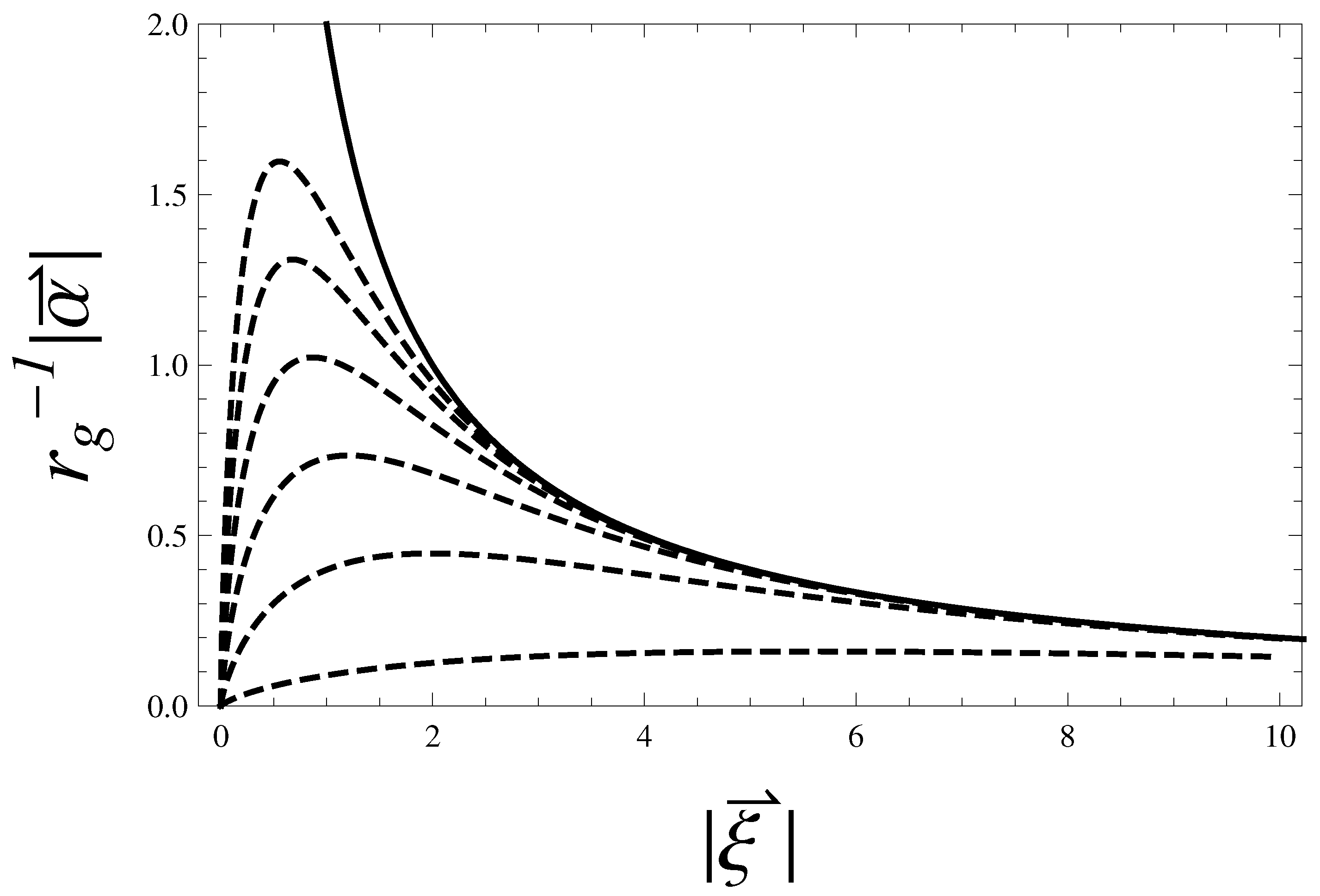
ξ the potential Φ outside the source is
Φ b a l l ( x ) = G M f X ( 0 ) | x | 1 + F ( μ 1 ξ ) 3 e μ 1 | x | 4 F ( μ 2 ξ ) 3 e μ 2 | x |
where F ( x ) = 3 x cosh x sinh x x 3 is a geometric factor depending on the form of source and satisfying the condition lim x 0 F ( x ) = 1 .
Besides the Birkhoff theorem results modified at Newtonian level: the solution can be only factorized by a space-depending function and an arbitrary time-depending function [56,76]. Furthermore the correction to the gravitational potential is depending on the only first two derivatives of f with rispect the X and the first derivatives with rispect the Y and Z in the point X = Y = Z = 0 . This means that different analytical theories, from the third derivative perturbation terms on, admit the same Newtonian limit [55,56,57].
For a right physical interpretation of Φ in Equation (38) we also impose the condition μ 1 4 μ 2 < 0 . This is a necessary condition for a correct interpretation of attractive gravitational potential, in addition to the condition μ 1 < μ 2 for a well with a negative minimum in | x | = 0 . These conditions can be summarized in terms of scale lengths. In fact we find that the contribution induced by Ricci and Riemann square goes to zero faster than the contribution induced by Ricci scalar: μ 1 1 > μ 2 1 . In terms of Lagrangian it means that for any f ( X , Y , Z ) -gravity the correction to Hilbert-Einstein Lagrangian depends more on the contributions of Ricci scalar ( f X X ( 0 ) 0 ) than ones of Ricci and Riemann square ( f Y ( 0 ) , f Z ( 0 ) 0 ). Then, if we suppose f X ( 0 ) > 0 (for a right Newtonian limit), starting from the condition μ 1 < μ 2 we get a constraint on the derivatives of f with respect to curvature invariants
f X X ( 0 ) + f Y ( 0 ) + 2 f Z ( 0 ) < 0
In the case of f ( R ) -gravity ( f Y ( 0 ) = f Z ( 0 ) = 0 ) we reobtain the same condition among the first and second derivatives of f [55,56,57,58].

3.2. f ( X , Y , Z ) -Gravity and the Quadratic Lagrangian

The outcome Equation (38) can be obtained also by considering the so-called Quadratic Lagrangian L = g ( a 1 R + a 2 R 2 + a 3 R α β R α β ) where a 1 , a 2 and a 3 are constants. In this case, [58] we find two characteristic lengths 2 ( 3 a 2 + a 3 ) a 1 1 / 2 , a 3 a 1 1 / 2 and the Newtonian limit of theory implies as solution Equation (38). We can state, then, the Newtonian limit of any f ( X , Y , Z ) -gravity can be reinterpreted by introducing the Quadratic Lagrangian and the coefficients have to satisfy the following relations
a 1 = f X ( 0 ) , a 2 = 1 2 f X X ( 0 ) f Z ( 0 ) , a 3 = f Y ( 0 ) + 4 f Z ( 0 )
A first considerations about Equation (44) is regarding the characteristic lengths induced by f ( X , Y , Z ) -gravity. The second length μ 2 1 is originated from the presence, in the Lagrangian, of Ricci and Riemann tensor square, but also a theory containing only Ricci tensor square could show the same outcome (it is successful replacing the coefficients a i of Quadratic Lagrangian or renaming the function f). Obviously the same is valid also with the Riemann tensor square alone. Then a such modification of theory enables a massive propagation of Ricci Tensor and, as it is well known in the literature, a substitution of Ricci Scalar with any function of Ricci scalar enables a massive propagation of Ricci scalar. We can, then, affirm that an hypothesis of Lagrangian containing any function of only Ricci scalar and Ricci tensor square is not restrictive and only the experimental constraints can fix the arbitrary parameters.
A second consideration is starting from the Gauss - Bonnet invariant defined by the relation G G B = X 2 4 Y + Z [77]. In fact the induced field equations satisfy in four dimensions the following condition
H μ ν G B = H μ ν X 2 4 H μ ν Y + H μ ν Z = 0
and by substituting them at Newtonian level ( H t t Z 4 R t t ( 2 ) ) in the Equation (19) we find the field equations (ever at Newtonian Level) of Quadratic Lagrangian which can be recasted as
f ( X , Y , Z ) = R 1 3 1 2 μ 1 2 + 1 μ 2 2 R 2 + R α β R α β μ 2 2
The theory of gravity represented by the Lagrangian Equation (46) is the more general theory considering all invariant curvatures, but we have to take into account a degeneracy. In fact we have different f ( X , Y , Z ) -gravity describing the same Newtonian Limit (see [55,56,57,58] for details). The solution of field equations or the observable quantities, as the galactic rotation curve, are parameterized by the derivatives of f, then we have different functions f ( X , Y , Z ) which admit the same physics in the weak field limit.

4. Stellar Hydrostatic Equilibrium in f ( R ) -Gravity

Extended Theories of Gravity could have important applications at stellar level. Here we outline how stellar structure equations result modified if the underlying theory of gravity is not GR.

4.1. The Newtonian Approach to the Hydrostatic Equilibrium

The condition of hydrostatic equilibrium for stellar structures in Newtonian dynamics is achieved by considering the equation [78]
d p d r = d Φ d r ρ
Together with the above equation, the Poisson equation
1 r 2 d d r r 2 d Φ d r = 4 π G ρ
gives the gravitational potential Φ as solution for a given matter density ρ. Since we are taking into account only static and stationary situations, here we consider only time-independent solutions (The radius r is assumed as the spatial coordinate. It ranges from r = 0 at the stellar center to r = ξ at the surface of the star). In general, the temperature τ appears in Equation (47) and Equation (48) the density satisfies an equation of state of the form ρ = ρ ( p , τ ) . In any case, we assume that there exists a polytropic relation between p and ρ of the form
p = K ρ γ
where K and γ are constant. The polytropic constant K is fixed and can be obtained as a combination of fundamental constants. However, there are several realistic cases where K is not fixed and another equation for its evolution is needed. The constant γ is the polytropic exponent. Inserting the polytropic equation of state into Equation (47), we obtain
d Φ d r = γ K ρ γ 2 d ρ d r
For γ 1 , the above equation can be integrated giving
γ K γ 1 ρ γ 1 = Φ ρ = γ 1 γ K 1 γ 1 ( Φ ) 1 γ 1 A n ( Φ ) n
where we have chosen the integration constant to give Φ = 0 at surface ( ρ = 0 ). The constant n is called the polytropic index and is defined as n = 1 γ 1 . Inserting the relation Equation (51) into the Poisson equation, we obtain a differential equation for the gravitational potential
d 2 Φ d r 2 + 2 r d Φ d r = 4 π G A n ( Φ ) n
Let us define now the dimensionless variables
z = | x | X A n ( Φ c ) n 1 2 w ( z ) = Φ Φ c = ( ρ ρ c ) 1 n
where the subscript c refers to the center of the star and the relation between ρ and Φ is given by Equation (51). At the center ( r = 0 ) , we have z = 0 , Φ = Φ c , ρ = ρ c and therefore w = 1 . Then Equation (52) can be written
d 2 w d z 2 + 2 z d w d z + w n = 0
This is the standard Lané-Embden equation describing the hydrostatic equilibrium of stellar structures in the Newtonian theory [78].

4.2. Hydrostatic Equilibrium in f ( R ) -Gravity

Let us consider now how hydrostatic equilibrium for stellar structures can change extending the theory to f ( R ) -gravity. In this case the action Equation (18) becomes
A = d 4 x g [ f ( R ) + X L m ]
The field equations are obtained by imposing f ( X , Y , Z ) f ( R ) in the Equation (19) and Equation (20). We get
f R μ ν f 2 g μ ν f ; μ ν + g μ ν f = X T μ ν 3 f + f R 2 f = X T
where f = f X . Since we are interested in analyzing the modification of Lané-Embden equation, it is sufficient to solve only the field equation for the gravitational potential Φ. In order to achieve the Newtonian limit of the theory, the metric tensor g μ ν Equation (21) can be approximated as follows
g μ ν 1 + 2 Φ ( x ) 0 0 δ i j
and the field Equation (26) become
R t t ( 2 ) R ( 2 ) 2 f ( 0 ) R ( 2 ) = X T t t ( 0 ) 3 f ( 0 ) R ( 2 ) R ( 2 ) = X T ( 0 )
where for the sake of simplicity we set f ( 0 ) = 1 . By the definition of mass Equation (40) and R t t ( 2 ) = Φ ( x ) we have
Φ R ( 2 ) 2 + R ( 2 ) 3 m 2 = X ρ ( m 2 ) R ( 2 ) = m 2 X ρ
We note that for f ( 0 ) 0 (or m ) we have the standard Poisson equation: Φ = 4 π G ρ . This means that as soon as the second derivative of f is different from zero, deviations from the Newtonian limit of GR emerge. The Equation (59) can be considered the modified Poisson equation for f ( R ) -gravity. They do not depend on gauge condition choice [58]. From the Bianchi identity, satisfied by the field Equation (19), we have
T μ ν ; μ = 0 p x k = 1 2 ( p + ρ ) ln g t t x k
If the dependence on the temperature τ is negligible, i.e., ρ = ρ ( p ) , this relation can be introduced into Equation (59), which become a system of three equations for p, Φ and R ( 2 ) and can be solved without the other structure equations.
Let us suppose that matter satisfies still a polytropic equation p = K ρ γ . If we introduce the relation Equation (51) into field Equation (59) we obtain an integro-differential equation for the gravitational potential Φ, that is
Φ ( x ) 2 X A n 3 ( Φ ( x ) ) n = m 2 X A n 6 d 3 x G m ( x , x ) ( Φ ( x ) ) n
The integro-differential nature of Equation (61) is the proof of the non-viability of Gauss theorem for f ( R ) -gravity. Adopting again the dimensionless variables
z = | x | ξ 0 , w ( z ) = Φ Φ c
where
ξ 0 3 2 X A n ( Φ c ) n 1
is a characteristic length linked to stellar radius ξ, Equation (61) becomes
d 2 w ( z ) d z 2 + 2 z d w ( z ) d z + w ( z ) n = m ξ 0 8 1 z 0 ξ / ξ 0 d z z e m ξ 0 | z z | e m ξ 0 | z + z | w ( z ) n
which is the modified Lané-Emden equation deduced from f ( R ) -gravity. Clearly the particular f ( R ) -model is specified by the parameters m and ξ 0 . If m (i.e., f ( R ) R ), Equation (64) becomes Equation (54). We are only interested in solutions of Equation (64) that are finite at the center, that is for z = 0 . Since the center must be an equilibrium point, the gravitational acceleration | g | = d Φ / d r d w / d z must vanish for w ( 0 ) = 0 . Let us assume we have solutions w ( z ) of Equation (64) that fulfill the boundary conditions w ( 0 ) = 1 and w ( ξ / ξ 0 ) = 0 ; then according to the choice Equation (62), the radial distribution of density is given by
ρ ( | x | ) = ρ c w n , ρ c = A n Φ c n
and the pressure by
p ( | x | ) = p c w n + 1 , p c = K ρ c γ
For γ = 1 (or n = ) the integro-differential Equation (64) is not correct. This means that the theory does not contain the case of isothermal sphere of ideal gas. In this case, the polytropic relation is p = K ρ . Putting this relation into Equation (60) we have
Φ K = ln ρ ln ρ c ρ = ρ c e Φ / K
where the constant of integration is chosen in such a way that the gravitational potential is zero at the center. If we introduce Equation (67) into Equation (59), we have
Φ ( x ) 2 X ρ c 3 e Φ ( x ) / K = m 2 X ρ c 6 d 3 x G m ( x , x ) e Φ ( x ) / K
Assuming the dimensionless variables z = | x | ξ 1 and w ( z ) = Φ K where ξ 1 3 K 2 X ρ c , Equation (68) becomes
d 2 w ( z ) d z 2 + 2 z d w ( z ) d z + e w ( z ) = m ξ 1 8 1 z 0 ξ / ξ 1 d z z e m ξ 1 | z z | e m ξ 1 | z + z | e w ( z )
which is the modified “isothermal” Lané-Emden equation derived f ( R ) -gravity.

4.3. Solutions for the Standard and Modified Lané-Emden Equations

The task is now to solve the modified Lané-Emden equation and compare its solutions to those of standard Newtonian theory. Only for three values of n, the solutions of Equation (54) have analytical expressions [78]
n = 0 w G R ( 0 ) ( z ) = 1 z 2 6 n = 1 w G R ( 1 ) ( z ) = sin z z n = 5 w G R ( 5 ) ( z ) = 1 1 + z 2 3
We label these solution with G R since they agree with the Newtonian limit of GR. The surface of the polytrope of index n is defined by the value z = z ( n ) , where ρ = 0 and thus w = 0 . For n = 0 and n = 1 the surface is reached for a finite value of z ( n ) . The case n = 5 yields a model of infinite radius. It can be shown that for n < 5 the radius of polytropic models is finite; for n > 5 they have infinite radius. From Equation (70) one finds z G R ( 0 ) = 6 , z G R ( 1 ) = π and z G R ( 5 ) = . A general property of the solutions is that z ( n ) grows monotonically with the polytropic index n. In Figure 1 we show the behavior of solutions w G R ( n ) for n = 0 , 1 , 5 . Apart from the three cases where analytic solutions are known, the classical Lané-Emden Equation (54) has to be be solved numerically, considering with the expression
w G R ( n ) ( z ) = i = 0 a i ( n ) z i
for the neighborhood of the center. Inserting Equation (71) into Equation (54) and by comparing coefficients one finds, at lowest orders, a classification of solutions by the index n, that is
w G R ( n ) ( z ) = 1 z 2 6 + n 120 z 4 +
Figure 1. Plot of solutions (blue lines) of standard Lané-Emden Equation (54): w G R ( 0 ) ( z ) (dotted line) and w G R ( 1 ) ( z ) (dashed line). The green line corresponds to w G R ( 5 ) ( z ) . The red lines are the solutions of modified Lané-Emden Equation (64): w f ( R ) ( 0 ) ( z ) (dotted line) and w f ( R ) ( 1 ) ( z ) (dashed line). The blue dashed-dotted line is the potential derived from GR ( w G R ( z ) ) and the red dashed-dotted line the potential derived from f ( R ) -gravity ( w f ( R ) ( z ) ) for a uniform spherically symmetric mass distribution. The assumed values are m ξ = 1 and m ξ 0 = 0 . 4 . From a rapid inspection of these plots, the differences between GR and f ( R ) gravitational potentials are clear and the tendency is that at larger radius z they become more evident.
Galaxies 02 00520 g001
The case γ = 5 / 3 and n = 3 / 2 is the non-relativistic limit while the case γ = 4 / 3 and n = 3 is the relativistic limit of a completely degenerate gas.
Also for modified Lané-Emden Equation (64), we have an exact solution for n = 0 . In fact, it is straightforward to find out
w f ( R ) ( 0 ) ( z ) = 1 z 2 8 + ( 1 + m ξ ) e m ξ 4 m 2 ξ 0 2 1 sinh m ξ 0 z m ξ 0 z
where the boundary conditions w ( 0 ) = 1 and w ( 0 ) = 0 are satisfied. A comment on the GR limit (that is f ( R ) R ) of solution Equation (73) is necessary. In fact when we perform the limit m , we do not recover exactly w G R ( 0 ) ( z ) . The difference is in the definition of quantity ξ 0 . In f ( R ) -gravity we have the definition Equation (63) while in GR it is ξ 0 = 2 X A n Φ c n 1 , since in the first equation of Equation (59), when we perform f ( R ) R , we have to eliminate the trace equation condition. In general, this means that the Newtonian limit and the Eddington parameterization of different relativistic theories of gravity cannot coincide with those of GR (see [16] for further details on this point).
The point z f ( R ) ( 0 ) is calculated by imposing w f ( R ) ( 0 ) ( z f ( R ) ( 0 ) ) = 0 and by considering the Taylor expansion
sinh m ξ 0 z m ξ 0 z 1 + 1 6 ( m ξ 0 z ) 2 + O ( m ξ 0 z ) 4
we obtain z f ( R ) ( 0 ) = 2 6 3 + ( 1 + m ξ ) e m ξ . Since the stellar radius ξ is given by definition ξ = ξ 0 z f ( R ) ( 0 ) , we obtain the constraint
ξ = 3 Φ c 2 π G 1 1 + 1 + m ξ 3 e m ξ
By solving numerically the constraint (In principle, there is a solution for any value of m) Equation (75), we find the modified expression of the radius ξ. If m we have the standard expression ξ = 3 Φ c 2 π G valid for the Newtonian limit of GR. Besides, it is worth noticing that in the f ( R ) -gravity case, for n = 0 , the radius is smaller than in GR. On the other hand, the gravitational potential Φ gives rise to a deeper potential well than the corresponding Newtonian potential derived from GR [58].
In the case n = 1 , Equation (64) can be recast as follows
d 2 w ˜ ( z ) d z 2 + w ˜ ( z ) = m ξ 0 8 0 ξ / ξ 0 d z e m ξ 0 | z z | e m ξ 0 | z + z | w ˜ ( z )
where w ˜ = z w . If we consider the solution of Equation (76) as a small perturbation to the one of GR, we have
w ˜ f ( R ) ( 1 ) ( z ) w ˜ G R ( 1 ) ( z ) + e m ξ Δ w ˜ f ( R ) ( 1 ) ( z )
The coefficient e m ξ < 1 is the parameter with respect to which we perturb Equation (76). Besides these position ensure us that when m the solution converge to something like w ˜ G R ( 1 ) ( z ) . Substituting Equation (77) in Equation (76), we have
d 2 Δ w ˜ f ( R ) ( 1 ) ( z ) d z 2 + Δ w ˜ f ( R ) ( 1 ) ( z ) = m ξ 0 e m ξ 8 0 ξ / ξ 0 d z e m ξ 0 | z z | e m ξ 0 | z + z | w ˜ G R ( 1 ) ( z )
and the solution is easily found
w f ( R ) ( 1 ) ( z ) sin z z 1 + m 2 ξ 0 2 8 ( 1 + m 2 ξ 0 2 ) 1 + 2 e m ξ 1 + m 2 ξ 0 2 ( cos ξ / ξ 0 + m ξ 0 sin ξ / ξ 0 ) m 2 ξ 0 2 8 ( 1 + m 2 ξ 0 2 ) 2 e m ξ 1 + m 2 ξ 0 2 ( cos ξ / ξ 0 + m ξ 0 sin ξ / ξ 0 ) sinh m ξ 0 z m ξ 0 z + cos z
Also in this case, for m , we do not recover exactly w G R ( 1 ) ( z ) . The reason is the same of previous n = 0 case [16]. Analytical solutions for other values of n are not available.
To conclude this section, we report the gravitational potential profile generated by a spherically symmetric source of uniform mass with radius ξ. By solving field Equation (59) inside the star and considering the boundary conditions w ( 0 ) = 1 and w ( 0 ) = 0 , we get
w f ( R ) ( z ) = 3 2 ξ + 1 m 2 ξ 3 e m ξ ( 1 + m ξ ) m 2 ξ 3 1 3 2 ξ + 1 m 2 ξ 3 ξ 0 2 z 2 2 ξ 3 e m ξ ( 1 + m ξ ) m 2 ξ 3 sinh m ξ 0 z m ξ 0 z
In the limit m , we recover the GR case w G R ( z ) = 1 ξ 0 2 z 2 3 ξ 2 . In Figure 1 we show the behaviors of w f ( R ) ( 0 ) ( z ) and w f ( R ) ( 1 ) ( z ) with respect to the corresponding GR cases. Furthermore, we plot the potential generated by a uniform spherically symmetric mass distribution in GR and f ( R ) -gravity and thecase w G R ( 5 ) ( z ) .
An important remark is in order at this point. In a general discussion of the problem, also time-dependent perturbations should be taken into account. In particular, quadratic gravity possess gosth-like instability related to the sign of coefficient in front of the term R 2 . In such cases, unstable or unphysical solutions come out and have to be discriminated with respect to physical cases. A discussion in this sense is in [38,39].

5. Rotation Curves of Galaxies

Another important astrophysical application of the above Newtonian limit of Fourth Order Gravity is related to the rotation curves of spiral galaxies. The approach can be considered also an alternative test for DM behavior.
In general, the motion of body embedded in the gravitational field is given by geodesic Equation (5) and in the Newtonian limit, formally, we obtain the classical structure of the motion Equation (7)
d 2 x d t 2 = Φ ( x )
but the gravitational potential is given by Equation (38) or generally by Equation (41). The study of motion is very simple if we consider a particular symmetry of mass distribution ρ, otherwise the analytical solutions are not available. Our aim is to evaluate the corrections to the classical motion in the easiest situation: the circular motion. In this case we do not consider the radial and vertical motion. The condition of stationary motion on the circular orbit is
v c ( | x | ) 2 | x | = Φ ( x ) | x |
where v c is the velocity.
The distribution of mass can be modeled simply by introducing two sets of coordinates: the spherical coordinates ( r , θ , ϕ ) and the cylindrical coordinates ( R , θ , z ) . An useful mathematical tool is the Gauss flux theorem for gravity: The gravitational flux through any closed surface is proportional to the enclosed mass. The law is expressed in terms of the gravitational field. The gravitational field g is defined so that the gravitational force experienced by a particle with mass m is F g r a v = m g . Since the Newtonian mechanics satisfies this theorem and, by thinking to a spherical system of mass distribution, we get, from Equation (82), the equation
v c ( r ) 2 = G M ( r ) r = 4 π G r 0 r d y y 2 ρ ( y )
where M ( r ) is the only mass enclosed in the sphere with radius r. The Green function of the f ( X , Y , Z ) -gravity ( | x x | 1 ), instead, does not satisfy the theorem [58]. In this case we must consider directly the gravitational potential Equation (41) generated by using the superposition principle.
Apart the mathematical difficulties incoming from the research of gravitational potential for a given mass distribution, the non-validity of Gauss theorem implies, for example, that a sphere can not be reduced to a point (see solution Equation (42)). In fact the gravitational potential generated by a ball (also with constant density) is depending also on the Fourier transform of ball [58]. However, our aim is to consider not the simple case of motion of body in the vacuum, but the more interesting case of motion in the matter. So we must leave any possibility of idealization and consider directly the calculation of the potential Equation (41).
Two remarks on the Equation (41) are needed. The two corrections have different algebraic sign, and in particular the Yukawa correction with μ 1 implies a stronger gravitational force, while the second one (purely induced by Ricci and Riemann square) contributes with a repulsive force. By remembering that the motivations of extending the outcome of GR to new theories is supported by missing matter justifying the flat rotation curves of galaxies, the first correction is a nice candidate. A crucial point is given by the spatial range of correction. In fact the Yukawa corrections imply a massive propagation; then, more massive is the particle, shorter is the spatial range.
At last in Newtonian Mechanics the Gauss theorem gives us a spherically symmetric gravitational potential even if the spherically symmetric source is rotating. In GR as well as in Fourth Order Gravity, however, the rotating spherically symmetric source generates an axially symmetric space-time (the well known Kerr metric) and only if the source is at rest one has the space-time with the same symmetry (the well known Schwarzschild metric). Then the galaxy being a rotating system will generate an axially symmetric space-time while we are using the solution Equation (41). This aspect is not contradictory because the solutions are calculated in the Newtonian limit (i.e., v 2 1 ) and under this assumption the Kerr metric collapses into Schwarzschild metric. In fact we have
g μ ν K e r r = 1 r g r Σ 2 0 0 r g r η Σ 2 sin 2 θ 0 Σ 2 H 2 0 0 0 0 Σ 2 0 r g r η Σ 2 sin 2 θ 0 0 r 2 + η 2 + r g r η 2 Σ 2 sin 2 θ sin 2 θ g μ ν S c h w = 1 r g r 0 0 0 0 1 r g r 0 0 0 0 r 2 0 0 0 0 r 2 sin 2 θ
where Σ 2 = r 2 + η 2 cos 2 θ , H 2 = r 2 r g r + η 2 , η = L / M and L is the angular momentum along the z-axis.

5.1. Mass Models for Galaxies

From the point of view of morphology, a galaxy can be modeled by considering at least two components: the bulge and the disk. Obviously the galaxy is a more complicated structure and there are others components, but for our aim this idealization is satisfactory. The bulge, generally, can be represented easily with cylindrical coordinates (but in a more crude idealization it is like a ball), while the disk has a radius bigger than the thickness. However, we find that the rotation curve does not present the Keplerian behavior outside the matter, but the curve remain constant for any distance. Then we must formulate the existence of exotic matter that can justify the experimental observation. A simple discussion about the distribution of DM can be formulated by imposing the constant value of velocity in Equation (83) for large distances. In fact we find
v c ( r ) constant ρ D M ( r ) r 2
A matter distribution as Equation (85) has a problem when we want to calculate the total mass. In fact if we have ρ r 2 , the mass diverges. A such exotic behavior seems no-physical, but this outcome is only the consequence of constant rotation curve. In fact by increasing the distance also the mass must increase with the power law for any distance Equation (83). However, since the Gauss theorem holds in GR, the matter outside the sphere of integration does not contribute to the gravitational flux and then we do not have difference with respect to the ordinary matter.
The same arguments are not valid in f ( X , Y , Z ) -gravity: the non-viability of Gauss theorem implies that the range of integration of DM could cover all range and also the matter outside is considered. A cut off is needed now. Here then, for completeness, we consider that the galaxy is composed by three components: the bulge, the disk and an alone of DM.
It should be noted that the spatial behaviors of DM (generally spherically symmetric) are made only a posteriori: the cornerstones of rotation curves study are the GR and the distribution of ordinary matter. Only after this assumption the distribution of DM is such as to justify the gap between the theoretical prediction and the experimental observation.
Before jumping to analysis of rotation curves we want to resume the principal spatial distributions of mass in the three galactic components. In literature there are many forms of density, but it is possible to resume them as follows.
More realistic models are the ones with mass density depending also on the z-coordinate for bulge and disk. Particularly one can consider the following choice
ρ b u l g e ( R , z ) = M b 4 π V 0 ξ b γ [ R 2 + z 2 / q 2 ] γ / 2 ξ b + R 2 + z 2 / q 2 ξ b γ β e R 2 + z 2 / q 2 ξ t 2 ρ d i s k ( R , z ) = M d 4 π ξ d 2 z d e R ξ d | z | z d ρ D M ( r ) = M D M v i r 4 π ξ s 3 g ( ξ D M v i r / ξ s ) ξ s r 1 [ 1 + r / ξ s ] 2
In this choice, suggested by Dehnen & Binney [80], the bulge is described as a truncated power—law model (first line of Equation (86)) where V 0 = 0 d R R 0 d z ρ ˜ b u l g e ( R , z ) . β, γ, q and ξ t are the parameters. While for the disk, one adopted a double exponential where the total mass is M d = 2 π ξ d 2 Σ e ξ 0 ξ d with Σ = ( 48 ± 8 ) M / pc 2 and ξ 0 = 8 . 5 Kpc [81]. Finally in the case of DM the density profile is the Navarro-Frenk-White model [7,82] where g ( x ) = ln ( 1 + x ) x x + 1 , M D M v i r and ξ D M v i r are the virial mass and virial radius and ξ s is a characteristic length. For the Milky Way ξ D M v i r / ξ s = 10 ÷ 15 .
Leaving the axis-symmetry one can consider a more simple model: the spherical symmetry model. With this approach one has [83,84,85]
ρ b u l g e ( r ) = k M b 4 η π ξ b 9 / 4 r d x e k [ ( x / ξ b ) 1 / 4 1 ] x 3 / 4 x 2 r 2 σ d i s k ( R ) = M d 2 π ξ d 2 e R ξ d ρ D M ( r ) = M D M 2 ( 4 π ) π ξ D M 3 1 1 + r 2 ξ D M 2
where ξ b , ξ d , ξ D M , M b , M d , M D M , are the radii and the masses of bulge, disk and DM. k = 7 . 6695 and η = 22 . 665 are dimensionless constants. The density profile of bulge considered is the well-known formula of de Vaucouleurs [86].
A simpler model, resuming the previous ones, can be
ρ b u l g e ( r ) = M b 2 π ξ b 3 γ Γ ( 3 γ 2 ) e r 2 ξ b 2 r γ σ d i s k ( R ) = M d 2 π ξ d 2 e R ξ d ρ D M ( r ) = α M D M π ( 4 π ) ξ D M 3 1 1 + r 2 ξ D M 2
where Γ ( x ) is the Gamma function, 0 γ < 3 is a free parameter and 0 α < 1 is the ratio of DM inside the sphere with radius ξ D M with respect to the total DM. The radius ξ D M and the mass M D M play conceptually the same role respectively of ξ D M v i r and M D M v i r . However, as before claimed, the hot point is the choice of DM model. Given all these models it is almost normal that there are many different estimates of DM. Therefore, the parameters of DM model may not be unique [87].

5.2. Rotation Curves in f ( X , Y , Z ) -Gravity

We are interested to evaluate the circular velocity Equation (82) adopting the mass models Equation (88). So the potential Equation (41), by setting f X ( 0 ) = 1 , becomes
Φ ( r , R , z ) = G { 2 M b 3 ξ b 3 γ Γ ( 3 γ 2 ) 1 r 0 d r r 1 γ e r 2 ξ b 2 [ 3 | r r | r r 2 e μ 1 a | r r | e μ 1 a ( r + r ) 2 μ 1 a + 2 e μ 2 a | r r | e μ 2 a ( r + r ) μ 2 a ] + 4 α M D M 3 ( 4 π ) ξ D M 3 1 r 0 Ξ / a d r r 1 + r 2 ξ D M 2 [ 3 | r r | r r 2 e μ 1 a | r r | e μ 1 a ( r + r ) 2 μ 1 a + 2 e μ 2 a | r r | e μ 2 a ( r + r ) μ 2 a ] M d π ξ d 2 [ 0 d R e R ξ d R K ( 4 R R ( R + R ) 2 + z 2 ) ( R + R ) 2 + z 2 + K ( 4 R R ( R R ) 2 + z 2 ) ( R R ) 2 + z 2 + 0 d R e R ξ d R 0 π d θ e μ 1 a Δ ( R , R , z , 0 , θ ) 4 e μ 2 a Δ ( R , R , z , 0 , θ ) 3 Δ ( R , R , z , 0 , θ ) ] }
where Ξ is the distance on which we observe the rotation curve, K is the elliptic function and the modulus of distance is given by
Δ ( R , R , z , z , θ ) | x x | = ( R + R ) 2 + ( z z ) 2 4 R R cos 2 θ
The constant a is a scale factor defined by the substitution R , r a r , a R so all quantities are dimensionless. At last, by remembering r = R 2 + z 2 the circular speed Equation (82) in the galactic plan is given by
v c ( R ) = R R Φ ( R , R , 0 )
In the Figure 2 and Figure 3, we report the spatial behaviors of rotation curve induced by the bulge and disk component. The behavior for any component is compared in the framework of GR, Fourth Order Gravity (FOG), GR + DM and FOG + DM. The values of free parameters of model are in the first line in Table 1 and refereing to Milky Way. The values of scale lengths μ 1 , μ 2 are set at 10 2 a 1 , 10 2 a 1 . In both components we note for R > > ξ b , ξ d the Keplerian behavior, while it is missing only when we consider also the DM component. The shape of the rotation curve is similar to ones obtained by varying the total mass and scale radius. For a given scale radius, the peak velocity varies proportionally to a square root of the mass. For a fixed total mass, the peak-velocity position moves inversely proportionally to the scale radius, or along a Keplerian line.
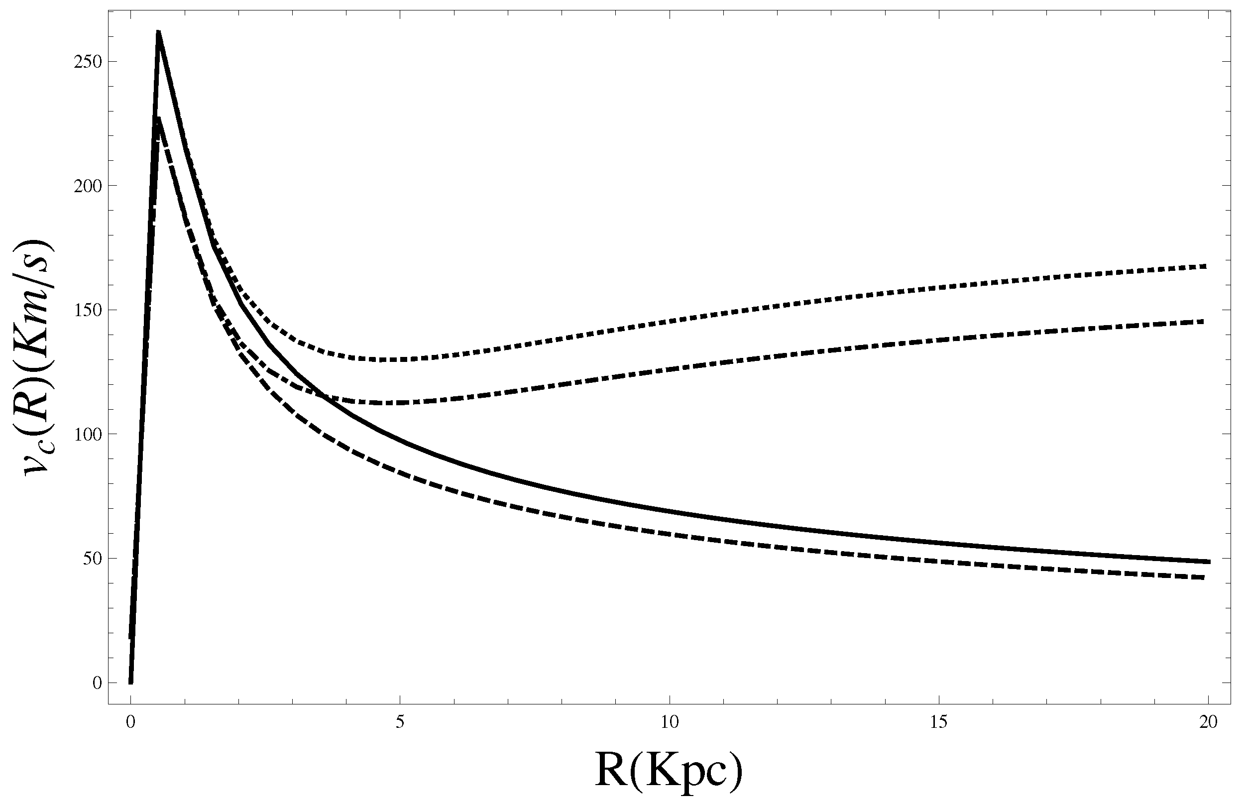
Figure 2. The rotation curve induced by bulge component (first line of Equation (88)): GR (dashed line), GR + DM (dashed and dotted line), FOG (solid line) and FOG + DM (dotted line).
Galaxies 02 00520 g002
As it is known in literature f ( X , Y , Z ) -gravity, and in particular f ( R ) -gravity, mimics a partial contribution of DM. In fact the corrective term e μ 1 | x | / | x | contributes to enhance the attraction and thus the rotation curve must increase to balance the force. In the case of the other term, we have a correction e μ 2 | x | / | x | that contributes, being repulsive, to decrease the velocity. However, in both cases these terms are asymptotically null and f ( X , Y , Z ) -gravity and GR must lead to the same result. Only with the addition of DM it is possible to raise the curve and have almost constant values. In the Figure 4 we report the component of rotation curve induced by only auto-gravitating DM.
Figure 3. The rotation curve induced by disk component (second line of Equation (88)): GR (dashed line), GR + DM (dashed and dotted line), FOG (solid line) and FOG + DM (dotted line).
Galaxies 02 00520 g003
Table 1. Parameters of models Equation Equation (88). The unity of mass is 10 10 M and a = 1 Kpc .
Galaxy M b ξ b γ M d ξ d M DM ξ DM αΞ
Milky Way0.770.51.55.203.51.685.50.5020
NGC 31980//2.603.50.845.50.5320
Figure 4. The rotation curve induced by DM component (third line of Equation (88)): GR + DM (dashed and dotted line) and FOG + DM (dotted line).
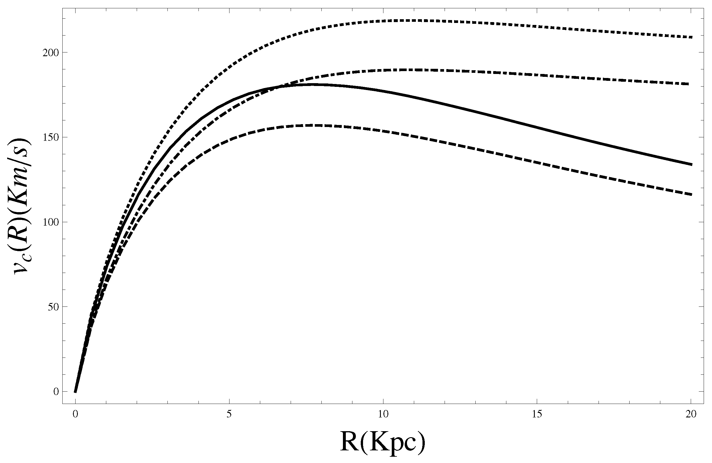
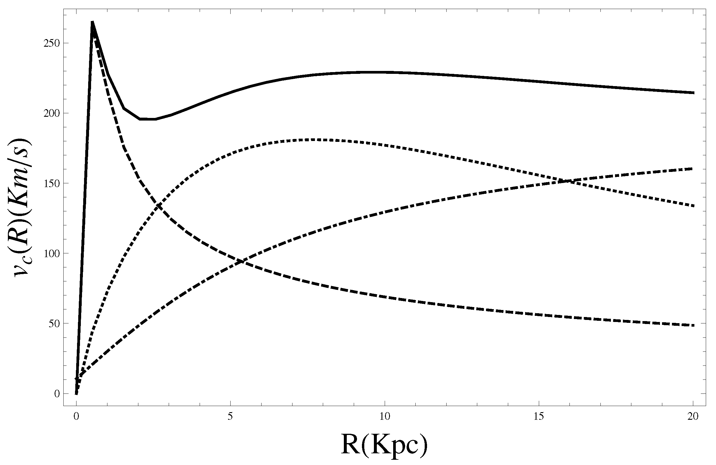
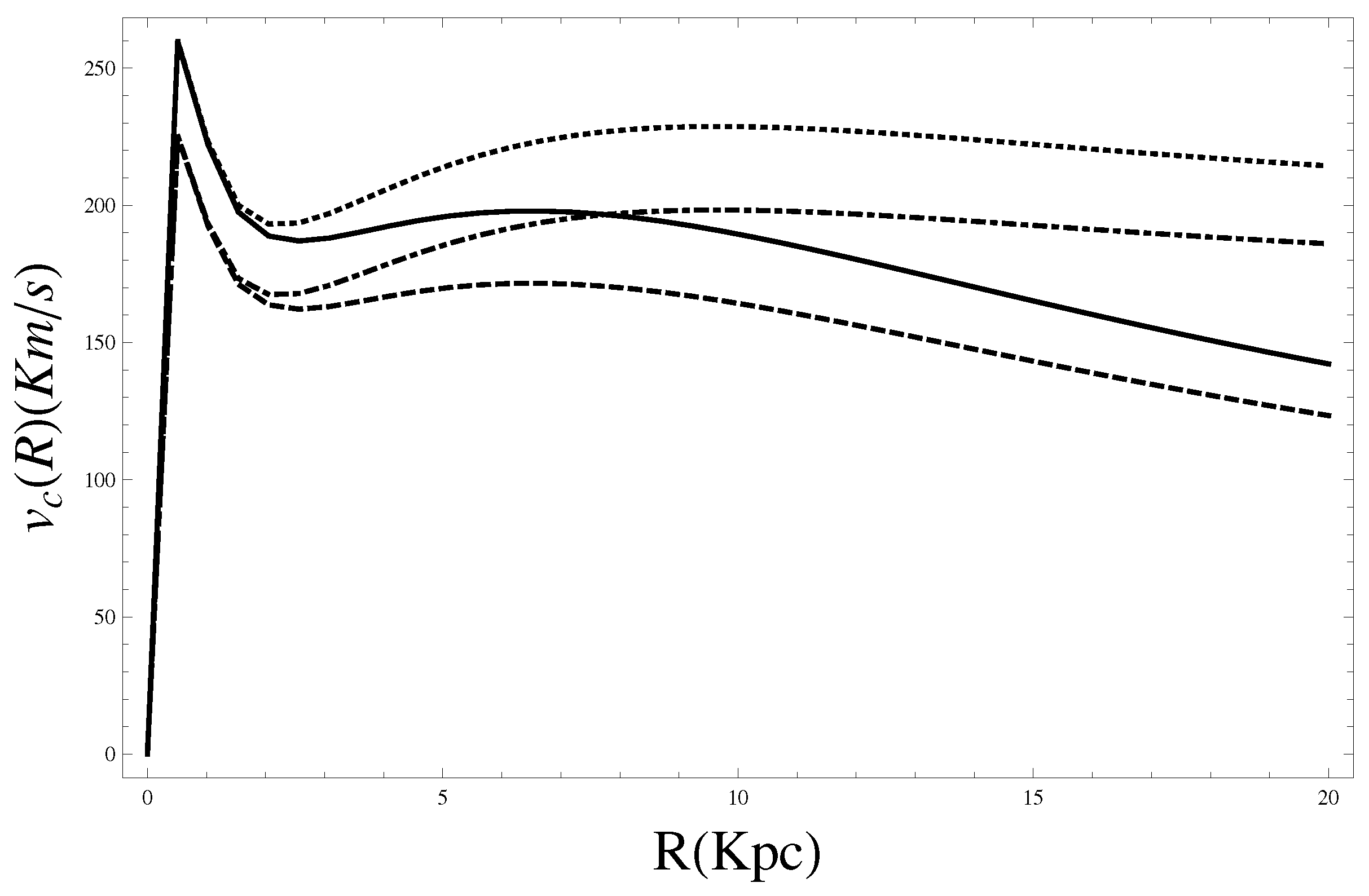
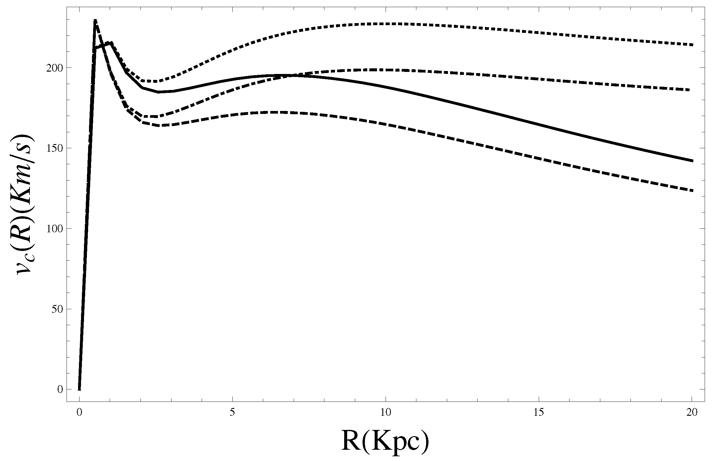
Galaxies 02 00520 g004
In Figure 5 we show the global behavior (experimentally expected) of rotation curve compared with respect to the bulge, disk and DM component for the f ( X , Y , Z ) -gravity. While in Figure 6 there is the global rotation curve in the framework of GR, FOG, GR + DM and FOG + DM. At last in Figure 7 we replicate the outcome of Figure 6 but we inserted the value μ 2 = 5 a 1 . In this case the rotation curve induced by f ( X , Y , Z ) -gravity allows lower values as previously we claimed.
Figure 5. Comparison between the rotation curves of galactic components: bulge (dashed line), disk (dotted line), DM (dotted and dashed line) and the global galactic rotation curve (solid line). All curves have been valuated in the framework of FOG + DM.
Galaxies 02 00520 g005
Figure 6. The global rotation curve in the framework of GR (dashed line), GR + DM (dashed and dotted line), FOG (solid line) and FOG + DM (dotted line). The values of “masses” are μ 1 = 10 2 a 1 and μ 2 = 10 2 a 1 .
Galaxies 02 00520 g006
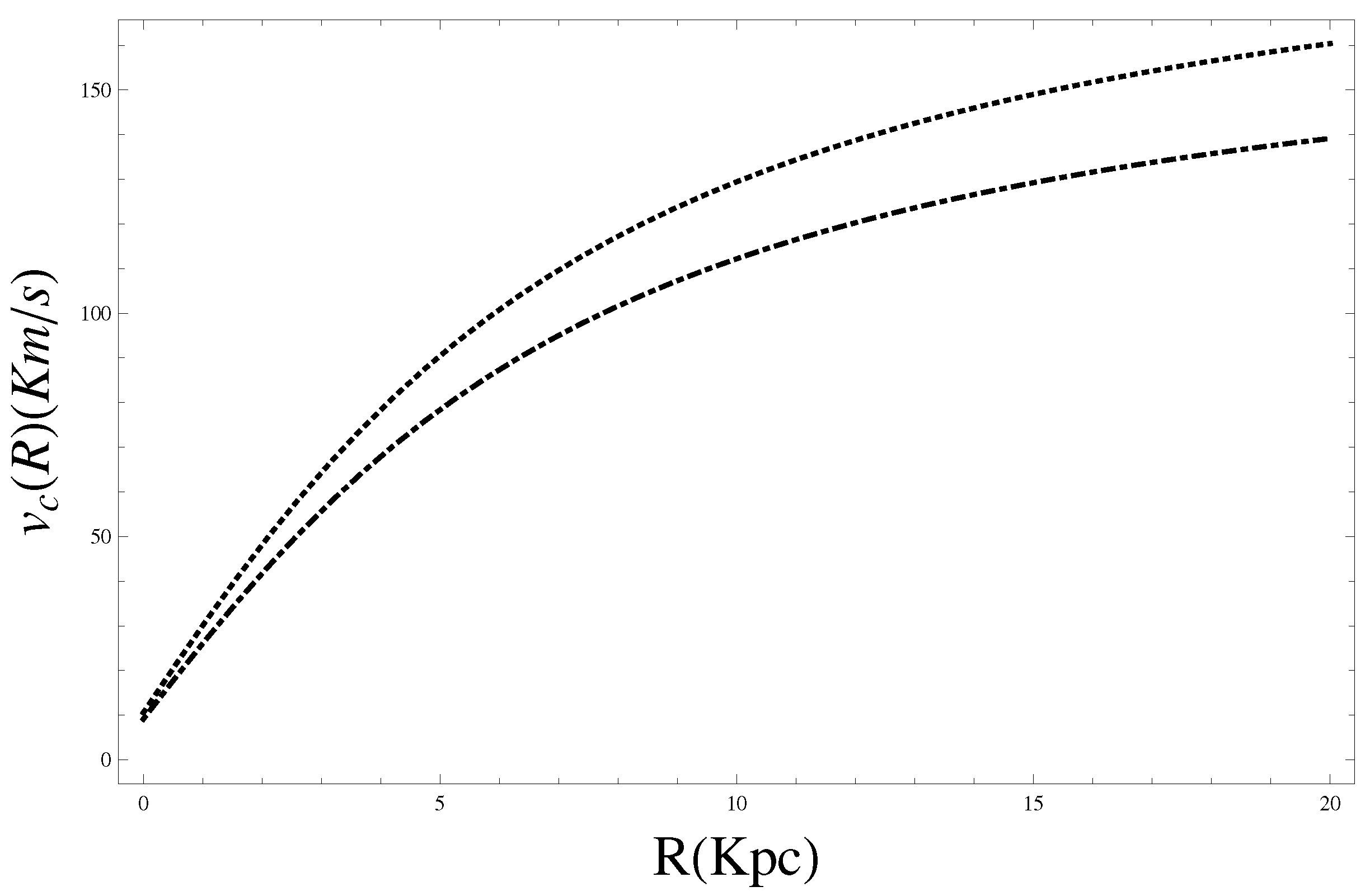
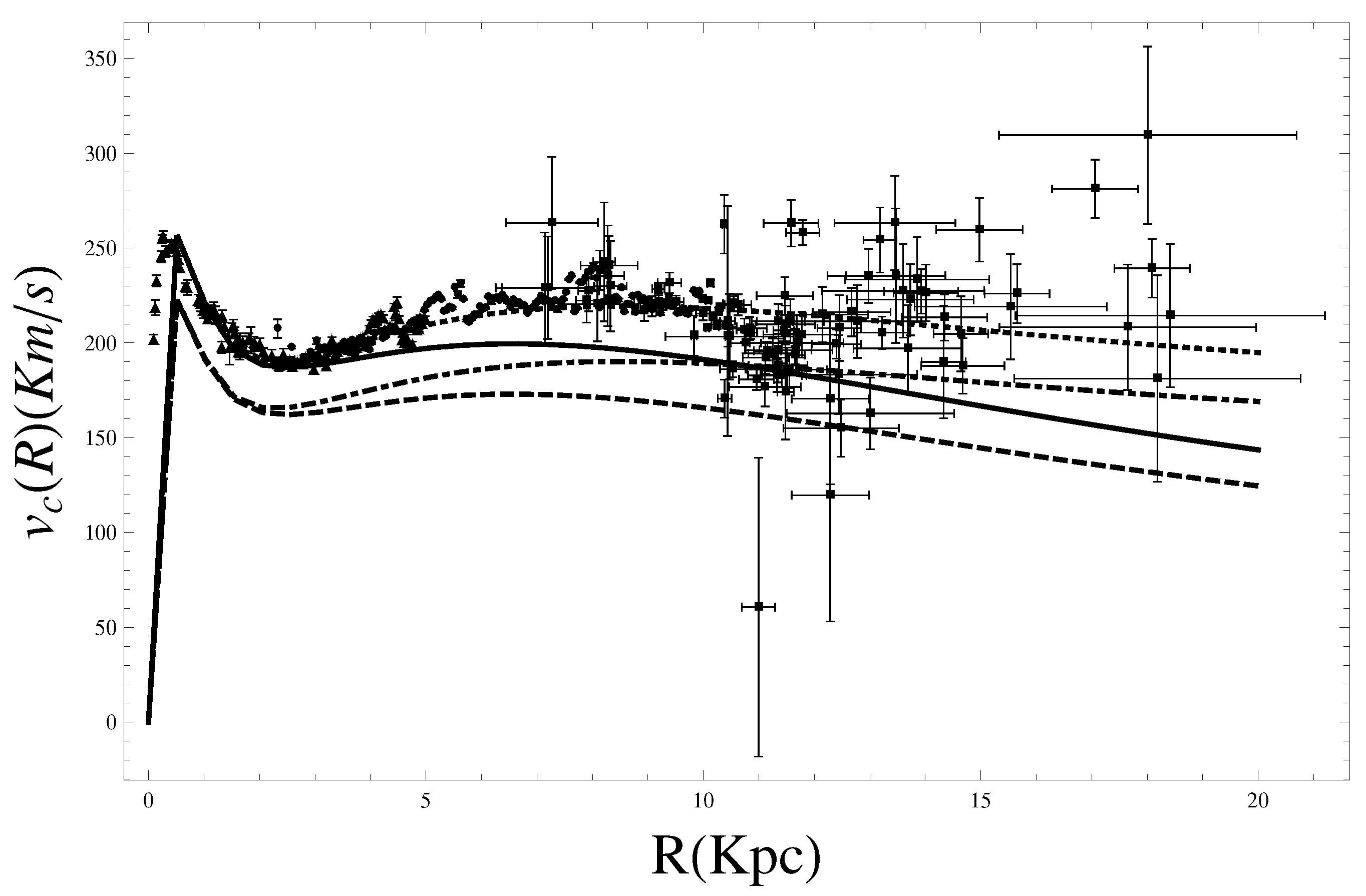
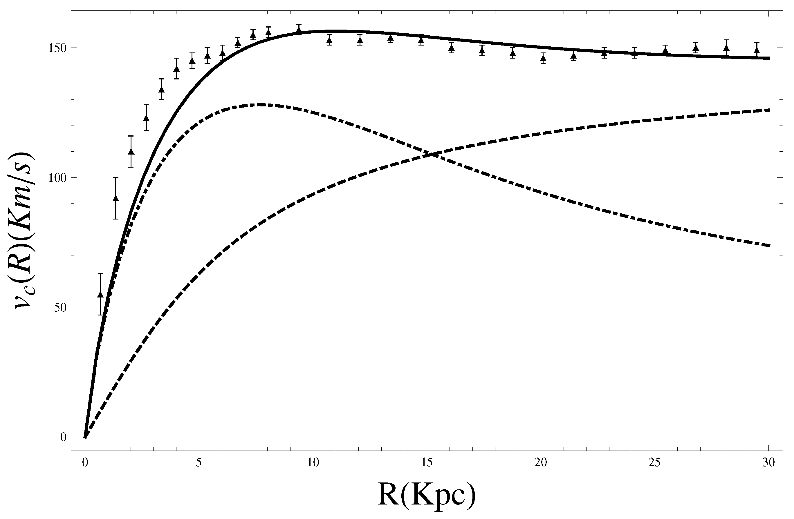
From the experimental point of view we used an updated rotation curve of Milky Way by integrating the existing data from the literature, and plot them in the same scale [88]. The data used are available in a digitized [89]. The unified rotation curve shows clearly the three dominant components: bulge, disk, and flat rotation due to the DM [90,91,92,93,94,95,96,97]. These data, finally, have been updated further by [98]. The whole set of data are plotted in Figure 8 and on them the theoretical rotation curve induced by f ( X , Y , Z ) -gravity with DM has been superimposed. The values of best fit are shown in Table 1 with μ 1 = 10 2 Kpc 1 and μ 2 = 10 2 Kpc 1 .
Figure 7. The global rotation curve in the framework of GR (dashed line), GR + DM (dashed and dotted line), FOG (solid line) and FOG + DM (dotted line). The values of “masses” are μ 1 = 10 2 a 1 and μ 2 = 5 a 1 .
Galaxies 02 00520 g007
Figure 8. Superposition of theoretical behaviors (GR (dashed line), GR + DM (dashed and dotted line), FOG (solid line), FOG + DM (dotted line)) on the experimental data for Milky Way. The mass model used is shown in Equation (88) and the values of parameters are in Table 1. The values of “masses” are μ 1 = 10 2 Kpc 1 and μ 2 = 10 2 Kpc 1 .
Galaxies 02 00520 g008
The same mass model Equation (88) has been considered also for the galaxy NGC 3198. This galaxy has been chosen since the bulge is missing. Then we set M b = 0 in the Equation (89). In Figure 9 we show the experimental data [99] and the superposition of theoretical behavior. Also in this case we find a nice outcome for a new set of parameters shown in Table 1, while the values of μ 1 and μ 2 are the same of Milky Way.
The initial aim, i.e., to extend the GR to a new class of theories, as we claimed in the introduction, is to justify the rotation curve without the DM component. From the previous outcomes, we see that even if the f ( X , Y , Z ) -gravity, or better a f ( R ) -gravity, admits a stronger attractive force, it is unable to realize our aim. Also in this framework we need Dark Matter. Obviously we need a smaller amount of DM on the middle distances, but for large distances we have the same problems of GR.
Figure 9. Superposition of theoretical behaviors (GR (dashed line), GR + DM (dashed and dotted line), FOG (solid line), FOG + DM (dotted line)) on the experimental data for NGC 3198. The mass model used is shown in Equation (88) and the values of parameters are in Table 1. The values of “masses” are μ 1 = 10 2 Kpc 1 and μ 2 = 10 2 Kpc 1 .
Galaxies 02 00520 g009

5.3. Rotation Curves in R N -Gravity and f ( X , Y , Z ) -Gravity

The problem of DM seems to have been solved in literature, in the framework of f ( R ) -
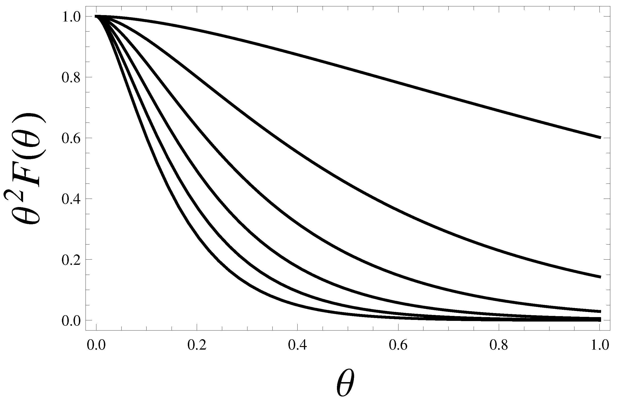
gravity, by considering the Lagrangian L = R n with n ϵ Q [59,62]. In these papers the gravitational potential for a point-like source can be
Φ R n ( r ) = G M r 1 + ( r / r c ) β 1 2
where r c is a characteristic length and β is a dimensionless parameter. To recover the condition lim r Φ R n ( r ) = 0 one must have 0 β < 1 . In the case β = 0 the GR is found.
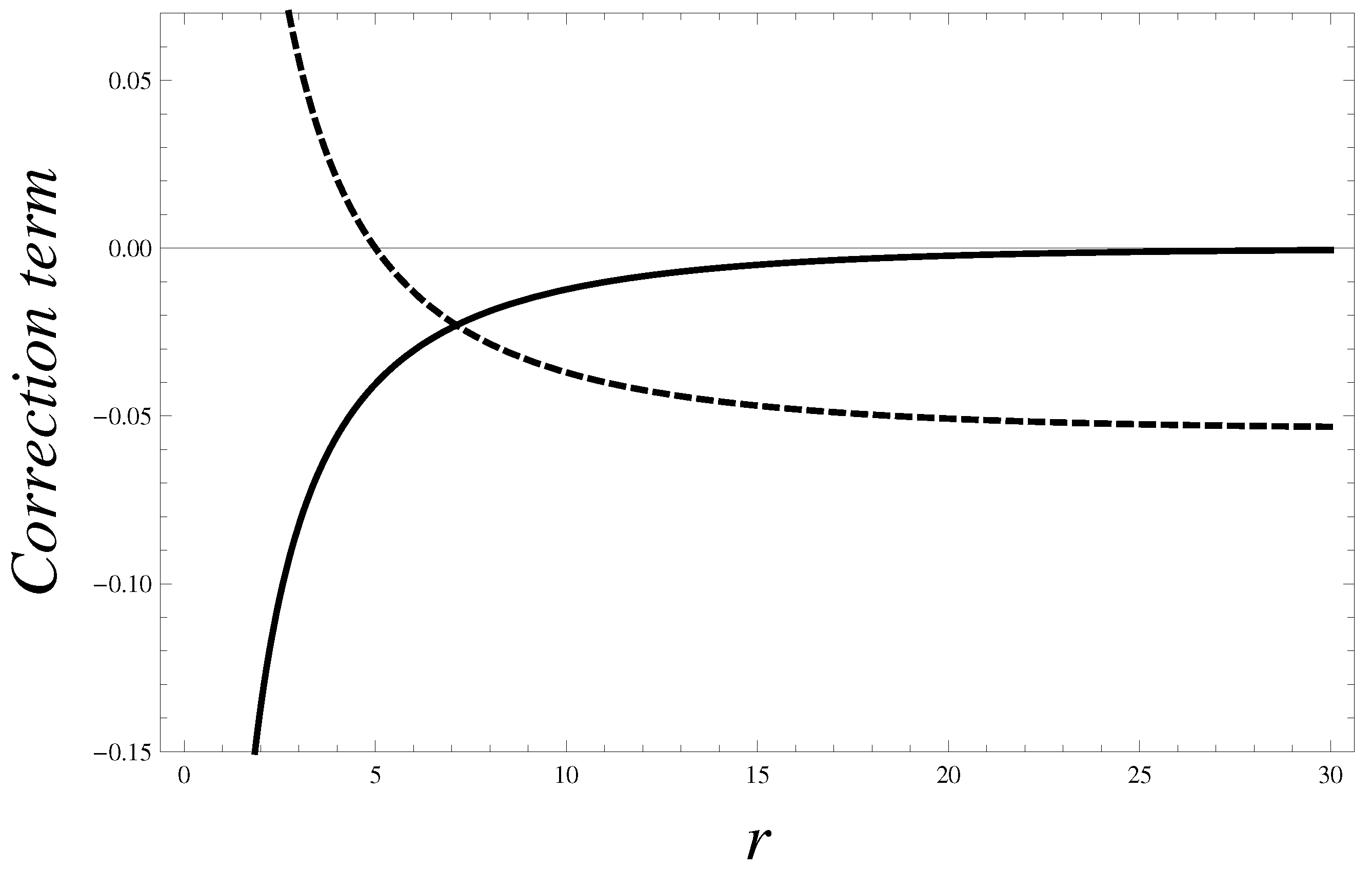
We comment about the physical behavior of potential Equation (92) and we want to add some reflections considering the result of the rotation curve shown above. Before to analyze the mathematical properties of metric linked to potential Equation (92), we want to show the different values of correction to the Newtonian potential. In 
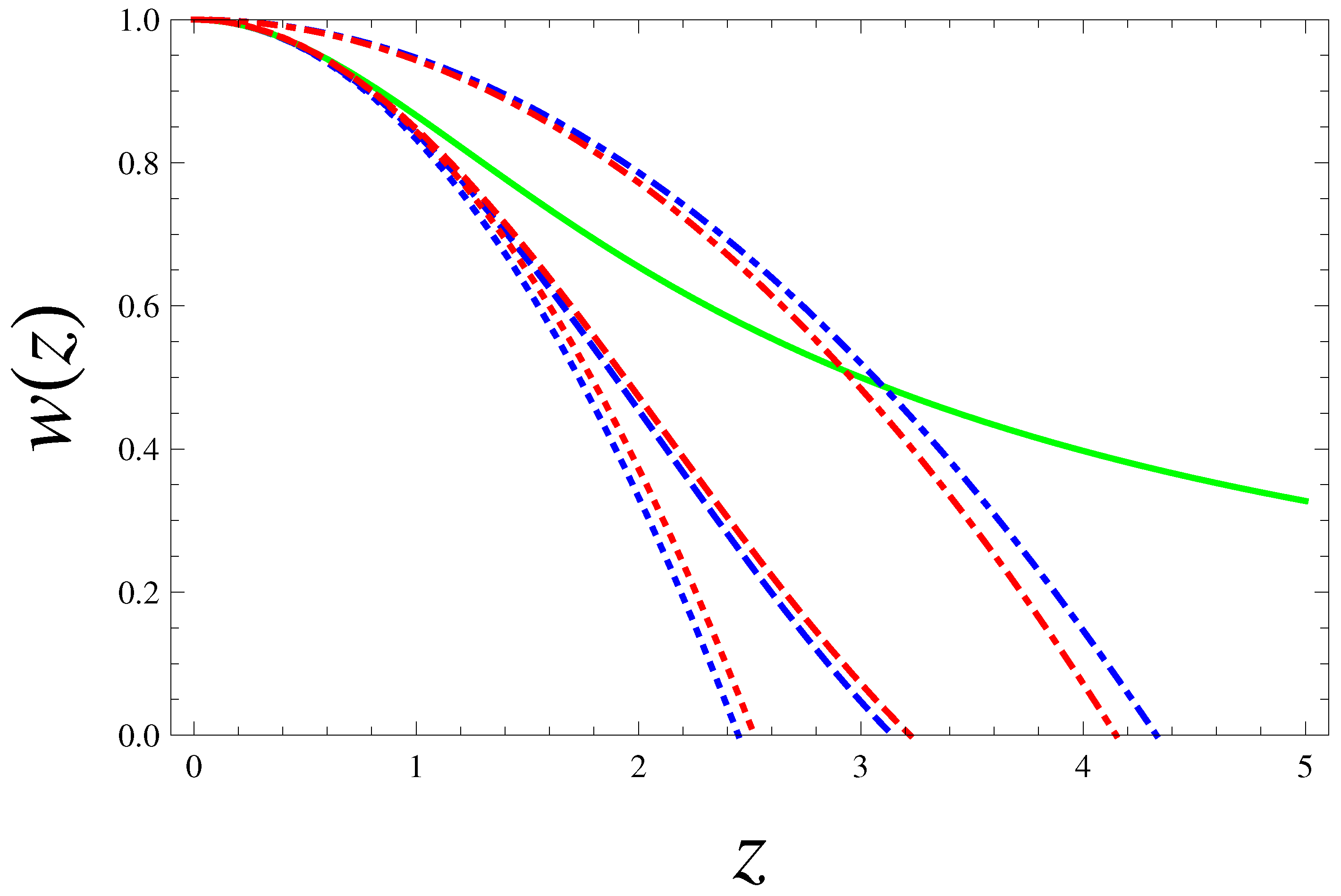
Figure 10 we report the radial behavior of the corrections to 1 / r for the potentials Equation (38) and Equation (92) (to minimize the difference we considered only f ( R ) -gravity). From the plot we note a discrepancy between the two corrections. The correction by R R 2 6 μ 1 2 -gravity acts over distances much smaller, while the correction induced by R n -gravity provides a potential nearly constant over large intervals and slowly goes to zero ( r β 1 ). For this aspect the potential Equation (92) does not need the DM component. Then with a procedure of fine tuning of r c and β it was possible to justify the experimental rotation curve for a wide class of galaxies [62] when n = 3 . 5 . This choice was possible because there must be a relationship β = β ( n ) so that the potential Equation (92) was compatible with respect to the field equations. These are the positive aspects of the potential Equation (92) used in [59,62].
Figure 10. Comparison between the corrective terms induced by f ( R ) -gravity ( e μ 1 r 3 r , solid line) and R n -gravity ( 1 ( r / r c ) β 2 r , dashed line). μ 1 = 0 . 1 , β = 0 . 8 and r c = 5 . The unities for r c and μ 1 are arbitrary. The dashed curve shows a very slow ascent.
Galaxies 02 00520 g010
We conclude this section by reviewing the fundamental weaknesses of R n -gravity.
  • The potential Equation (92) presents an analogous behavior of potential Equation (38). In fact for r < r c one has 1 ( r / r c ) β 2 r > 0 then the correction is “repulsive” like one induced by Ricci tensor square, while for r > r c one has an attractive correction. Now by remembering the reason of extension of GR, now we have unlike a repulsive contribution for r < r c . If in f ( X , Y , Z ) -gravity we can delete the Ricci tensor square contribution and we have only the f ( R ) -gravity, in R n -gravity we must collapse only in GR.
  • The potential Equation (92) belongs to general class of solutions for R n -gravity classified by a perturbative method [58], but the solutions are n-independent. Obviously the general solutions (it would be hard challenge to find them) are n-dependent, but at first order with respect to the perturbative parameter and in the vacuum (This parameter is generally c 2 , but the analysis is the same if we consider the dimensionless ratio r g / r ) the field equations are identically vanishing. So we say that the presence of matter has been not considered and the choice of arbitrary constant has been evaluated only by matching R n -gravity with GR in the limit β 0 . In fact by solving the field equations correctly in presence of matter (also with the point-like source) we would obtain solutions depending on the perturbative parameter and the technique is misplaced.
For these two aspects, but especially for the second point, R n -gravity does not admit the Newtonian limit if n 1 . The potential Equation (92) does not follow a correct framework when extending the GR to the new theories we want to generalize the Newtonian potential. Generally all theories without Ricci scalar in the Lagrangian suffer from the same problem. For example also R 2 -gravity is in the same situation: is not possible to extend the solution in the matter [58]. Although we have solutions as 1 / r with additional asymptotically flat terms, it is not automatic the assertion that these solutions are the Newtonian limit of theory.
Let us analyze now the mathematical properties of the metric trying to justify the difference of spatial behaviors in Figure 10. To simplify the calculation we choose the set of the standard coordinates. The metric Equation (21), from the expressions Equation (38), becomes (The set of standard coordinates is defined by the condition to obtain the standard definition of the circumference with radius r. From the metric tensor Equation (21) we must impose the condition 1 2 Ψ ( r ) r 2 = r ˜ 2 for the new radial coordinate)
d s 2 = 1 r g r 1 + 1 3 e μ 1 r 4 3 e μ 2 r d t 2 + 1 + r g r 1 μ 1 r + 1 3 e μ 1 r 2 ( μ 2 r + 1 ) 3 e μ 2 r d r 2 r 2 d Ω
where d Ω = d θ 2 + sin 2 θ d ϕ 2 is the solid angle, while the element of distance linked to potential Equation (92) can be written as follows
d s 2 = 1 + 2 Φ R n S C ( r ) d t 2 1 2 Ψ R n S C ( r ) d r 2 r 2 d Ω
where Φ R n S C ( r ) is the the potential Equation (92) and Ψ R n S C ( r ) is the other potential missing in the paper [62]. The metrics Equation (93) and Equation (38) represent the same space-time at first order of r g / r . However, in their analysis the knowledge of last potential is useless because its contribution in the geodesic motion is at fourth order. By following the paradigm of weak field limit at small velocity [55,56,57] for the R n -gravity we find
Ψ R n S C ( r ) = G M + K ( β ) + K X r + β 1 4 G M r r r c β + 1 4 r d r r 2 R ( r )
where K ( β ) and K X are constants depending, respectively, on the value of β and on the integral operation, while the Ricci scalar R could be an arbitrary function. In fact it needs some comment about the index n in the Ricci scalar. If n is a integer number, then the Ricci scalar can assume any value and can be also a generic space depending function. More attention is needed if n is a rational number. The field Equation (56) take into account up to third derivatives with respect to the Ricci scalar, then we must ensure that the function f ( R ) and its derivatives are always well defined [58]. In this case for n < 3 the solution Ricci flat ( R = 0 ) or space depending and asymptotically vanishing are excluded. Only solutions with constant values are allowed, but the algebraic sign is crucial. A such behavior is expected any time we have the condition lim R 0 f ( R ) = constant [58]. Now in all these considerations we do not recover the condition lim r Ψ R n S C ( r ) = 0 : then we have a theory which does not provide the Minkowskian limit. It is using the first perturbative contribution of a metric component (providing the flatness at infinity), while other contributions in the remaining metric components (negligible in the Newtonian limit) do not cover the same asymptotic limit. Then only for n > 3 we can have the flatness at infinity.
Then we could say that for n > 3 the Minkowskian limit is recovered but a such perturbative approach can be performed only in the vacuum. The objection previously shown comes back. Up to third order ( c 6 or r g 3 ) the geometrical side of field equation is identically null, but the matter side could not be null at first order ( c 2 or r g ).
The class of R n -gravity are examples of theories where the weak field limit procedure does not generate automatically the Minkowskian limit. In fact only if we consider theories satisfying the condition lim X 0 f ( R ) = 0 [58], their weak field limit is compatible with the request of asymptotically flatness. Moreover f ( R ) -gravity mimicking an additional source due to its scalar curvature [55,56,60] we would have a constant matter that pervades all space giving us a justification of more intense gravitational potential. In addition if lim R 0 f ( R ) = costant we do not have the Minkowskian limit, but we can interpret the apparent mass, only from the experimental point of view, as DM. These aspects, then, can be a mathematical motivation for different shape of point-like gravitational potential, but also source of further attention.

6. The Gravitational Lensing in f ( X , Y , Z ) -Gravity

Gravitational lensing can be considered as one of the main probes for DM at galactic and extragalactic level. However, modified gravity could affect the lensing quantities vs. DM. Let us develop this issue in the framework of Fourth Order Gravity.

6.1. The Point-Like Source

Let us start by defining the Lagrangian of a photon moving in the gravitational field with metric Equation (93). It is
L = 1 2 1 r g r Ξ ( r ) t ˙ 2 1 + r g r Λ ( r ) r ˙ 2 r 2 θ ˙ 2 r 2 sin 2 θ ϕ ˙ 2
where Ξ ( r ) 1 + Ξ ^ ( r ) 1 + 1 3 e μ 1 r 4 3 e μ 2 r , Λ ( r ) 1 + Λ ^ ( r ) 1 μ 1 r + 1 3 e μ 1 r 2 ( μ 2 r + 1 ) 3 e μ 2 r and the dot represents the derivatives with respect to the affine parameter λ. Since the variable θ does not have dynamics ( θ ¨ = 0 ) we can choose for simplicity θ = π / 2 . By applying the Euler-Lagrangian equation to Lagrangian Equation (96) for the cyclic variables t, ϕ we find two motion constants
L t ˙ = 1 r g r Ξ ( r ) t ˙ T L ϕ ˙ = r 2 ϕ ˙ J
and respect to λ we find the “energy” of Lagrangian (The Equation (96) is a quadratic form, so it corresponds to its Hamiltonian)
L = 0
By inserting the Equation (97) into Equation (98) we find a differential equation for r ˙
r ˙ ± = ± T 1 1 + r g r Λ ( r ) 1 1 r g r Ξ ( r ) J 2 r 2
r ˙ + is the solution for leaving photon, while r ˙ is one for incoming photon. Let r 0 be a minimal distance from the lens center (Figure 11). We must impose the condition r ˙ ± ( r 0 ) = 0 from the which we find
J 2 = r 0 2 T 2 1 r g r 0 Ξ ( r 0 )
Figure 11. The gravitational lensing geometric for a point-like source lens L at distance D O L from observer O. A source S at distance D O S from O has angular position β from the lens. A light ray (dashed line) from S which passes the lens at minimal distance r 0 is deflected by α; the observer sees an image of the source at angular position θ = b / D O L where b is the impact factor. D L S is the distance lens—source.
Galaxies 02 00520 g011
Now the deflection angle α (Figure 11) is defined by following relation
α = π + ϕ f i n = π + 0 ϕ f i n d ϕ = π + λ i n λ f i n ϕ ˙ d λ = π + λ i n λ 0 ϕ ˙ d λ + λ 0 λ f i n ϕ ˙ d λ = π + r 0 ϕ ˙ r ˙ d r + r 0 ϕ ˙ r ˙ + d r = π + 2 r 0 ϕ ˙ r ˙ + d r
where λ 0 is the value of λ corresponding to the minimal value ( r 0 ) of radial coordinate r. By putting the expressions of J, ϕ ˙ and r ˙ + into Equation (101) we get the deflection angle
α = π + 2 r 0 d r r 1 1 + r g r Λ ( r ) 1 r g r Ξ ( r 0 ) 1 r g r Ξ ( r ) r 2 r 0 2 1
which in the case r g / r 1 (We do not consider the GL generated by a black hole) becomes
α = 2 r g 1 r 0 + F μ 1 , μ 2 ( r 0 )
where
F μ 1 , μ 2 ( r 0 ) 1 2 r 0 r 0 r 2 [ Λ ^ ( r ) Ξ ^ ( r ) ] + r 3 Ξ ^ ( r 0 ) r 0 3 Λ ^ ( r ) r 3 ( r 2 r 0 2 ) 1 r 0 2 r 2 d r
From the definition of Ξ ^ and Λ ^ we note that in the case f ( X , Y , Z ) R we obtain F μ 1 , μ 2 ( r 0 ) 0 . In a such way we extended and contemporarily recovered the outcome of GR.
The analytical dependence of function F μ 1 , μ 2 ( r 0 ) from the parameters μ 1 and μ 2 is given by evaluating the integral Equation (104). A such as integral is not easily evaluable from the analytical point of view. However, this aspect is not fundamental, since we can numerically appreciate the deviation from the outcome of GR. In fact in Figure 12 we show the plot of deflection angle Equation (103) by f ( X , Y , Z ) -gravity for a given set of values for μ 1 and μ 2 . The spatial behavior of α is ever the same if we do not modify μ 2 . This outcome is really a surprise: by the numerical evaluation of the function F μ 1 , μ 2 ( r 0 ) one notes that the dependence of μ 1 is only formal. If we solve analytically the integral we must find a μ 1 independent function. However, this statement should not be justified only by numerical evaluation but it needs an analytical proof. For these reasons in the next section we reformulate the theory of Gravitational Lensing (GL) generated by a generic matter distribution and demonstrate that for f ( R ) -gravity one has the same outcome of GR.
Figure 12. Comparison between the deflection angle of GR (solid line) and one of f ( X , Y , Z ) -gravity (dashed line) Equation (103) for a fixed value μ 2 = 2 and any μ 1 .
Galaxies 02 00520 g012

6.2. Extended Sources

In this section we want to recast the framework of GL for a generic matter source distribution ρ ( x ) so the photon can undergo many deviations. In this case we leave the hypothesis that the flight of photon belongs always to the same plane, but we consider only the deflection angle as the angle between the directions of incoming and leaving photon. Finally we find the generalization of GL in f ( X , Y , Z ) -gravity including the previous outcome of deflecting point-like source (and resolving the integral Equation (104)).
The starting point is the relativistic distance Equation (39) where Φ is given by the superposition principle Equation (41) and an analogous relation is valid also for Ψ. By introducing the four velocity u μ = x ˙ μ = ( u 0 , u ) the flight of photon is regulated by the condition
d s 2 = g α β u α u β = ( 1 + 2 Φ ) u 0 2 ( 1 2 Ψ ) | u | 2 = 0
then u μ is given by
u μ = 1 2 Ψ 1 + 2 Φ | u | , u
In the Newtonian limit we find that the geodesic motion equation becomes
u ˙ μ + Γ α β μ u α u β = 0 u ˙ + | u | 2 ( Φ + Ψ ) 2 u Ψ · u = 0
and by supposing | u | 2 = 1 we can recast the equation in a more known aspect
u ˙ = 2 Ψ + 1 2 ( Φ Ψ )
where = u | u | · u | u | is the two dimensions nabla operator orthogonal to direction of vector u . In GR we would had only u ˙ = 2 Φ since we have Ψ = Φ . In fact the field Equation (28) admit the pointlike solutions Equation (38) and the condition Equation (34) is satisfied [57]. We can affirm, then, that only in GR the metric potentials are equals (or more generally their difference must be proportional to function | x | 1 ). The constraint Equation (34) has been found also many times in the context of cosmological perturbation theory [100,101,102,103,104].
The deflection angle Equation (101) is now defined by equation
α = λ i λ f d u d λ d λ
where λ i and λ f are the initial and final value of affine parameter [105]. For a generic matter distribution we can not a priori claim that the deflection angle belongs to lens plane (as pointlike source), but we can only link the deflection angle to the difference between the initial and final velocity u . So we only analyze the directions of photon before and after the interaction with the gravitational mass. Then the Equation (109) is placed by assuming α = Δ u = u i u f . From the geodesic Equation (108) the deflection angle becomes
α = 2 λ i λ f Ψ + 1 2 ( Φ Ψ ) d λ
The Formula Equation (110) represents the generalization of deflection angle in the framework of GR. By considering the photon incoming along the z-axes we can set u i = ( 0 , 0 , 1 ) . Moreover we decompose the general vector x ϵ R 3 in two components: ξ ϵ R 2 and z ϵ R . The differential operator now can be decomposed as follows = + z ^ z = ξ + z ^ z , while the modulus of distance is | x x | = | ξ ξ | 2 + ( z z ) 2 Δ ( ξ , ξ , z , z ) . Since the potentials Φ , Ψ 1 , around the lens, the solution of Equation (108) with the initial condition u i = ( 0 , 0 , 1 ) can be expressed as follows
u = ( O ( Φ , Ψ ) , O ( Φ , Ψ ) , 1 + O ( Φ , Ψ ) )
and we can substitute the integration with respect to the affine parameter λ with z. In fact we note
d λ = d z d z / d λ = d z 1 + O ( Φ , Ψ ) d z
and the deflection angle Equation (110) becomes
α = z i z f ξ ( Φ + Ψ ) + z ^ z ( Φ Ψ ) d z
From the expression of potentials for a generic matter distribution (see potential Equation (41) where f X ( 0 ) = 1 for example) we find the relations
Φ + Ψ = 2 G d 2 ξ d z ρ ( ξ , z ) Δ ( ξ , ξ , z , z ) + 2 G d 2 ξ d z ρ ( ξ , z ) Δ ( ξ , ξ , z , z ) e μ 2 Δ ( ξ , ξ , z , z ) Φ Ψ = 2 G 3 d 2 ξ d z ρ ( ξ , z ) Δ ( ξ , ξ , z , z ) e μ 1 Δ ( ξ , ξ , z , z ) e μ 2 Δ ( ξ , ξ , z , z )
and the deflection angle Equation (110) becomes
α = 2 G z i z f d 2 ξ d z d z ρ ( ξ , z ) ( ξ ξ ) Δ ( ξ , ξ , z , z ) 3 + 2 G z i z f d 2 ξ d z d z ρ ( ξ , z ) [ 1 + μ 2 Δ ( ξ , ξ , z , z ) ] Δ ( ξ , ξ , z , z ) 3 e μ 2 Δ ( ξ , ξ , z , z ) ( ξ ξ ) + + 2 G 3 z ^ z i z f d 2 ξ d z d z ρ ( ξ , z ) ( z z ) Δ ( ξ , ξ , z , z ) 3 [ 1 + μ 1 Δ ( ξ , ξ , z , z ) e μ 1 Δ ( ξ , ξ , z , z ) + 1 + μ 2 Δ ( ξ , ξ , z , z ) e μ 2 Δ ( ξ , ξ , z , z ) ]
In the case of hypothesis of thin lens belonging to plane ( x , y ) we can consider a weak dependence of modulus Δ ( ξ , ξ , z , z ) into variable z so there is only a trivial error if we set z = 0 . With this hypothesis the integral into z is incorporated by definition of two dimensional mass density Σ ( ξ ) = d z ρ ( ξ , z ) . Since we are interested only to the GL performed by one lens we can extend the integration range of z between ( , ) . Now the deflection angle is the following
α = 4 G d 2 ξ Σ ( ξ ) 1 | ξ ξ | | ξ ξ | F μ 2 ( ξ , ξ ) ξ ξ | ξ ξ |
where
F μ 2 ( ξ , ξ ) = 0 d z ( 1 + μ 2 Δ ( ξ , ξ , z , 0 ) ) Δ ( ξ , ξ , z , 0 ) 3 e μ 2 Δ ( ξ , ξ , z , 0 )
The last integral in Equation (115) is vanishing because the integrating function is odd with respect to variable z. The expression Equation (116) is the generalization of outcome Equation (103) and mainly we found a correction term depending only on the μ 2 parameter.
In the case of point-like source Σ ( ξ ) = M δ ( 2 ) ( ξ ) we find
α = 2 r g 1 | ξ | | ξ | F μ 2 ( ξ , 0 ) ξ | ξ |
and in the case of f ( X , Y , Z ) f ( R ) (i.e., μ 2 and F μ 2 ( ξ , ξ ) 0 ) we recover the outcome of GR α = 2 r g ξ / | ξ | 2 . From the theory of GL in GR we know that the deflection angle 2 r g / r 0 is formally equal to 2 r g / | ξ | if we suppose r 0 = | ξ | . Besides both r 0 , | ξ | are not practically measurable, while it is possible to measure the so-called impact parameter b (see Figure 11). But only in the first approximation these three quantities are equal.
In fact when the photon is far from the gravitational source we can parameterize the trajectory as follows
t = λ x = t y = b r = t 2 + b 2 ϕ = arctan b t
and from the definition of angular momentum Equation (97) in the case of t b we have
J = ϕ ˙ r 2 = b / t 2 1 + b 2 / t 2 ( t 2 + b 2 ) b
By using the condition Equation (100) r ˙ ± ( r 0 ) = 0 we find the relation among b and r 0 (The constant T is dimensionless if we consider that λ is the length of trajectory of photon. In this case without losing the generality we can choose T = 1 )
b = r 0 T 1 r g r 0 Ξ ( r 0 ) r 0
justifying then the position r 0 = | ξ | in the limit r g / r 1 (but also r g / r 0 1 ).
In Figure 13 we report the plot of deflection angle Equation (118). The behaviors shown in figure are parameterized only by μ 2 and we note an equal behavior shown in Figure 12.
With the expression Equation (118) we have the analytical proof of statement at the end of previous section. In fact in the Equation (118) we have not any information about the correction induced in the action Equation (18) by a generic function of Ricci scalar ( f X X 0 ). This result is very important if we consider only the class of theories f ( R ) -gravity. In this case, since μ 2 , we found the same outcome of GR. From the behavior in Figure 13 we note that the correction to outcome of GR is deeply different for r 0 0 , while for r 0 the behavior Equation (118) approaches the outcome of GR, but the deviations are smaller. This difference is given by the repulsive correction to the gravitational potential (see metric Equation (39)) induced by f ( Y , Z ) . Only by leaving the thin lens hypothesis (the lens does not belong to plane z = 0 ) we can have the deflection angle depending by μ 1 Equation (115). In fact in this case the third integral in Equation (115) is not zero. Then in the case of thin lens we have a complete degeneracy of results: f ( R ) -gravity equivalent to the GR in the thin lens case (see also [68]). In order to find some differences, we must include the contributions generated by the squared Ricci tensor. However, also in this case we do not get the right behavior: the deflection angle is smaller than the one in GR. Furthermore f ( X , Y , Z ) -gravity does not mimic the DM component by assuming the thin lens hypothesis.
A final remark is order at this point. The fact that f ( R ) gravity and GR give the same lensing effects is due to the fact that the corrections induced by f ( R ) on the g t t and g i j components of the metric (that is the potentials Φ and Ψ) are opposite and cancel out as demonstrated in details in [67,68]. This means that the only GR contribution remains in the deflection angle.
Figure 13. Comparison between the deflection angle of GR (solid line) and of f ( X , Y , Z ) -gravity (dashed line) Equation (118) for 0 . 2 < μ 2 < 2 .
Galaxies 02 00520 g013

6.3. The Lens Equation

In order to demonstrate the effect of a deflecting mass, let us show the simplest GL configuration in Figure 11. A point-like mass is located at a distance D O L from the observer O. The source is at distance D O S from the observer, and its true angular separation from the lens L is β, the separation which would be observed in the absence of lensing ( r g = 0 ). The photon which passes the lens at distance r 0 b is deflected with an angle α.
Since the deflection angle Equation (103) is equal to Equation (118), for sake of simplicity we will use the “vectorial” expression. Then the expression Equation (118), by considering the relation Equation (121), becomes
α = 2 r g 1 b b F μ 2 ( b , 0 )
The condition that this photon reach the observer is obtained from the geometry of Figure 11. In fact we find
β = θ D L S D O S α
Here D L S is the distance of the source from the lens. In the simple case with a Euclidean background metric here, D L S = D O S D O L ; however, since the GL occurs in the Universe on large scale, one must use a cosmological model [105]. Denoting the angular separation between the deflecting mass and the deflected photon as θ = b / D O L the lens equation for f ( X , Y , Z , ) -gravity is the following
[ 1 + θ E 2 F ( θ ) ] θ 2 β θ θ E 2 = 0
where θ E = 2 r g D L S D O L D O S is the Einstein angle and
F ( θ ) = 0 d z ( 1 + μ 2 D O L θ 2 + z 2 ) ( θ 2 + z 2 ) 3 e μ 2 D O L θ 2 + z 2 )
Since we have 0 < θ 2 F ( θ ) < 1 (Figure 14) we can find a perturbative solution of Equation (124) by starting from one in GR, θ ± G R = β ± β 2 + 4 θ E 2 2 . In fact by assuming θ = θ ± G R + θ * and neglecting θ * 2 F ( θ * ) in Equation (124) we find
θ = θ ± G R θ E 2 β 2 + 4 θ E 2 F ( θ ± G R ) θ ± G R 2
and in the case of β = 0 we find the modification to the Einstein ring
θ = ± θ E 1 θ E 2 2 F ( θ E )
In Figure 15 we show the angular position of images with respect to the Einstein ring. Both the deflection angle and the position of images assume a smaller value than ones of GR. Then the corrections to the GR quantities are found only for the introduction in the action Equation (18) of curvature invariants Y (or Z), while there are no modifications induced by adding a generic function of Ricci scalar X. The algebraic signs of terms concerning the parameter μ 2 are ever different with respect to the terms of GR in Equation (38) and they can be interpreted as a “repulsive force” giving us a minor curvature of photon. The correction terms concerning the parameter μ 1 have opposite algebraic sign in the metric component g t t and g i j Equation (38) and we lose their information in the deflection angle Equation (113).
In both approaches we find the same outcomes μ 1 -independent because the matter source (in our case it is a point-like mass) is symmetric with respect to z-axes and we neglect the second integral in Equation (115). Obviously for a generic matter distribution the deflection angle is defined by Equation (115) and the choice of second derivative of function of Ricci scalar is not arbitrary anymore.
Figure 14. Plot of function θ 2 F ( θ ) Equation (125) for 1 < μ 2 D O L < 10 .
Galaxies 02 00520 g014
Figure 15. Plot of the Einstein ring (solid line) and its modification Equation (127) in the f ( X , Y , Z ) -gravity for 1 < μ 2 D O L < 10 (dashed line).
Galaxies 02 00520 g015

7. Conformal Transformations in the Weak Field Limit

As a final issue, let us discuss the conformal transformations in the weak field limit approximation. It is important to stress that we developed all the above considerations in the Jordan frame in order to control the behavior of the standard matter that, in this frame, remains minimally coupled. In the Einstein frame, the matter is non-minimally coupled and this fact could give rise to some difficulties in order to control the dynamics. Clearly, this means that all the considered modifications insist on the geometric part. Controlling the relation between physical quantities passing from a frame to another could give hints to understand if conformal transformations are only a mathematical tool or have some physical meaning (see [21] for a detailed discussion).

7.1. Scalar Tensor Gravity in the Jordan Frame

Let us start by considering the action of the scalar-tensor gravity in 4 dimensions. It is
A J F = d 4 x g ϕ R + V ( ϕ ) + ω ( ϕ ) ϕ ; α ϕ ; α + X L m
Let us note that the action
A J F = d 4 x g F ( ϕ ) R + V ( ϕ ) + ω ( ϕ ) ϕ ; α ϕ ; α + X L m
is apparently more general than Equation (128). In fact by substituiting F ( ϕ ) ϕ , we obtain only a new definition of functions ω ( ϕ ) and V ( ϕ ) so the two formulations are essentially equivalent.
The term L m is the minimally coupled ordinary matter contribution considered as a perfect fluid; ω ( ϕ ) is a function of the scalar field and V ( ϕ ) is its potential which specifies the dynamics. Actually if ω ( ϕ ) = ± 1 , 0 the nature and the dynamics of the scalar field is fixed. It can be a canonical scalar field, a phantom field or a field without dynamics (see e.g., [106,107] for details). In the metric approach, the field equations are obtained by varying the action Equation (128) with respect to g μ ν and ϕ. The field equations are
ϕ R μ ν ϕ R + V ( ϕ ) + ω ( ϕ ) ϕ ; α ϕ ; α 2 g μ ν + ω ( ϕ ) ϕ ; μ ϕ ; ν ϕ ; μ ν + g μ ν ϕ = X T μ ν 2 ω ( ϕ ) ϕ + ω ϕ ( ϕ ) ϕ ; α ϕ ; α R V ϕ ( ϕ ) = 0
and the trace equation is
ϕ R + 2 V ( ϕ ) + ω ( ϕ ) ϕ ; α ϕ ; α 3 ϕ = X T
Here we introduced V ϕ = d V d ϕ and ω ϕ ( ϕ ) = d ω ( ϕ ) d ϕ . If we assume that the Lagrangian density L m of matter depends only on the metric components g μ ν and not on its derivatives, we obtain T μ ν = 1 / 2 L m g μ ν δ L m / δ g μ ν . Let us consider a source with mass M. The energy-momentum tensor is the same of Equation (35) and Equation (36). It is useful to get the expression of L m . In fact from the definition of energy momentum tensor we have
δ d 4 x g L m = d 4 x g T μ ν δ g μ ν = d 4 x g ρ u μ u ν δ g μ ν
and further from the mathematical properties of metric tensor we have
δ ( g ρ ) = 1 / 2 g ρ u μ u ν δ g μ ν = 1 / 2 g ρ u μ u ν δ g μ ν
then we find
L m = 2 ρ
The variation of density is given by
δ ρ = ρ 2 ( g μ ν u μ u ν ) δ g μ ν
order to deal with standard self-gravitating systems, any theory of gravity has to be developed in its Newtonian or post-Newtonian limit depending on the order of approximation in terms of squared velocity v 2 [58].
In this context, also the scalar field ϕ is approximated as the Ricci scalar. In particular we get ϕ = ϕ ( 0 ) + ϕ ( 2 ) + while the functions V ( ϕ ) and ω ( ϕ ) can be substituted by their corresponding Taylor series.
From the lowest order of field Equation (130) we have
V ( ϕ ( 0 ) ) = 0 , V ϕ ( ϕ ( 0 ) ) = 0
and also in the scalar tensor gravity a missing cosmological component in the action Equation (128) implies that the space-time is asymptotically Minkowskian; moreover the ground value of scalar field ϕ must be a stationary point of potential. In the Newtonian limit, we have
Φ ϕ ( 2 ) ϕ ( 0 ) R ( 2 ) 2 = X ρ ϕ ( 0 ) Ψ + ϕ ( 2 ) ϕ ( 0 ) + R ( 2 ) 2 δ i j + { Ψ Φ ϕ ( 2 ) ϕ ( 0 ) } , i j = 0 ϕ ( 2 ) + V ϕ ϕ ( ϕ ( 0 ) ) 2 ω ( ϕ ( 0 ) ) ϕ ( 2 ) + R ( 2 ) 2 ω ( ϕ ( 0 ) ) = 0 R ( 2 ) + 3 ϕ ( 2 ) ϕ ( 0 ) = X ρ ϕ ( 0 )
These equations are not simply the merging of field equations of GR and a further massive scalar field, but come out to the fact that the scalar tensor gravity generates a coupled system of equations with respect to Ricci scalar R and scalar field ϕ. The gravitational potentials Φ, Ψ and the Ricci scalar R ( 2 ) are given by
Φ ( x ) = X 4 π ϕ ( 0 ) d 3 x ρ ( x ) | x x | 1 8 π d 3 x R ( 2 ) ( x ) | x x | + ϕ ( 2 ) ( x ) ϕ ( 0 ) Ψ ( x ) = Φ ( x ) + ϕ ( 2 ) ( x ) ϕ ( 0 ) R ( 2 ) ( x ) = X ρ ( x ) ϕ ( 0 ) 3 ϕ ( 2 ) ( x ) ϕ ( 0 )
and supposing that 2 ω ( ϕ ( 0 ) ) ϕ ( 0 ) 3 0 we find for the scalar field ϕ ( 2 ) the Yukawa-like field equation
m ϕ 2 ϕ ( 2 ) = X ρ 2 ω ( ϕ ( 0 ) ) ϕ ( 0 ) 3
where we introduced the mass definition
m ϕ 2 ϕ ( 0 ) V ϕ ϕ ( ϕ ( 0 ) ) 2 ω ( ϕ ( 0 ) ) ϕ ( 0 ) 3
It is important to stress that the potential Ψ can be found also as
Ψ ( x ) = 1 8 π d 3 x R ( 2 ) ( x ) | x x | ϕ ( 2 ) ( x ) ϕ ( 0 )
see for example [108]. By using the Fourier transformation, the solution of Equation (139) has the following form
ϕ ( 2 ) ( x ) = X 2 ω ( ϕ ( 0 ) ) ϕ ( 0 ) 3 d 3 k ( 2 π ) 3 / 2 ρ ˜ ( k ) e i k · x k 2 + m ϕ 2
The expressions Equation (138) and Equation (142) represent the most general solution of any scalar-tensor gravity in the Newtonian limit. Since the superposition principle is yet valid (as previously analyzed), it is sufficient to consider again the solutions generated by the pointlike source. Then the solutions are [57,58,108]
ϕ ( 2 ) ( x ) = 1 2 ω ( ϕ ( 0 ) ) ϕ ( 0 ) 3 r g | x | e m ϕ | x | R ( 2 ) ( x ) = 4 π r g ϕ ( 0 ) δ ( x ) + 3 m ϕ 2 [ 2 ω ( ϕ ( 0 ) ) ϕ ( 0 ) 3 ] ϕ ( 0 ) r g | x | e m ϕ | x | Φ ( x ) = G M ϕ ( 0 ) | x | 1 e m ϕ | x | 2 ω ( ϕ ( 0 ) ) ϕ ( 0 ) 3 Ψ ( x ) = G M ϕ ( 0 ) | x | 1 + e m ϕ | x | 2 ω ( ϕ ( 0 ) ) ϕ ( 0 ) 3
In the case V ( ϕ ) = 0 , the scalar field is massless and ω ( ϕ ) = ω 0 / ϕ , we obtain
Φ ( x ) = Φ B D ( x ) = G M ϕ ( 0 ) | x | 2 ( 2 + ω 0 ) 2 ω 0 + 3 = G * M | x | Ψ ( x ) = Ψ B D ( x ) = G * M | x | 1 + ω 0 2 + ω 0
the well-known Brans-Dicke solutions [41] with Eddington’s parameter γ = 1 + ω 0 2 + ω 0 [70] where the gravitational constat is defined as G G * = G ϕ ( 0 ) 2 ( 2 + ω 0 ) 2 ω 0 + 3 .

7.2. Scalar Tensor Gravity in the Einstein Frame

Let us now introduce the conformal transformation
g μ ν g ˜ μ ν = Ω 2 g μ ν
where Ω = Ω ( x ) is a nowhere vanishing, regular function, called a Weyl or conformal transformation. This transformation has been introduced to show that scalar-tensor theories are, in general, conformally equivalent to the Einstein theory plus minimally coupled scalar fields. However, if standard matter is present, the conformal transformation generates the non-minimal coupling between the matter component and the scalar field.
By applying the transformation Equation (145), the action in Equation (128) can be reformulated as follows
A E F = d 4 x g ˜ Ξ R ˜ + W ( ϕ ˜ ) + ω ˜ ( ϕ ˜ ) ϕ ˜ ; α ϕ ˜ ; α + X L ˜ m
in which R ˜ is the Ricci scalar relative to the metric g ˜ μ ν and Ξ is a generic constant. The two actions Equation (128) and Equation (146) are mathematically equivalent. In fact the conformal transformation is given by imposing the condition
g ϕ R + V ( ϕ ) + ω ( ϕ ) ϕ ; α ϕ ; α + X L m = g ˜ Ξ R ˜ + W ( ϕ ˜ ) + ω ˜ ( ϕ ˜ ) ϕ ˜ ; α ϕ ˜ ; α + X L ˜ m
The relations between the quantities in the two frames are
ω ˜ ( ϕ ˜ ) d ϕ ˜ 2 = Ξ 2 [ 2 ϕ ω ( ϕ ) 3 ] d ϕ ϕ 2 W ( ϕ ˜ ) = Ξ 2 ϕ ( ϕ ˜ ) 2 V ( ϕ ( ϕ ˜ ) ) L ˜ m = Ξ 2 ϕ ( ϕ ˜ ) 2 L m Ξ g ˜ ρ σ ϕ ( ϕ ˜ ) ϕ Ω 2 = Ξ
The field equations for the new fields g ˜ μ ν and ϕ ˜ are
Ξ R ˜ μ ν Ξ R ˜ + W ( ϕ ˜ ) + ω ˜ ( ϕ ˜ ) ϕ ˜ ; α ϕ ˜ ; α 2 g ˜ μ ν + ω ˜ ( ϕ ˜ ) ϕ ˜ ; μ ϕ ˜ ; ν = X T ˜ μ ν 2 ω ˜ ( ϕ ˜ ) ˜ ϕ ˜ + ω ˜ ϕ ˜ ( ϕ ˜ ) ϕ ˜ ; α ϕ ˜ ; α W ϕ ˜ ( ϕ ˜ ) X δ L ˜ m δ ϕ ˜ = 0 Ξ R ˜ + 2 W ( ϕ ˜ ) + ω ˜ ( ϕ ˜ ) ϕ ˜ ; α ϕ ˜ ; α = X T ˜
where T ˜ μ ν and ˜ are the re-definition of the quantities Equation (35) with respect to the metric g ˜ μ ν . The field Equation (149) can be obtained from Equation (130) by substituing all geometrical and physical quantities in terms of conformally transformed ones. In particular we have
R μ ν = R ˜ μ ν + 2 ln Ω ; μ ν ˜ + 2 ln Ω ; μ ln Ω ; ν + [ ˜ ln Ω 2 ln Ω ; σ ln Ω ; σ ˜ ] g ˜ μ ν R = Ω 2 R ˜ + 6 ˜ ln Ω 3 ln Ω ; σ ln Ω ; σ ˜ ϕ ; μ ν = ϕ ; μ ν ˜ + 2 ϕ ; μ ϕ ; ν ln Ω ; σ ϕ ; σ ˜ g ˜ μ ν ( · ) = Ω 2 ˜ ( · ) 2 ln Ω ; σ σ ˜ ( · )
The integration of field Equation (149) is only formal because we do not know the analytical expression of the coupling function between the matter and the scalar field ϕ ˜ (see the third line of Equation (148)). We can make some assumptions on the parameter Ξ and the function ω ˜ ( ϕ ˜ ) in the minimally coupled Lagrangian Equation (146) and on the function ω ( ϕ ) in the nonminimally coupled Lagrangian Equation (128). If we choose ω ˜ ( ϕ ˜ ) = 1 / 2 , Ξ = 1 and ω ( ϕ ) = ω 0 / ϕ , the transformation between the scalar fields ϕ and ϕ ˜ is given by the first line in Equation (148), that is
ϕ ˜ ( ϕ ) = ϕ ˜ 0 + 2 ω 0 + 3 ln ϕ ϕ ( ϕ ˜ ) = exp ϕ ˜ ϕ ˜ 0 2 ω 0 + 3
where obviously ω 0 > 3 / 2 and ϕ ˜ 0 is an integration constant (Without losing generality, we can set ϕ ˜ 0 = 0 ). The potential W and the matter Lagrangian L ˜ m are
W ( ϕ ˜ ) = exp 2 ϕ ˜ 2 ω 0 + 3 V e ϕ ˜ 2 ω 0 + 3 L ˜ m = 2 ρ exp 2 ϕ ˜ 2 ω 0 + 3
In both frames, the scalar fields are expressed as perturbative contributions on the cosmological background ( ϕ ( 0 ) , ϕ ˜ ( 0 ) ) with respect to the dimensionless quantity v 2 . Then also for the scalar field ϕ ˜ , we can consider the develop ϕ ˜ = ϕ ˜ ( 0 ) + ϕ ˜ ( 2 ) + . Such a develop can be applied to the transformation rule Equation (151) and we obtain
ϕ ˜ ( ϕ ) = 2 ω 0 + 3 ln ϕ = 2 ω 0 + 3 ln ϕ ( 0 ) + 2 ω 0 + 3 ϕ ( 0 ) ϕ ( 2 ) + ϕ ˜ ( 0 ) + ϕ ˜ ( 2 ) + ϕ ( ϕ ˜ ) = e ϕ ˜ 2 ω 0 + 3 = e ϕ ˜ ( 0 ) 2 ω 0 + 3 + e ϕ ˜ ( 0 ) 2 ω 0 + 3 2 ω 0 + 3 ϕ ˜ ( 2 ) + ϕ ( 0 ) + ϕ ( 2 ) +
Since we are interested in the Newtonian limit of field Equation (149), we can assume, for the conformally transformed metric g ˜ μ ν , an expression as Equation (39) but with some differences. In fact from the conformal transformation Equation (145) and from the last line of Equation (148), we have
g ˜ μ ν = ϕ g μ ν = ϕ ( 0 ) η μ ν + [ ϕ ( 0 ) g μ ν ( 2 ) + ϕ ( 2 ) η μ ν ] + = η ˜ μ ν + g ˜ μ ν ( 2 ) +
then the conformally transformed metric becomes
d s 2 = ( ϕ ( 0 ) + 2 Φ ˜ ) d t 2 ( ϕ ( 0 ) 2 Ψ ˜ ) δ i j d x i d x j
and the relation between the gravitational potentials in the two frames is
Φ ˜ ϕ ( 0 ) Φ = ϕ ( 2 ) 2 , Ψ ˜ ϕ ( 0 ) Ψ = ϕ ( 2 ) 2
Then the field Equation (149) become (With the assumptions of the metric Equation (155) the Ricci tensor R ˜ μ ν in the Newtonian limit has the form Φ ˜ ϕ ( 0 ) (a similar behaviour for R ˜ i j ( 2 ) ), where the Ricci scalar is scaled by the factor ϕ ( 0 ) 2 . The same scaling occurs for the Laplacian: ϕ ( 0 ) )
Φ ˜ ϕ ( 0 ) R ˜ ( 2 ) 2 ϕ ( 0 ) = X T ˜ 00 ( 2 ) Ψ ˜ ϕ ( 0 ) + R ˜ ( 2 ) 2 ϕ ( 0 ) δ i j + ( Ψ ˜ Φ ˜ ) , i j ϕ ( 0 ) = 0 ϕ ˜ ( 2 ) ϕ ( 0 ) W ϕ ˜ ϕ ˜ ( ϕ ˜ ( 0 ) ) ϕ ˜ ( 2 ) X δ L ˜ m δ ϕ ˜ ( 2 ) = 0 R ˜ ( 2 ) = X T ˜ ( 2 )
where also in this case we have W ( ϕ ˜ ( 0 ) ) = 0 and W ϕ ˜ ( ϕ ˜ ( 0 ) ) = 0 . However, these conditions are an obvious consequence of the conformal transformation of conditions V ( ϕ ( 0 ) ) = 0 and V ϕ ( ϕ ( 0 ) ) = 0 . In fact we can figure out that V ( ϕ ) ( ϕ ϕ ( 0 ) ) 2 and then W ( ϕ ˜ ) e ϕ ˜ 2 ω 0 + 3 ϕ ( 0 ) 2 which, by using relations Equation (153), satisfies the above conditions. Finally, we note that W ϕ ˜ ϕ ˜ ( ϕ ˜ ( 0 ) ) = V ϕ ϕ e ϕ ˜ ( 0 ) 2 ω 0 + 3 2 ω 0 + 3 = V ϕ ϕ ( ϕ ( 0 ) ) 2 ω 0 + 3 and by the definition of mass m ϕ 2 , given in Equation (140), we obtain W ϕ ˜ ϕ ˜ ( ϕ ˜ ( 0 ) ) = m ϕ 2 / ϕ ( 0 ) . Finally, the energy-momentum tensor T ˜ μ ν is given by the following expression
T ˜ μ ν = ρ exp 2 ϕ ˜ 2 ω 0 + 3 u ˜ μ u ˜ ν
where g ˜ μ ν u ˜ μ u ˜ ν = 1 then u ˜ 0 = ϕ ( 0 ) + 2 Φ ˜ . In the Newtonian limit, we find T ˜ 00 ( 2 ) = ρ / ϕ ( 0 ) and T ˜ ( 2 ) = ρ / ϕ ( 0 ) 2 . It remains only to calculate the source term δ L ˜ m / δ ϕ ˜ of the scalar field ϕ ˜ ( 2 ) . From the third line of Equation (148) and, by using the transformation rules Equation (151), we find the coupling between the scalar field and the ordinary matter
δ L ˜ m δ ϕ ˜ = δ δ ϕ ˜ e 2 ϕ ˜ 2 ω 0 + 3 L m e ϕ ˜ 2 ω 0 + 3 g ˜ ρ σ = 2 e 2 ϕ ˜ 2 ω 0 + 3 2 ω 0 + 3 L m ( · ) + e 2 ϕ ˜ 2 ω 0 + 3 δ L m ( · ) δ g μ ν δ g μ ν δ ϕ ˜ = 2 e 2 ϕ ˜ 2 ω 0 + 3 2 ω 0 + 3 L m ( · ) + e 2 ϕ ˜ 2 ω 0 + 3 L m ( · ) 2 ( g μ ν u μ u ν ) g ˜ μ ν δ ϕ ( ϕ ˜ ) δ ϕ ˜ = 2 e 2 ϕ ˜ 2 ω 0 + 3 2 ω 0 + 3 L m ( · ) + e 2 ϕ ˜ 2 ω 0 + 3 3 L m ( · ) 2 1 2 ω 0 + 3 = 1 2 e 2 ϕ ˜ 2 ω 0 + 3 2 ω 0 + 3 L m ( · ) = e 2 ϕ ˜ 2 ω 0 + 3 2 ω 0 + 3 ρ
Then the system of Equation (157) becomes
Φ ˜ = X ρ 2 Ψ ˜ = Φ ˜ m ϕ 2 ϕ ˜ ( 2 ) = X ρ ϕ ( 0 ) 2 ω 0 + 3
and their solutions in the case of pointlike source are
Φ ˜ = G M | x | Ψ ˜ = Φ ˜ ϕ ˜ ( 2 ) = 1 ϕ ( 0 ) 2 ω 0 + 3 r g | x | e m ϕ | x |
The difference in Equation (156) between the gravitational potentials is satisfied by using the expression of scalar field in the Jordan frame (first line of Equation (143)) where, obviously, we set ω ( ϕ ) = ω 0 / ϕ . In fact we find
Φ ˜ ϕ ( 0 ) Φ = G M 2 ω 0 + 3 e m ϕ | x | | x | = ϕ ( 2 ) 2
and an analogous relations is found also for the couples Ψ , Ψ ˜ . Furthermore we can check also the transformation rules Equation (151) and Equation (153) for the solutions Equation (143) and Equation (161) of the scalar fields ϕ , ϕ ˜ .
The redefinition of the gravitational constant G (as performed in the Jordan frame G G * in the case of Brans-Dicke theory [41]) is not available when we are interested to compare the outcomes in both frame. In fact the couple of potentials Φ , Φ ˜ differs not only from the dynamical contribution of the scalar field ( ϕ ( 2 ) ) but also from the definition of the gravitational constant. Furthermore, in the Einstein frame, the scalar field ϕ ˜ does not contribute (the coupling constant between R and ϕ ˜ is vanishing), then we find the same outcomes of GR with ordinary matter. However, by supposing the Jordan frame as starting point and coming back via conformal transformation, we find that the gravitational constant is not invariant and depends on the background value of the scalar field in the Einstein frame, that is G G e f f e ϕ ˜ ( 0 ) G .

7.3. The Analogy between the Scalar Tensor Gravity and f ( R ) -Gravity

Recently, several authors claimed that higher-order theories of gravity and among them, f ( R ) gravity, are characterized by an ill defined behavior in the Newtonian regime. In particular, it is discussed that Newtonian corrections of the gravitational potential violate experimental constraints since these quantities can be recovered by a direct analogy with Brans-Dicke gravity simply supposing the Brans-Dicke characteristic parameter ω 0 vanishing (see [50,51,52] for a discussion). Actually, the calculations of the Newtonian limit of f ( R ) -gravity, directly performed in a rigorous manner, have showed that this is not the case [56,57,58,109] and it is possible to discuss also the analogy with Brans-Dicke gravity. The issue is easily overcome once the correct analogy between f ( R ) -gravity and the corresponding scalar-tensor framework is taken into account. It is important mentioning that several important results already achieved in the Newtonian regime, see e.g., [110,111], are confirmed by these rigorous approach and only the wrong analogies are ruled out.
In literature, it is shown that f ( R ) gravity models can be rewritten in term of a scalar-field Lagrangian non-minimally coupled with gravity but without kinetic term implying that the Brans-Dicke parameter is ω ( ϕ ) = 0 . This fact is considered the reason for the ill-definition of the weak field limit that should be ω inside the Solar System.
Let us deal with the f ( R ) gravity formalism in order to set correctly the problem. The field Equation (56) can be recast in the framework of scalar-tensor gravity as son as we select a particular expression for the free parameters of the theory. The result is the so-called O’Hanlon theory [112] which can be written as
A O H J F = d 4 x g ϕ R + V ( ϕ ) + X L m
The field equations are obtained by starting from ones of Equation (130)
ϕ R μ ν ϕ R + V ( ϕ ) 2 g μ ν ϕ ; μ ν + g μ ν ϕ = X T μ ν R + V ϕ ( ϕ ) = 0 ϕ R + 2 V ( ϕ ) 3 ϕ = X T
By supposing that the Jacobian of the transformation ϕ = f R is non-vanishing, the two representations can be mapped one into the other considering the following equivalence
ω ( ϕ ) = 0 V ( ϕ ) = f f R R ϕ V ϕ ( ϕ ) 2 V ( ϕ ) = f R R 2 f
From the definition of the mass Equation (140) we have ϕ V ϕ ( ϕ ) 2 V ( ϕ ) = 3 m ϕ 2 ϕ ( 2 ) , then we have also f R R 2 f = 3 m ϕ 2 ϕ ( 2 ) and by performing the Newtonian limit on the function f [58], we get f R ( 0 ) R ( 2 ) = 3 m ϕ 2 ϕ ( 2 ) . The spatial evolution of Ricci scalar is obtained by solving the field Equation (56)
R ( 2 ) = 3 m ϕ 2 ϕ ( 2 ) f R ( 0 ) = m ϕ 2 r g f R ( 0 ) e m ϕ | x | | x |
without using the conformal transformation [57,58]. The solution for the potentials Φ , Ψ are obtained simply by setting ω ( ϕ ) = 0 in Equation (143) and ϕ ( 0 ) = f R ( 0 ) . In the case f ( R ) R , from the second line of Equation (165), V ( ϕ ) = 0 m ϕ = 0 and the solutions Equation (143) become the standard Schwarzschild solution in the Newtonian limit.
Finally, we can consider a Taylor expansion (The terms resulting from R n with n 3 do not contribute to the Newtonian order.) of the form f = f R ( 0 ) R ( 2 ) + f R R ( 0 ) 2 R ( 2 ) 2 so that the associated scalar field reads ϕ = f R ( 0 ) + f R R ( 0 ) R ( 2 ) . The relation between ϕ and R ( 2 ) is R ( 2 ) = ϕ f R ( 0 ) f R R ( 0 ) while the self-interaction potential (second line of Equation (165)) turns out the be V ( ϕ ) = ( ϕ f R ( 0 ) ) 2 2 f R R ( 0 ) satisfying the conditions V ( f R ( 0 ) ) = 0 and V ϕ ( f R ( 0 ) ) = 0 . In relation to the definition of the scalar field, we can opportunely identify f R ( 0 ) with a constant value ϕ ( 0 ) = f R ( 0 ) which justifies the previous ansatz for matching solutions in the limit of GR. Furthermore, the mass of the scalar field can be expressed in term of the Lagrangian parameters as m ϕ 2 = 1 3 ϕ ( 0 ) V ϕ ϕ ( ϕ ( 0 ) ) = f R ( 0 ) 3 f R R ( 0 ) . Also in this case the value of mass is the same obtained by solving the problem without invoking the scalar tensor analogy [57,58]. However, with this remark, it is clear the analogy between f ( R ) -gravity and a particular class of scalar tensor theories [112].
Finally, the above results have to be interpreted also with respect to results reported in [50,51,52]. In those works, the relation between f ( R ) gravity and scalar-tensor theories was used to compute the weak-field limit. Though f ( R ) gravity, in metric formalism, is related to the Brans-Dicke theory with ω 0 = 0 , the equivalence is not complete because f ( R ) has a non-trivial potential, which is not present in the original Brans-Dicke theory. The role of the potential is to introduce a length scale (as we found here) and then the post-Newtonian parameter γ develops a spatial dependence. In Refs. [50,51,52] this spatial dependence is discussed despite the fact that ω 0 = 0 . Note that formulas presented in [50,51,52] for the weak-field limit are in complete agreement with those presented here also if achieved with a different approach.

8. Discussion and Conclusions

The weak field limit of Extended Theories of Gravity has been discussed in view of some relevant astrophysical issues. In particular, we have considered the hydrostatic equilibrium of stars, the galactic rotation curves and the gravitational lensing. Finally, we have analyzed the relations between the Jordan and Einstein frames in the same limit and focused our attention on the relations linking the gravitational potentials in both frames.
Specifically, we have considered theories containing generic functions of the Ricci scalar R, the squared Ricci tensor R α β R α β and the squared Riemann tensor R α β γ δ R α β γ δ . We obtain the analogy, in the Newtonian limit, with the so-called Quadratic Lagrangian containing the squared Ricci scalar and the squared Ricci tensor in addition to the linear term R. All contributions to the field equations related to the squared Riemann curvature invariant can be expressed by the other two curvature invariants (squared Ricci tensor and squared Ricci scalar) via the Gauss-Bonnet invariant. It is straightforward to show that the spherically symmetric solutions show a Yukawa-like dependence with two characteristic lengths. An important result is that, for generic Fourth Order Gravity models, two non-equivalent metric potentials come out. In the limit f R , only the Newtonian potential is present as it has to be in GR. The presence of two gravitational potentials, together with the non-validity of the Birkhoff and Gauss theorems, are the main differences between Fourth Order Gravity and GR.
Coming to the astrophysical applications, we adopted a polytropic equation of state relating the mass density to the pressure and derived a modified Lané-Emden equation whose solutions can be compared to the analogous solutions coming from GR. As soon as one considers the limit f ( R ) R , the standard hydrostatic equilibrium theory is fully recovered. Since the Gauss theorem is not valid in this context and the modified Lané-Emden equation is an integro-differential equation, the mass distribution plays a crucial role. The correlation between two points in the star is given by a Yukawa-like term of the corresponding Green function. These feature opens the possibility to address the structure of anomalous stars that, in standard stellar theory could not be consistently achieved [38].
As further astrophysical application, we have considered the rotation curves of spiral galaxies. Starting from the pointlike solutions and having formulated the expression of the rotation curves, we considered the principal galactic components (i.e., the bulge, the disk and the halo). The theoretical curves have been compared with the experimental data. The rotation curves have been evaluated by considering the bulge and the DM component spherically symmetric and a circular disk symmetric with respect to a plane where the radius is larger than the thickness. Also in the case of Fourth Order Gravity with standard matter, we find that the rotation curve has the Keplerian behavior and only if one adds some DM component, a reliable matching with experimental data is achieved. However, the DM hypothesis gives rise to two serious problems: since the DM distribution is diverging when we consider the whole amount of mass, it is crucial the choice of the cut-off inside the integral. Another critical point is the choice of the mass model and the values of free parameters. These shortcomings can be consistently addressed by introducing a further scalar field as in [108]. Such scalar field, however, can be reinterpreted in terms of curvature invariants [108].
The gravitational lensing approach in Fourth Order Gravity has been pursued on two steps: firstly we considered a point-like source and the motion of photons. In the second step, we took into account the geodesic motion and reformulated the light deflection for a generic matter distribution. In the case of an axially symmetric matter distribution, we obtained the standard relation between the deflection angle and the orthogonal gradient of metric potentials. Otherwise, the angle is depending also on the travel direction of the photon. In particular, if there is a z-symmetry, the deflection angle does not depend explicitly on the parameters of Fourth Order Gravity. Starting from the definition of the masses, one have to note that the contribution of a generic function of the Ricci scalar is only in the missing parameter. Then f ( R ) -gravity admits the same geodesic trajectory of GR. If one wants to take into account corrections to GR, one needs to add a generic function of the squared Ricci tensor into the Hilbert-Einstein action. In this case, we find the deflection angle smaller than the one of GR. The mathematical motivation is a consequence of the algebraic sign of the parameter in front of the squared Ricci tensor. In fact it is different with respect to the GR term and we can interpret it as a “repulsive force” giving a lower curvature for the photon trajectory.
A similar result is found for the galactic rotation curve, where the contribution of the squared Ricci tensor gives a lower rotation velocity profile than the one derived from the weak field limit of GR. However, if we estimate the weight of the corrections induced by f ( R ) -gravity, we have a perfect agreement with the GR from the point of view of gravitational lensing. Only by adding f ( R α β R α β ) in the action, we induce modifications in both gravitational lensing and galactic rotation profiles.
Finally, we have tackle the debate of selecting the physical frame by conformal transformations. Specifically, we have shown how the Newtonian limit behaves in the Jordan and in the Einstein frame. The general result is that Newtonian potentials, masses and other physical quantities can be compared in both frames once the perturbative analysis is correctly performed. The main result is that if such an analysis is carefully developed in a frame, the perturbative process can be controlled step by step leading to coherent results in both frames. In other words, also if the gauge invariance is broken, there is the possibility to control conformal quantities and fix the observables.

Acknowledgments

Salvatore Capozziello acknowledges financial support of Istituto Nazionale di Fisica Nucleare - INFN (iniziative specifiche Quantum Gravity Sky - QGSKY and Teoria Onde Gravitazionali - TEONGRAV). The authors acknowledge Mariafelicia De Laurentis, Sergei Dimitrijevic Odintsov, Giovanni Scelza and Antonio Stabile for useful discussions and comments.

Author Contributions

Both authors have contributed to the writing of this manuscript through their published work over the past few years.

Conflicts of Interest

The authors declare no conflict of interest.

References

  1. Riess, A.G.; Filippenko, A.V.; Challis, P.; Clocchiatti, A.; Diercks, A.; Garnavich, P.M.; Gilliland, R.L.; Hogan, C.J.; Jha, S.; Kirshner, R.P.; et al. Observational Evidence from Supernovae for an Accelerating Universe. Astron. J. 1998, 116, 1009–1038. [Google Scholar] [CrossRef]
  2. Perlmutter, S.; Aldering, G.; Goldhaber, G.; Knop, R.A.; Nugent, P.; Castro, P.G.; Deustua, S.; Fabbro, S.; Goobar, A.; Groom, D.E.; et al. Masurements of Ω and Λ form 42 High-redshift Supernovae. Astrophys. J. 1999, 517, 565–586. [Google Scholar] [CrossRef]
  3. Cole, S.; Percival, W.J.; Peacock, J.A.; Norberg, P.; Baugh, C.M.; Frenk, C.S.; Baldry, I.; Bland-Hawthorn, J.; Bridges, T.; Cannon, R.; et al. The 2dF Galaxy Redshift Survey: Power-spectrum analysis of the final dataset and cosmological implications. Mon. Not. R. Astron. Soc. 2005, 362, 505–534. [Google Scholar] [CrossRef] [Green Version]
  4. Spergel, D.N.; Bean, R.; Dore, O.; Nolta, M.R.; Bennett, C.L.; Dunkley, J.; Hinshaw, G.; Jarosik, N.; Komatsu, E.; Page, L.; et al. Three-Year Wilkinson Microwave Anisotropy Probe (WMAP) Observations: Implications for Cosmology. Astrophys. J. Suppl. Ser. 2007, 170, 377–408. [Google Scholar] [CrossRef]
  5. Carroll, S.M.; Press, W.H.; Turner, E.L. The cosmological constant. Annu. Rev. Astron. Astrophys. 1992, 30, 499–542. [Google Scholar] [CrossRef]
  6. Sahni, V.; Starobinski, A. The Case for a Positive Cosmological Λ-term. Int. J. Mod. Phys. D 2000, 9, 373–443. [Google Scholar] [CrossRef]
  7. Navarro, J.F.; Frenk, C.S.; White, S.D.M. The Structure of Cold Dark Matter Halos. Astrophys. J. 1996, 462, 563–575. [Google Scholar] [CrossRef]
  8. Capozziello, S.; de Laurentis, M. Extended theories of gravity. Phys. Rep. 2011, 509, 167–321. [Google Scholar] [CrossRef]
  9. Nojiri, S.; Odintsov, S.D. Properties of singularities in the (phantom) dark energy universe. Phys. Rep. 2011, 505, 59–104. [Google Scholar] [CrossRef]
  10. Olmo, G. Palatini Approach to Modified Gravity: f(R) Theories and Beyond. Int. J. Mod. Phys. D 2011, 20, 413–462. [Google Scholar] [CrossRef]
  11. Capozziello, S.; de Laurentis, M. The Dark Matter Problem from f(R) Gravity Viewpoint. Ann. Phys. 2012, 524, 545–578. [Google Scholar] [CrossRef]
  12. Weyl, H. Reine Infinitesimalgeometrie. Math. Z. 1918, 2, 384–411. (In German) [Google Scholar] [CrossRef]
  13. Weyl, H. Raum Zeit Materie: Vorlesungen Uuber Allgemeine Relativitatstheorie; Springer: Berlin, Germany, 1921. (In German) [Google Scholar]
  14. Pauli, W. Zur Theorie der Gravitation und der Elektrizitat von Hermann Weyl. Phys. Z. 1919, 20, 457–467. (In German) [Google Scholar]
  15. Bach, R. Zur Weylschen Relativitatstheorie und der Weylschen Erweiterung des Krummungstensorbegriffs. Math. Z. 1921, 9, 110–135. (In German) [Google Scholar] [CrossRef]
  16. Eddington, A.S. The Mathematical Theory of Relativity; Cambridge University Press: London, UK, 1924. [Google Scholar]
  17. Lanczos, C. Elektromagnetismus als naturliche Eigenschaft der Riemannschen Geometrie. Z. Phys. A 1932, 73, 147–168. (In German) [Google Scholar]
  18. Buchdahl, H.A. On the Gravitational Field Equations Arising from the Square of the Gaussian Curvature. Il Nuovo Cimento 1962, 23, 141–157. [Google Scholar] [CrossRef]
  19. Bicknell, G.V. Non-viability of gravitational theory based on a quadratic lagrangian. J. Phys. A 1974, 7, 1061. [Google Scholar] [CrossRef]
  20. Guth, A. Inflationary universe: A possible solution to the horizon and flatness problems. Phys. Rev. D 1981, 23, 347–356. [Google Scholar] [CrossRef]
  21. Capozziello, S.; Faraoni, V. Beyond Einstein Gravity; Springer: Dordrecht, The Nehterlands, 2011; Volume 170. [Google Scholar]
  22. Psaltis, D. Probes and Tests of Strong-Field Gravity with Observations in the Electromagnetic Spectrum. Living Rev. Relat. 2008, 11, 1–61. [Google Scholar]
  23. Briscese, F.; Elizalde, E.; Nojiri, S.; Odintsov, S.D. Phantom scalar dark energy as modified gravity: Understanding the origin of the Big Rip singularity. Phys. Lett. B 2007, 646, 105–111. [Google Scholar] [CrossRef]
  24. Babichev, E.; Langlois, D. Relativistic stars in f(R) gravity. Phys. Rev. D 2009, 80, 121501:1–121501:5. [Google Scholar]
  25. Babichev, E.; Langlois, D. Relativistic stars in f(R) and scalar-tensor theories. Phys. Rev. D 2010, 81, 124051:1–124051:15. [Google Scholar] [CrossRef]
  26. Muno, M.P.; Clark, J.S.; Crowther, P.A.; Dougherty, S.M.; de Grijs, R.; Law, C.; McMillan, S.L.W.; Morris, M.R.; Negueruela, I.; Pooley, D.; et al. A Neutron Star with a Massive Progenitor in Westerlund 1. Astrophys. J. 2006, 636, L41–L44. [Google Scholar] [CrossRef]
  27. Astashenok, A.V.; Capozziello, S.; Odintsov, S.D. Further Stable Neutron Star Models from f(R) Gravity. J. Cosmol. Astropart. Phys. 2013, 12, 040. [Google Scholar]
  28. Astashenok, A.V.; Capozziello, S.; Odintsov, S.D. Maximal Neutron Star Mass and the Resolution of the Hyperon Puzzle in Modified Gravity. Phys. Rev. D 2014, 89, 103509:1–103509:8. [Google Scholar]
  29. Jaime, L.G.; Patino, L.; Salgado, M. Robust approach to f(R) gravity. Phys. Rev. D 2011, 83, 024039:1–024039:5. [Google Scholar]
  30. Santos, E. Neutron Stars in Generalized f(R) Gravity. Astrophys. Space Sci. 2012, 341, 411–416. [Google Scholar] [CrossRef]
  31. Yazadjev, S.S.; Doneva, D.D.; Kokkotas, K.D.; Staykov, K.V. Non-perturbative and Self-consistent Models of Neutron Stars in R-squared Gravity. J. Cosmol. Astropart. Phys. 2014, 1406, 003. [Google Scholar]
  32. Staykov, K.V.; Doneva, D.D.; Yazadjiev, S.S.; Kokkotas, K.D. Slowly Rotating Neutron and Strange Stars in R2 Gravity. 2014. arXiv:1407.2180. [Google Scholar]
  33. Orellana, M.; Garcia, F.; Pannia, F.; Romero, G. Structure of Neutron Stars in R-squared Gravity. Gen. Relat. Gravit. 2013, 45, 771–783. [Google Scholar] [CrossRef]
  34. Cooney, A.; de Deo, S.; Psaltis, D. Neutron Stars in f(R) Gravity with Perturbative Constraints. Phys. Rev. D 2010, 82, 064033:1–064033:7. [Google Scholar] [CrossRef]
  35. Arapoglu, A.S.; Deliduman, C.; Eksi, K.Y. Constraints on Perturbative f(R) Gravity via Neutron Stars. J. Cosmol. Astropart. Phys. 2011, 7, 020. [Google Scholar]
  36. Alavirad, H.; Weller, J.M. Modified Gravity with Logarithmic Curvature Corrections and the Structure of Relativistic Stars. Phys. Rev. D 2013, 88, 124034:1–124034:17. [Google Scholar]
  37. Ganguly, A.; Gannouji, R.; Goswami, R.; Ray, S. Neutron Stars in the Starobinsky Model. Phys. Rev. D 2013, 89, 064019:1–064019:11. [Google Scholar]
  38. Farinelli, R.; de Laurentis, M.; Capozziello, S.; Odintsov, S.D. Numerical Solutions of the Modified Lané-Emden Equation in f(R)-Gravity. Mon. Not. R. Astron. Soc. 2014, 440, 2909–2915. [Google Scholar] [CrossRef]
  39. Capozziello, S.; de Laurentis, M.; de Martino, I.; Formisano, M.; Odintsov, S.D. Jeans Analysis of Self-Gravitating Systems in f(R) Gravity. Phys. Rev. D 2012, 85, 044022:1–044022:8. [Google Scholar] [CrossRef]
  40. Bondi, H. Cosmology; Cambridge University Press: London, UK, 1952. [Google Scholar]
  41. Brans, C.; Dicke, R.H. Mach’s Principle and a Relativistic Theory of Gravitation. Phys. Rev. 1961, 124, 925–935. [Google Scholar] [CrossRef]
  42. Capozziello, S.; de Ritis, R.; Rubano, C.; Scudellaro, P. Nother Symmetries in Cosmology. La Rivista del Nuovo Cimento 1996, 19, 1–114. [Google Scholar]
  43. Sciama, D.W. On the Origin of Inertia. Mon. Not. R. Astron. Soc. 1953, 113, 34–42. [Google Scholar] [CrossRef]
  44. Magnano, G.; Ferraris, M.; Francaviglia, M. Nonlinear Gravitational Lagrangians. Gen. Relat. Gravit. 1987, 19, 465–479. [Google Scholar] [CrossRef]
  45. Amarzguioui, M.; Elgaroy, O.; Mota, D.F.; Multamaki, T. Cosmological Constraints on f(R) Gravity Theories within the Palatini Approach. Astron. Astrophys. 2006, 454, 707–714. [Google Scholar] [CrossRef]
  46. Allemandi, G.; Borowiec, A.; Francaviglia, M. Accelerated Cosmological Models in Ricci Squared Gravity. Phys. Rev. D 2004, 70, 103503:1–103503:13. [Google Scholar]
  47. Sotiriou, T.P. Constraining f(R) Gravity in the Palatini Formalism. Class. Quantum Gravity 2006, 23, 1253–1267. [Google Scholar] [CrossRef]
  48. Sotiriou, T.P.; Liberati, S. Metric-affine f(R) Theories of Gravity. Ann. Phys. 2007, 322, 935–966. [Google Scholar] [CrossRef]
  49. Damour, T.; Esposito-Farèse, G. Tensor-multi-scalar Theories of Gravitation. Class. Quantum Gravity 1992, 9, 2093–2176. [Google Scholar] [CrossRef]
  50. Olmo, G.J. Post-Newtonian constraints on f(R) cosmologies in metric and Palatini formalism. Phys. Rev. D 2005, 72, 08350589:1–08350589:17. [Google Scholar] [CrossRef]
  51. Olmo, G.J. The Gravity Lagrangian According to Solar System Experiments. Phys. Rev. Lett. 2005, 95, 261102:1–261102:4. [Google Scholar]
  52. Olmo, G.J. Limit to General Relativity in f(R) Theories of Gravity. Phys. Rev. D 2007, 75, 023511:1–023511:8. [Google Scholar] [CrossRef]
  53. Clifton, T. Parametrized post-Newtonian Limit of Fourth-order Theories of Gravity. Phys. Rev. D 2008, 77, 024041:1–024041:11. [Google Scholar]
  54. Nojiri, S.; Odintsov, S.D. Modified Gauss—Bonnet Theory as Gravitational Alternative for Dark Energy. Phys. Lett. B 2005, 631, 1–5. [Google Scholar] [CrossRef]
  55. Capozziello, S.; Stabile, A.; Troisi, A. Newtonian Limit of f(R) Gravity. Phys. Rev. D 2007, 76, 104019:1–104019:12. [Google Scholar]
  56. Stabile, A. Post-Newtonian Limit of f(R) Gravity in the Harmonic Gauge. Phys. Rev. D 2010, 82, 064021:1–064021:12. [Google Scholar] [CrossRef]
  57. Stabile, A. Most General Fourth-Order Theory of Gravity at Low Energy. Phys. Rev. D 2010, 82, 124026:1–124026:7. [Google Scholar]
  58. Capozziello, S.; Stabile, A. The Newtonian Limit of Metric Gravity Theories with Quadratic Lagrangians. Class. Quantum Gravity 2009, 26, 085019. [Google Scholar] [CrossRef]
  59. Capozziello, S.; Cardone, V.F.; Carloni, S.; Troisi, A. Can Higher Order Curvature Theories Explain Rotation Curves of Galaxies? Phys. Lett. A 2004, 326, 292–296. [Google Scholar] [CrossRef]
  60. Capozziello, S.; Stabile, A.; Troisi, A. The Post-Minkowskian Limit of f(R) Gravity. Int. J. Theor. Phys. 2010, 49, 1251–1261. [Google Scholar] [CrossRef]
  61. De Laurentis, M.; Capozziello, S. Quadrupolar Gravitational Radiation as a Test-Bed for f(R) Gravity. Astropart. Phys. Astropart. Phys. 2011, 35, 257–265. [Google Scholar] [CrossRef]
  62. Capozziello, S.; Cardone, V.F.; Troisi, A. Low Surface Brightness Galaxy Rotation Curves in the Low Energy Limit of Rn Gravity: No Need for Dark Matter? Mon. Not. R. Astron. Soc. 2007, 375, 1423–1440. [Google Scholar] [CrossRef]
  63. Boehmer, C.G.; Harko, T; Lobo, F.S.N. Dark Matter as a Geometric Effect in f(R) Gravity. Astropart. Phys. 2008, 29, 386–392. [Google Scholar] [CrossRef]
  64. Boehmer, C.G.; Harko, T; Lobo, F.S.N. The Generalized Virial Theorem in f(R) Gravity. J. Cosmol. Astropart. Phys. 2008, 2008, 024. [Google Scholar]
  65. Stabile, A.; Scelza, G. Rotation Curves of Galaxies by Fourth Order Gravity. Phys. Rev. D 2012, 84, 124023:1–124023:11. [Google Scholar]
  66. Capozziello, S.; de Laurentis, M.; Odintsov, S.D.; Stabile, A. Hydrostatic Equilibrium and Stellar Structure in f(R) Gravity. Phys. Rev. D 2011, 83, 064004:1–064004:6. [Google Scholar] [CrossRef]
  67. Stabile, A.; Stabile, An. Weak Gravitational Lensing in Fourth Order Gravity. Phys. Rev. D 2012, 85, 044014:1–044014:10. [Google Scholar]
  68. Lubini, M.; Tortora, C.; Naef, J.; Jetzer, Ph.; Capozziello, S. Probing the Dark Matter Issue in f(R) Gravity via Gravitational Lensing. Eur. Phys. J. C 2011, 71, 1834. [Google Scholar] [CrossRef]
  69. Stabile, A.; Stabile, An.; Capozziello, S. Conformal Transformations and Weak Field Limit of Scalar-Tensor Gravity. Phys. Rev. D 2013, 88, 124011:1–124011:9. [Google Scholar]
  70. Will, C.M. Theory and Experiment in Gravitational Physics; Cambridge University Press: London, UK, 1993. [Google Scholar]
  71. Landau, L.D.; Lifšits, E.M. Theoretical Physics; Butterworth Heinemann, University of Minnesota: Minneapolis, MN, USA, 1987; Volume II. [Google Scholar]
  72. Santos, E. Quantum Vacuum Effects as Generalized f(R) Gravity: Application to Stars. Phys. Rev. D 2010, 81, 064030:1–064030:14. [Google Scholar] [CrossRef]
  73. Capozziello, S.; Stabile, A.; Troisi, A. Spherical Symmetry in f(R)-Gravity. Class. Quantum Gravity 2008, 25, 085004. [Google Scholar] [CrossRef]
  74. Capozziello, S.; Stabile, A.; Troisi, A. A General Solution in the Newtonian Limit of f(R) Gravity. Mod. Phys. Lett. A 2009, 24, 659–665. [Google Scholar] [CrossRef]
  75. Weinberg, S. Gravitation and Cosmology; Wiley: New York, NY, USA, 1972. [Google Scholar]
  76. Capozziello, S.; Stabile, A. The Weak Field Limit of Fourth Order Gravity. In Classical and Quantum Gravity: Theory, Analysis and Applications; Nova Science Publishers, Inc.: New York, NY, USA, 2010; Chapter 2. [Google Scholar]
  77. De Witt, B.S. Dynamical Theory of Groups and Fields; Gordon and Breach: New York, NY, USA, 1965. [Google Scholar]
  78. Kippenhahn, R.; Weigert, A. Stellar Structures and Evolution; Springer-Verlag: Berlin, Germany, 1990. [Google Scholar]
  79. Capozziello, S.; Stabile, A.; Troisi, A. Comparing Scalar-Tensor Gravity and f(R)-Gravity in the Newtonian Limit. Phys. Lett. B 2010, 686, 79–83. [Google Scholar] [CrossRef]
  80. Dehnen, W.; Binney, J. Local Stellar Kinematics from Hipparcos Data. Mon. Not. R. Astron. Soc. 1998, 298, 387–394. [Google Scholar] [CrossRef]
  81. Kuijken, K.; Gilmore, G. The Mass Distribution in the Galactic Disc—II Determination of the Surface Mass Density of the Galactic Disc Near the Sun. Mon. Not. R. Astron. Soc. 1989, 239, 605–649. [Google Scholar] [CrossRef]
  82. Navarro, I.; van Acoleyen, K. On the Newtonian Limit of Generalized Modified Gravity Models. Phys. Lett. B 2005, 622, 1–5. [Google Scholar] [CrossRef]
  83. Wyse, R.F.G.; Gilmore, G.; Franx, M. Galactic Bulges. Annu. Rev. Astron. Astrophys. 1997, 35, 637–675. [Google Scholar] [CrossRef]
  84. Noordermeer, E. The Rotation Curves of Flattened Sérsic Bulges. Mon. Not. R. Astron. Soc. 2008, 385, 1359–1364. [Google Scholar] [CrossRef]
  85. Binney, J.; Tremaine, S. Galactic Dynamics; Princeton University Press: Princeton, NJ, USA, 1987. [Google Scholar]
  86. De Vaucouleurs, G. Photoelectric Photometry of the Andromeda Nebula in the UBV System. Astrophys. J. 1958, 128, 465. [Google Scholar] [CrossRef]
  87. Burkert, A. The Structure of Dark Matter Halos in Dwarf Galaxies. Astrophys. J. Lett. 1995, 447, L25–L28. [Google Scholar]
  88. Sofue, Y.; Honma, M.; Omodaka, T. Unified Rotation Curve of the Galaxy. Decomposition into de Vaucouleurs Bulge, Disk, Dark Halo, and the 9 kpc Rotation Dip. Astron. Soc. Jpn. 2009, 61, 227–236. [Google Scholar] [CrossRef]
  89. Data File. Available online: http://www.ioa.s.u-tokyo.ac.jp/~sofue/mw/rc2009/ (accessed on 25 November 2014).
  90. Burton, W.B.; Gordon, M.A. Carbon Monoxide in the Galaxy. III The Overall Nature of its Distribution in the Equatorial Plane. Astron. Astrophys. 1978, 63, 7–27. [Google Scholar]
  91. Clemens, D.P. Massachusetts Stony Brook Galactic Plane CO Survey: The Galactic Disk Rotation Curve. The Galactic Disk Rotation Curve. Astrophys. J. 1985, 295, 422–436. [Google Scholar] [CrossRef]
  92. Fich, M.; Blitz, L.; Stark, A.A. The Rotation Curve of the Milky Way to 2R0. Astrophys. J. 1989, 342, 272–284. [Google Scholar] [CrossRef]
  93. Blitz, L.; Fich, M.; Stark, A.A. Catalog of CO Radial Velocities Toward Galactic H II Regions. Astrophys. J. Suppl. Ser. 1982, 49, 183–206. [Google Scholar] [CrossRef]
  94. Demers, S.; Battinelli, P. C Stars as Kinematic Probes of the Milky Way Disk from 9 to 15 kpc. Astron. Astrophys. 2007, 473, 143–148. [Google Scholar] [CrossRef]
  95. Honma, M.; Sofue, Y. Rotation Curve of the Galaxy. Astron. Soc. Jpn. 1997, 49, 453–460. [Google Scholar] [CrossRef]
  96. Honma, M.; Sofue, Y. On the Keplerian Rotation Curves of Galaxies. Astron. Soc. Jpn. 1997, 49, 539–545. [Google Scholar] [CrossRef]
  97. Sato, M.; Hirota, T.; Honma, M.; Kobayashi, H.; Sasao, T.; Bushimata, T.; Choi, Y.K.; Imai, H.; Iwadate, K.; Jike, T.; et al. Absolute Proper Motions of H2O Masers Away from the Galactic Plane Measured with VERA in the Superbubble Region NGC 281. Astron. Soc. Jpn. 2007, 59, 743–751. [Google Scholar] [CrossRef]
  98. Sofue, Y.; Honma, M.; Omodaka, T. Errata: Unified Rotation Curve of the Galaxy Decomposition into de Vaucouleurs Bulge, Disk, Dark Halo, and the 9-kpc Rotation Dip. Astron. Soc. Jpn. 2010, 62, 1367. [Google Scholar] [CrossRef]
  99. Van Albada, T.S.; Bahcall, J.N.; Begeman, K.; Sanscisi, R. Distribution of Dark Matter in the Spiral Galaxy NGC 3198. Astrophys. J. 1985, 295, 305–313. [Google Scholar] [CrossRef]
  100. Pogosian, L.; Silvestri, A. Pattern of Growth in Viable f(R) Cosmologies. Phys. Rev. D 2008, 77, 023503:1–023503:15, Erratum-ibid, 2010, 81, 049901. [Google Scholar]
  101. Bean, R.; Bernat, D.; Pogosian, L.; Silvestri, A.; Trodden, M. Dynamics of Linear Perturbations in f(R) Gravity. Phys. Rev. D 2007, 75, 064020:1–064020:12. [Google Scholar] [CrossRef]
  102. Bertschinger, E.; Zukin, P. Distinguishing mMdified Gravity from Dark Energy. Phys. Rev. D 2008, 78, 024015:1–024015:13. [Google Scholar]
  103. Carloni, S.; Dunsby, P.K.S.; Troisi, A. Evolution of Density Perturbations in f(R) Gravity. Phys. Rev. D 2008, 77, 024024:1–024024:17. [Google Scholar] [CrossRef]
  104. Nzioki, A.M.; Dunsby, P.K.S.; Goswami, R.; Carloni, S. Geometrical Approach to Strong Gravitational Lensing in f(R) Gravity. Phys. Rev. D 2011, 83, 024030:1–024030:10. [Google Scholar] [CrossRef]
  105. Schneider, P.; Ehlers, J.; Falco, E.E. Gravitational Lenses; Springer: New York, NY, USA, 1999. [Google Scholar]
  106. Nojiri, S.; Odintsov, S.D.; Tsujikawa, S. Properties of Singularities in the (phantom) Dark Energy Universe. Phys. Rev. D 2005, 71, 063004:1–063004:16. [Google Scholar]
  107. Capozziello, S.; de Laurentis, M.F.; Nojiri, S.; Odintsov, S.D. Classifying and Avoiding Singularities in the Alternative Gravity Dark Energy Models. Phys. Rev. D 2009, 79, 124007:1–124007:16. [Google Scholar]
  108. Stabile, A.; Capozziello, S. Galaxy Rotation Curves in f(R, ϕ) Gravity. Phys. Rev. D 2013, 87, 064002:1–064002:13. [Google Scholar]
  109. Dick, R. Letter: On the Newtonian Limit in Gravity Models with Inverse Powers of R. Gen. Relat. Gravit. 2004, 36, 217–224. [Google Scholar] [CrossRef]
  110. Schmidt, H.J. The Newtonian Limit of Fourth-order Gravity. Astron. Nachr. 1986, 307, 339–340. [Google Scholar] [CrossRef]
  111. Stelle, K. Classical Gravity with Higher Derivatives. Gen. Relat. Gravit. 1978, 9, 353–371. [Google Scholar] [CrossRef]
  112. O’Hanlon, J. Intermediate-Range Gravity: A Generally Covariant Model. Phys. Rev. Lett. 1972, 29, 137–138. [Google Scholar] [CrossRef]

