
Gaussian Processes for Blazar Variability Studies

Max-Planck-Institut für Radioastronomie, Auf dem Hügel 69, D-53121 Bonn, Germany
Galaxies 2017, 5(1), 19; https://doi.org/10.3390/galaxies5010019
Submission received: 5 September 2016
/
Revised: 22 February 2017
/
Accepted: 7 March 2017
/
Published: 17 March 2017
(This article belongs to the Special Issue Blazars through Sharp Multi-wavelength Eyes)
Abstract
:This article briefly introduces Gaussian processes as a new approach for modelling time series in the field of blazar physics. In the second part of the paper, recent results from an application of GP modelling to the multi-wavelength light curves of the blazar PKS 1502+106 are discussed.
1. Introduction
Detailed investigations of the emission from blazars have offered—and continue to offer—important insights into this extreme population of active galactic nuclei (AGN). Blazar variability is an indispensable tool because it offers information on scales even smaller than those probed with imaging techniques. Furthermore, given the predictions of various blazar variability models (e.g., Refs. [1,2,3,4]), we are able to assess their validity taking advantage of the fingerprints of each model in the time and frequency domains—namely on light curves and broadband spectra.
Numerous monitoring efforts have been in place since the early days of the discovery of AGN and blazars, however most if not all lacked the high time resolution required for detailed studies. The tables have turned with the launch of the Fermi γ-ray space telescope and complementary efforts for multi-frequency blazar monitoring. One such example in the radio domain is the F-GAMMA (-GST AGN Multi-frequency Monitoring Alliance) program [5,6]. The F-GAMMA operated between 2007 and 2015 and served as a prime provider of single-dish radio monitoring complementary to Fermi [7].
The goal of variability studies is the extraction of parameters such as the variability amplitudes, time scales, and others, from observations. The problem of modelling the observed variability in the radio and other bands, has been addressed using numerous approaches. For modelling light curves and the flares seen in them, Gaussian, exponential, and various other fitting methods have been used (e.g., Refs. [8,9,10]; this is by no means a complete list). Depending on each specific case, they work better or worse, but the common characteristic among all of the above is that a functional form of the underlying process is always assumed. In other words, a parametric approach is being employed. However, this might not be appropriate, and we might have to admit that at times we have weak prior knowledge as to what is the mathematical form of such a process.
An elegant way to overcome this state of limited knowledge is by means of Bayesian inference. Specifically, this paper is concerned with the application of Gaussian processes in the field of blazar variability studies and modelling of time series. In the next section, a brief introduction to Gaussian processes is given. Then, an application to the light curves of the blazar PKS 1502+106 is discussed, aiming to quantify an outburst seen from 2008 to 2010 and extract light curve parameters like the flare amplitude and putative delays between its peak at different bands. First results along with an extended discussion can be found in Ref. [11].
2. Non-Parametric Models and Gaussian Processes
The problem at hand is as follows: we want to extract (or learn, in the context of Bayesian machine learning) the properties of a system from a given set of observations. This can be a function that describes the system well enough and predicts its future evolution. There are essentially two ways of achieving this goal. The first involves the selection of a class of functions (e.g., linear, quadratic, Gaussian, etc.) with (free) parameters, the values of which are obtained by minimizing the residuals between and our observations. Such a selection can result from strong prior knowledge regarding the system. One can increase the flexibility of the model by increasing the number of parameters at the expense, however, of potential overfitting; i.e., describing random small-scale variations of the data instead of the general trend.
Still, cases in which we have little or no prior knowledge regarding the underlying process—and consequently the appropriate model to use—exist in abundance. Non-parametric models offer an interesting alternative to the first approach. By comparison, non-parametric models “translate” our prior knowledge about a system—no matter how generic this might be (e.g., smooth and/or continuous changes)—into probability distributions of functions that are more likely to describe the system. The task of modelling then reduces to fine-tuning these prior distributions so that they include functions that best describe our observations (i.e., the posterior distributions). Since no explicit use of free parameters is made, these models are referred to as non-parametric. However, non-parametric models use so-called hyperparameters, which instead of determining the properties of functions as in the first approach, govern the properties of the distribution. These still need to be inferred, and Bayesian model selection provides a robust framework for doing so.
Gaussian processes (GPs) are the generalization of uni- or multivariate Gaussian distributions of variables into the space of functions. GPs offer a very flexible framework for modelling unknown functions [12,13,14]. They are widely used in machine learning applications, and a new field of applications in astronomy has recently opened (e.g., Refs. [15,16,17,18]). The interested reader is referred to Ref. [19] for additional details.
2.1. Gaussian Processes for Regression
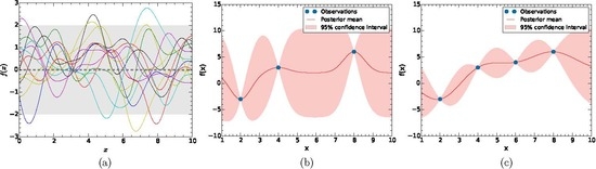
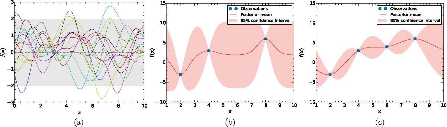
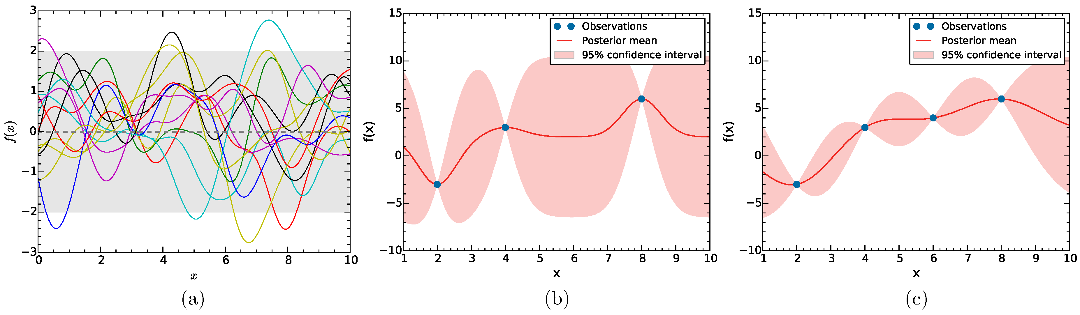
Given a set of observations (e.g., a typical light curve) with the form , where represent recorded flux densities at times , we would like to find all functions drawn from the prior distribution which pass through all observations. The latter distribution would be the posterior distribution, and its mean value describes the data best (see Figure 1).
What generates the prior distribution is a covariance kernel or function. This governs the similarity (covariance) between any two function values—e.g., at and . It is chosen based on our prior knowledge regarding the system. There exists a multitude of kernels which can model unknown functions based on their characteristics (e.g., periodic, linear, etc.) [20]. It is noteworthy that sums and products of kernels also produce valid kernels. For the purposes of this paper, the squared-exponential (SE) kernel is chosen. This is the simplest kernel, and the only underlying assumption is that of a smooth process (i.e., the functions it produces have derivatives of all orders everywhere in their domain). The SE kernel is defined as
with l the characteristic length scale (i.e., the distance in the x dimension after which the function changes significantly) and the variance (i.e., the mean distance of the function from its mean—serves only as a scaling factor). Here, l and are the hyperparameters.
2.2. Training the Gaussian Process
Bayesian model selection provides the way for optimizing the hyperparameters, thereby refining the posterior distribution and enabling us to perform inference. We essentially update our prior knowledge in the light of a data set. This is done by means of maximizing the log marginal likelihood [12], as outlined below.
For the SE kernel, the vector of hyperparameters is and the probability (or evidence) of the training data given the hyperparameters vector θ is . The log marginal likelihood is given by
More generally, in the case of a hyperparameter vector , the derivatives of the log marginal likelihood with respect to each are
3. Application to the Light Curves of the Blazar PKS 1502+106
PKS 1502+106 (S3 1502+10, OR 103) is a powerful flat-spectrum radio quasar (FSRQ), driven by a supermassive black hole of about M, at redshift (see Ref. [21] and references therein). The source was detected by Fermi in 2008, showing an intense γ-ray outburst at MeV–GeV energies [22]. The flare was monitored by F-GAMMA and other programs in the radio band. Radio data from the F-GAMMA program1 were employed, including observations with the Effelsberg 100-m (EB) and the IRAM 30-m (PV) telescopes in ten frequency bands from 2.64 to 142.33 GHz. Monthly observations from the EB and PV telescopes were performed quasi-simultaneously, thus ensuring maximum spectral coherency. A detailed description of the observational setup and data reduction is provided elsewhere [7,10,23,24].
Considering the full length of available multi-frequency light curves, GP regression was applied to the data at each frequency separately. A variant of the software presented in Ref. [25] was used, which was adapted to our specific modelling needs. A suite of machine learning applications for Python, including GP regression, is available online2.
To obtain the best unbiased result, the length scale parameter l was randomly initialized 100 times. Then, the posterior mean is returned with a 95% confidence interval for the flux density, along with the set of hyperparameters which maximize the log marginal likelihood. The relevant light curve parameters extracted are the peak amplitude (), the time of the peak, and the cross-band delay. Furthermore, the flare rise and decay times are calculated between the peak and the two flux density minima, which immediately precede and follow [18].
4. Results and Discussion
4.1. Quantifying the Broadband Outburst of PKS 1502+106
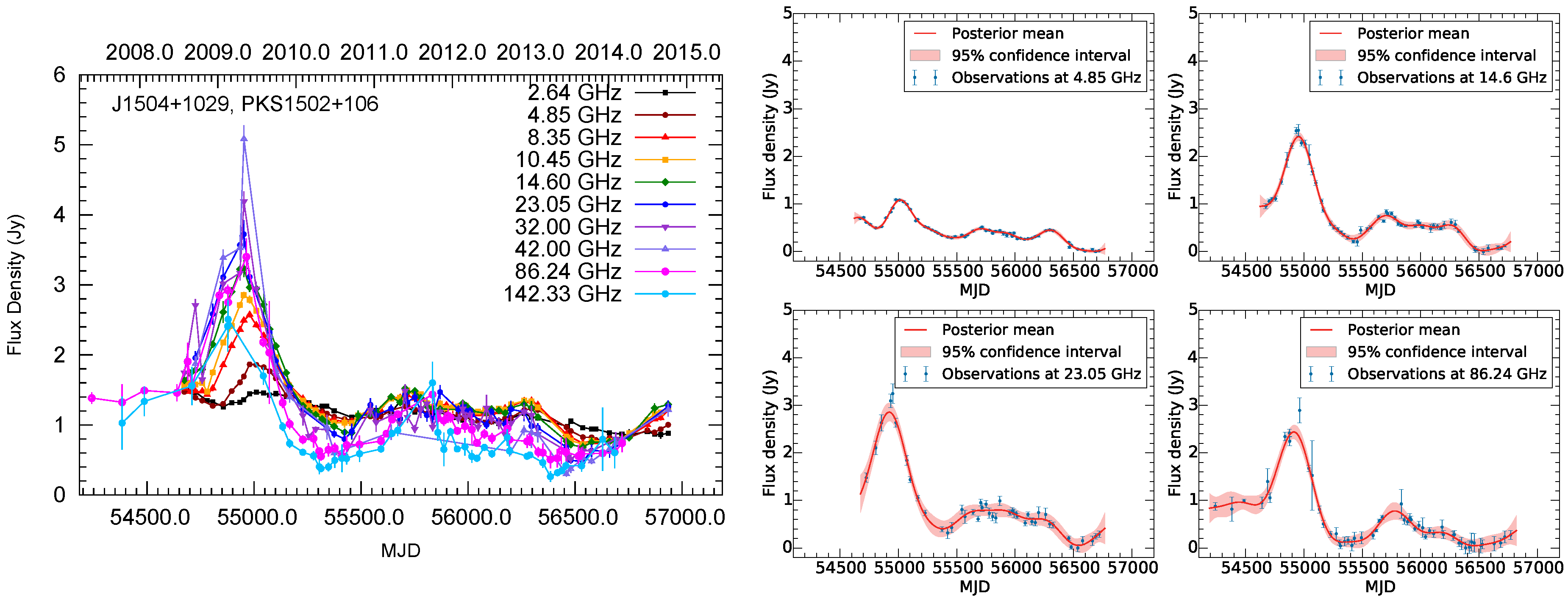
PKS 1502+106 has shown an isolated outburst visible across the electromagnetic spectrum. The results of the GP regression are visible in the right panels of Figure 2. The amplitudes at each of our radio frequencies first increase up to about 43 GHz, where they peak and then drop at higher ν (Figure 4 of Ref. [18]). The flare peaks with increasing time delay as we follow it towards lower frequencies (Figure 5 of Ref. [18]). The dependence of amplitudes and delays on ν can be well approximated by power laws—a telltale sign of shock evolution within the source’s parsec-scale jet. These results are in agreement with the study of the source using mm-wave very-long-baseline interferometry (mm-VLBI; see Ref. [21]).
The observed time lags between radio frequencies can be attributed to synchrotron opacity effects. In this context, the flare maxima appear first at higher frequencies and gradually progress to lower frequencies (e.g., Ref. [2]). Timing the flare maximum at each frequency with respect to the data at 142.33 GHz yields the following delays. The longest delay of days is seen between and GHz. Decreasing lags are clearly visible towards higher frequencies with a time lag of d at 4.85 GHz and d at 8.35 GHz. At higher frequencies, the lags are d at 10.45 GHz, d at 14.6, d at 23.03, and d at 32 GHz. At the two highest frequencies of 43.05 GHz and 86.24 GHz, the lags are d and d, respectively (see Table 3 of Ref. [18]).
The aforementioned lags allow the calculation of the synchrotron opacity profile of PKS 1502+106. Considering that at a given frequency the core represents a feature whose optical depth is close to unity, the standard relativistic jet paradigm predicts that the apparent position of this unit-opacity surface depends on observing frequency (see Ref. [18] and references therein). The importance of this “core-shift” effect lies in the fact that it gives critical insights into the physical processes of ultracompact jets, like the de-projected distance between the core (at each frequency) and the jet base, as well as the strength of the magnetic field along the flow (e.g., Refs. [26,27]). Using a “time-lag core shift” method—which proves to be a good alternative to VLBI core-shifts (e.g., Refs. [9,28])—the positions of the nine unit-opacity surfaces (or photospheres) with respect to the jet base were inferred. These are: pc for the 2.64 GHz core, pc at 4.85, pc at 8.35, pc at 10.45, pc at 14.60, pc at 23.05, pc at 32.00, pc at 43.05, and pc at 86.24 GHz (see Table 4 of Ref. [18] for the values and their calculation). Finally, we obtain the equipartition magnetic field along the jet axis, with values increasing from 14 mG at the 2.64 GHz core up to 176 mG at 86.24 GHz.
4.2. Where Do the γ Rays Come from?
The location of the γ-ray-emitting region is decisively constrained by combining the aforementioned findings with those of Refs. [23] and [21]. Specifically, in Ref. [23], the authors calculate the relative distance between the 86 GHz core and the γ-ray site to be about 2.1 pc, while in Ref. [21], using high-resolution mm-VLBI imaging, the knot most likely connected with the flare in question is identified (knot C3) and its kinematical properties are deduced ( c, jet viewing angle of ).
Having calculated the absolute distance between the jet base and the 86.24 GHz core pc, and with the relative separation between the same core and the γ-ray site (2.1 pc), the high-energy emission originates at pc from the jet base. This places it far from the bulk of the broad-line material of the source ( pc), making external Compton—on a field other than that of the BLR—a very relevant emission mechanism for PKS 1502+106’s γ ray emission, with significant implications on the origin of the seed photon field (see Ref. [18] and references therein).
Acknowledgments
V.K. thanks Lars Fuhrmann, Emmanouil Angelakis, Thomas P. Krichbaum, Ioannis Myserlis, Ioannis Nestoras, J. Anton Zensus, and Hans Ungerechts for interesting discussions and useful comments; also Walter Max-Moerbeck and B. Boccardi for carefully reading the paper. Partially based on observations with the Effelsberg 100-m and the IRAM 30-m telescopes.
Conflicts of Interest
The author declares no conflict of interest.
References
- Marscher, A.P.; Gear, W.K. Models for high-frequency radio outbursts in extragalactic sources, with application to the early 1983 millimeter-to-infrared flare of 3C 273. Astrophys. J. 1985, 298, 114–127. [Google Scholar] [CrossRef]
- Valtaoja, E.; Terasranta, H.; Urpo, S.; Nesterov, N.S.; Lainela, M.; Valtonen, M. Five Years Monitoring of Extragalactic Radio Sources—Part Three—Generalized Shock Models and the Dependence of Variability on Frequency. Astron. Astrophys. 1992, 254, 71. [Google Scholar]
- Spada, M.; Ghisellini, G.; Lazzati, D.; Celotti, A. Internal shocks in the jets of radio-loud quasars. Mon. Not. R. Astron. Soc. 2001, 325, 1559–1570. [Google Scholar] [CrossRef]
- Camenzind, M.; Krockenberger, M. The lighthouse effect of relativistic jets in blazars—A geometric origin of intraday variability. Astron. Astrophys. 1992, 255, 59–62. [Google Scholar]
- Fuhrmann, L.; Zensus, J.A.; Krichbaum, T.P.; Angelakis, E.; Readhead, A.C.S. Simultaneous Radio to (Sub-) mm-Monitoring of Variability and Spectral Shape Evolution of potential GLAST Blazars. In Proceedings of the First GLAST Symposium, Stanford, CA, USA, 5–8 February 2007; Ritz, S., Michelson, P., Meegan, C.A., Eds.; American Institute of Physics: Melville, NY, USA, 2007; Volume 921, pp. 249–251. [Google Scholar]
- Angelakis, E.; Fuhrmann, L.; Nestoras, I.; Zensus, J.A.; Marchili, N.; Pavlidou, V.; Krichbaum, T.P. The F-GAMMA program: Multi-wavelength AGN studies in the Fermi-GST era. arXiv, 2010; arXiv:1006.5610. [Google Scholar]
- Fuhrmann, L.; Angelakis, E.; Zensus, J.A.; Nestoras, I.; Marchili, N.; Pavlidou, V.; Karamanavis, V.; Ungerechts, H.; Krichbaum, T.P.; Larsson, S.; et al. The F-GAMMA program: Multi-frequency study of Active Galactic Nuclei in the Fermi era. Program description and the first 2.5 years of monitoring. arXiv, 2016; arXiv:1608.02580. [Google Scholar]
- Valtaoja, E.; Lähteenmäki, A.; Teräsranta, H.; Lainela, M. Total Flux Density Variations in Extragalactic Radio Sources. I. Decomposition of Variations into Exponential Flares. Astrophys. J. Suppl. 1999, 120, 95–99. [Google Scholar] [CrossRef]
- Kudryavtseva, N.A.; Gabuzda, D.C.; Aller, M.F.; Aller, H.D. A new method for estimating frequency- dependent core shifts in active galactic nucleus jets. Mon. Not. Roy. Astron. Soc. 2011, 415, 1631–1637. [Google Scholar] [CrossRef]
- Angelakis, E.; Fuhrmann, L.; Marchili, N.; Foschini, L.; Myserlis, I.; Karamanavis, V.; Komossa, S.; Blinov, D.; Krichbaum, T.P.; Sievers, A.; et al. Radio jet emission from GeV-emitting narrow-line Seyfert 1 galaxies. Astron. Astrophys. 2015, 575, A55. [Google Scholar] [CrossRef]
- Karamanavis, V. Zooming into γ-Ray Loud Galactic Nuclei: Broadband Emission and Structure Dynamics of the Blazar PKS 1502+106 and the Narrow-Line Seyfert 1 1H 0323+342. Ph.D. Thesis, Universität zu Köln, Cologne, Germany, 2015. [Google Scholar]
- Williams, C.K.I.; Rasmussen, C.E. Gaussian Processes for Regression. In Advances in Neural Information Processing Systems 8; MIT Press: Cambridge, MA, USA, 1996; pp. 514–520. [Google Scholar]
- Roberts, S.; Osborne, M.; Ebden, M.; Reece, S.; Gibson, N.; Aigrain, S. Gaussian processes for time-series modelling. Philos. Trans. R. Soc. Lond. A Math. Phys. Eng. Sci. 2012, 371, 20110550. [Google Scholar] [CrossRef] [PubMed]
- Ghahramani, Z. Probabilistic machine learning and artificial intelligence. Nature 2015, 521, 452–459. [Google Scholar] [CrossRef] [PubMed]
- Gibson, N.P.; Aigrain, S.; Roberts, S.; Evans, T.M.; Osborne, M.; Pont, F. A Gaussian process framework for modelling instrumental systematics: Application to transmission spectroscopy. Mon. Not. R. Astron. Soc. 2012, 419, 2683–2694. [Google Scholar] [CrossRef]
- Aigrain, S.; Pont, F.; Zucker, S. A simple method to estimate radial velocity variations due to stellar activity using photometry. Mon. Not. R. Astron. Soc. 2012, 419, 3147–3158. [Google Scholar] [CrossRef]
- Rajpaul, V.; Aigrain, S.; Osborne, M.A.; Reece, S.; Roberts, S. A Gaussian process framework for modelling stellar activity signals in radial velocity data. Mon. Not. R. Astron. Soc. 2015, 452, 2269–2291. [Google Scholar] [CrossRef]
- Karamanavis, V.; Fuhrmann, L.; Angelakis, E.; Nestoras, I.; Myserlis, I.; Krichbaum, T.P.; Zensus, J.A.; Ungerechts, H.; Sievers, A.; Gurwell, M.A. What can the 2008/10 broadband flare of PKS 1502+106 tell us? Nuclear opacity, magnetic fields, and the location of γ rays. Astron. Astrophys. 2016, 590, A48. [Google Scholar] [CrossRef]
- Rasmussen, C.E.; Williams, C.K.I. Gaussian Processes for Machine Learning (Adaptive Computation and Machine Learning); The MIT Press: Cambridge, MA, USA, 2005. [Google Scholar]
- Duvenaud, D. Automatic Model Construction with Gaussian Processes. Ph.D. Thesis, University of Cambridge, Cambridge, UK, 2014. [Google Scholar]
- Karamanavis, V.; Fuhrmann, L.; Krichbaum, T.P.; Angelakis, E.; Hodgson, J.; Nestoras, I.; Myserlis, I.; Zensus, J.A.; Sievers, A.; Ciprini, S. PKS 1502+106: A high-redshift Fermi blazar at extreme angular resolution. Structural dynamics with VLBI imaging up to 86 GHz. Astron. Astrophys. 2016, 586, A60. [Google Scholar] [CrossRef]
- Abdo, A.A.; Ackermann, M.; Ajello, M.; Atwood, W.B.; Axelsson, M.; Baldini, L.; Ballet, J.; Barbiellini, G.; Bastieri, D.; Baughman, B.M.; et al. PKS 1502+106: A New and Distant Gamma-ray Blazar in Outburst Discovered by the Fermi Large Area Telescope. Astrophys. J. 2010, 710, 810–827. [Google Scholar] [CrossRef]
- Fuhrmann, L.; Larsson, S.; Chiang, J.; Angelakis, E.; Zensus, J.A.; Nestoras, I.; Krichbaum, T.P.; Ungerechts, H.; Sievers, A.; Pavlidou, V.; et al. Detection of significant cm to sub-mm band radio and γ-ray correlated variability in Fermi bright blazars. Mon. Not. R. Astron. Soc. 2014, 441, 1899–1909. [Google Scholar] [CrossRef]
- Nestoras, I.; et al. F-GAMMA program: Multi-frequency study of Active Galactic Nuclei in the Fermi-GST era III. The first 5 years of IRAM 30-m monitoring. Astron. Astrophys. 2015. submitted. [Google Scholar]
- Pedregosa, F.; Varoquaux, G.; Gramfort, A.; Michel, V.; Thirion, B.; Grisel, O.; Blondel, M.; Prettenhofer, P.; Weiss, R.; Dubourg, V.; et al. Scikit-learn: Machine Learning in Python. J. Mach. Learn. Res. 2011, 12, 2825–2830. [Google Scholar]
- Lobanov, A.P. Ultracompact jets in active galactic nuclei. Astron. Astrophys. 1998, 330, 79–89. [Google Scholar]
- Hirotani, K. Kinetic Luminosity and Composition of Active Galactic Nuclei Jets. Astrophys. J. 2005, 619, 73–85. [Google Scholar] [CrossRef]
- Kutkin, A.M.; Sokolovsky, K.V.; Lisakov, M.M.; Kovalev, Y.Y.; Savolainen, T.; Voytsik, P.A.; Lobanov, A.P.; Aller, H.D.; Aller, M.F.; Lahteenmaki, A.; et al. The core shift effect in the blazar 3C 454.3. Mon. Not. R. Astron. Soc. 2014, 437, 3396–3404. [Google Scholar] [CrossRef]
Figure 1.
Gaussian process (GP) prior and posterior distributions: (a) Twenty randomly selected samples from the prior distribution, with zero mean and , using a squared exponential covariance kernel; (b) Regression results after training the GP with three error-free data points; (c) Same as in panel (b), but note the improved result with the addition of one more data point.

Figure 2.
Multi-wavelength light curves of PKS 1502+106. (Left) F-GAMMA light curves between 2.64 and 142.33 GHz; (Right) GP regression curves for the data at 4.85, 14.6, 23.05, and 86.24 GHz. For the results at all frequencies, see Ref. [18].
Figure 2.
Multi-wavelength light curves of PKS 1502+106. (Left) F-GAMMA light curves between 2.64 and 142.33 GHz; (Right) GP regression curves for the data at 4.85, 14.6, 23.05, and 86.24 GHz. For the results at all frequencies, see Ref. [18].

© 2017 by the author. Licensee MDPI, Basel, Switzerland. This article is an open access article distributed under the terms and conditions of the Creative Commons Attribution (CC BY) license ( http://creativecommons.org/licenses/by/4.0/).
Share and Cite
MDPI and ACS Style
Karamanavis, V. Gaussian Processes for Blazar Variability Studies. Galaxies 2017, 5, 19. https://doi.org/10.3390/galaxies5010019
AMA Style
Karamanavis V. Gaussian Processes for Blazar Variability Studies. Galaxies. 2017; 5(1):19. https://doi.org/10.3390/galaxies5010019
Chicago/Turabian StyleKaramanavis, Vassilis. 2017. "Gaussian Processes for Blazar Variability Studies" Galaxies 5, no. 1: 19. https://doi.org/10.3390/galaxies5010019
Note that from the first issue of 2016, this journal uses article numbers instead of page numbers. See further details here.