
Exoplanet Predictions Based on Harmonic Orbit Resonances


1
Lockheed Martin, Solar and Astrophysics Laboratory, Org. A021S, Bldg. 252, 3251 Hanover St., Palo Alto, CA 94304, USA
2
Research Office for Complex Physical and Biological Systems, Mutschellenstr. 179, 8038 Zürich, Switzerland
*
Author to whom correspondence should be addressed.
Galaxies 2017, 5(4), 56; https://doi.org/10.3390/galaxies5040056
Submission received: 2 June 2017
/
Revised: 13 September 2017
/
Accepted: 13 September 2017
/
Published: 25 September 2017
Abstract
:The current exoplanet database includes 5454 confirmed and candidate planets observed with the Kepler mission. We find 932 planet pairs from which we extract distance and orbital period ratios. While earlier studies used a logarithmic spacing, which lacks a physical model, we employ here the theory of harmonic orbit resonances, which contains quantized ratios instead, to explain the observed planet distance ratios and to predict undetected exoplanets. We find that the most prevailing harmonic ratios are (2:1), (3:2), and (5:3) in 73% of the cases, while alternative harmonic ratios of (5:4), (4:3), (5:2), and (3:1) occur in the other 27% of the cases. Our orbital predictions include 171 exoplanets, 2 Jupiter moons, 1 Saturn moon, 3 Uranus moons, and 4 Neptune moons. The accuracy of the predicted planet distances amounts to a few percent, which fits the data significantly better than the logarithmic spacing. This information may be useful for targeted exoplanet searches with Kepler data and to estimate the number of live-carrying planets in habitable zones.
1. Introduction
Recent discoveries have amassed a current catalog of over 5000 exoplanets [1], which contains the names of the host stars, the semi-major axes, and the orbital periods of the associated exoplanets (see website: exoplanets.org). The unprecedented statistics of these orbital parameters allows us for the first time to determine whether the planets are distributed in random distances from the central star or in some systematic order, as is expected from physical models of harmonic resonance orbits [2,3]. A data analysis of statistical exoplanet databases therefore provides key information on the physical process of the formation of planetary systems, as well as on the number and statistical probability of planets that are located in habitable zones around stars.
The existence of orbital resonances in the solar system has been known for a long time (e.g., see reviews by [2,3]. A particular clean example is given by the three Galilean satellites of Jupiter (Io, Europa, and Ganymede), for which [4] demonstrated their long-term stability on the basis of celestial mechanics perturbation theory. Other examples are the gaps in the rings of Saturn, the resonances of asteroids with Jupiter (Trojans, Thule, Hilda, Griqua, and Kirkwood gaps), as well as the harmonic orbital periods of the planets in our solar system. Low harmonic (integer) numbers of orbital periods warrant frequent conjunction times, which translates into frequent gravitational interactions that can stabilize a three-body system of planets (or asteroids). The stability of orbital resonances has been explained in terms of the libration of coupled pendulum systems [5]. Physical descriptions of celestial resonance phenomena are reviewed by [2,3].
Empirical models of planet distances, such as the Titius-Bode law or the generalized Titius-Bode law (with logarithmic spacing), are not consistent with harmonic orbit ratios and lack a physical model [6]. It is therefore imperative not to use such empirical laws for the prediction of exoplanets, but rather use physical models based on harmonic orbital resonances, which we pursue in this study. The notion of missing planets, which can be either undetected or non-existing objects, dates back a century [7,8]. Recent predictions of (missing) exoplanets are based on the original Titius-Bode law [9,10,11], the logarithmic spacing of the generalized Titius-Bode law [12,13,14], an exponential function [15,16,17], or a multi-modal probability distribution function [18]. A recent study analyzed the statistical distribution of mean-motion resonances and near-resonances in 1176 exoplanet systems, finding a preference for (3:2) and (2:1) resonances in the overall, but large variations of the harmonic ratio for different planet types, grouped by their semi-major axis size, their mass, or their host-star type [19]. Most recently, a harmonic orbit resonance model with five dominant harmonic ratios (3:2, 5:3, 2:1, 5:2, and 3:1) was found to fit the observed orbital periods and distances of the planets and moons in our solar system, as well as in two exoplanet systems [6].
Orbital resonances can cause both instability and long-term stability. There are three general types of resonance phenomena in the solar system that involve orbital motions: (i) spin-orbit resonance (a commensurability of the period of rotation of a satellite with the period of its orbital reovlution), (ii) secular resonance (a commensurability of the frequencies of precession of the orientation of orbits), and (iii) mean-motion resonance (the most obvious type of resonance in a planetary system that occurs when the orbital periods of two bodies are close to a ratio of small integers) [2]. Here, we model the present (supposedly long-term and stable) configuration of the solar system, but we would expect that the planets’ configuration and their harmonic ratios may have changed in the past, especially during the heavy bombardment of lunar rocks 4 Gyrs ago, supposedly triggered by the rapid migration of the giant planets as the result of a destabilization [20,21,22].
In this study, we identify a set of dominant harmonic ratios that fit the observed exoplanet orbital period ratios, and infer the statistical probability of these best-fit harmonic ratios. On the basis of this analysis, we present predictions of so far undetected exoplanets in 190 exoplanet systems. We describe the data analysis method and the observational results in Section 2, which are followed by the discussion and conclusions in Section 3.
2. Observations and Data Analysis Method
2.1. Data Set Statistics
We accessed the web-based exoplanet database http://exoplanets.org and found at the time of this analysis (10 May 2017) a total of 5454 detected exoplanets, which included confirmed planets as well as candidate planets from the Kepler mission. Most of the exoplanets represented single detections in a star system, which applied for 3860 cases. Double-planet detections occurred in 472 star systems, triple-planet systems in 128, quadruple-planet systems in 44, quintuple-planet systems in 14, and sextuple-planet systems in 2. The largest planet systems had seven detections of planets, such as the KIC-11442793 and the TRAPPIST-1 systems [23]. We updated the TRAPPIST-1 system, with three stars given in the exoplanet database, to seven stars, as given by [23] and analyzed also by [24,25]. All these exoplanet detections were associated with a total of 4522 different stars (Table 1).
For our analysis, we were most interested in studying harmonic resonance orbit ratios, requiring at least two neighbored exoplanets per star, which amounted to a total of 622 exoplanets, or 932 planet pairs. We also attempted to find predictions of missing planets, which required at least three planets per star (yielding a comparison between at least two harmonic ratios) and which was feasible in 190 exoplanet systems.
2.2. Orbital Period Ratio Distribution
An important result of our analysis is the distribution of orbital period ratios , where and are the orbital time periods in a planetary system with planets. These orbital periods are directly related to the semi-major axis D of the planets, according to Kepler’s third law (using the units of AU and years):
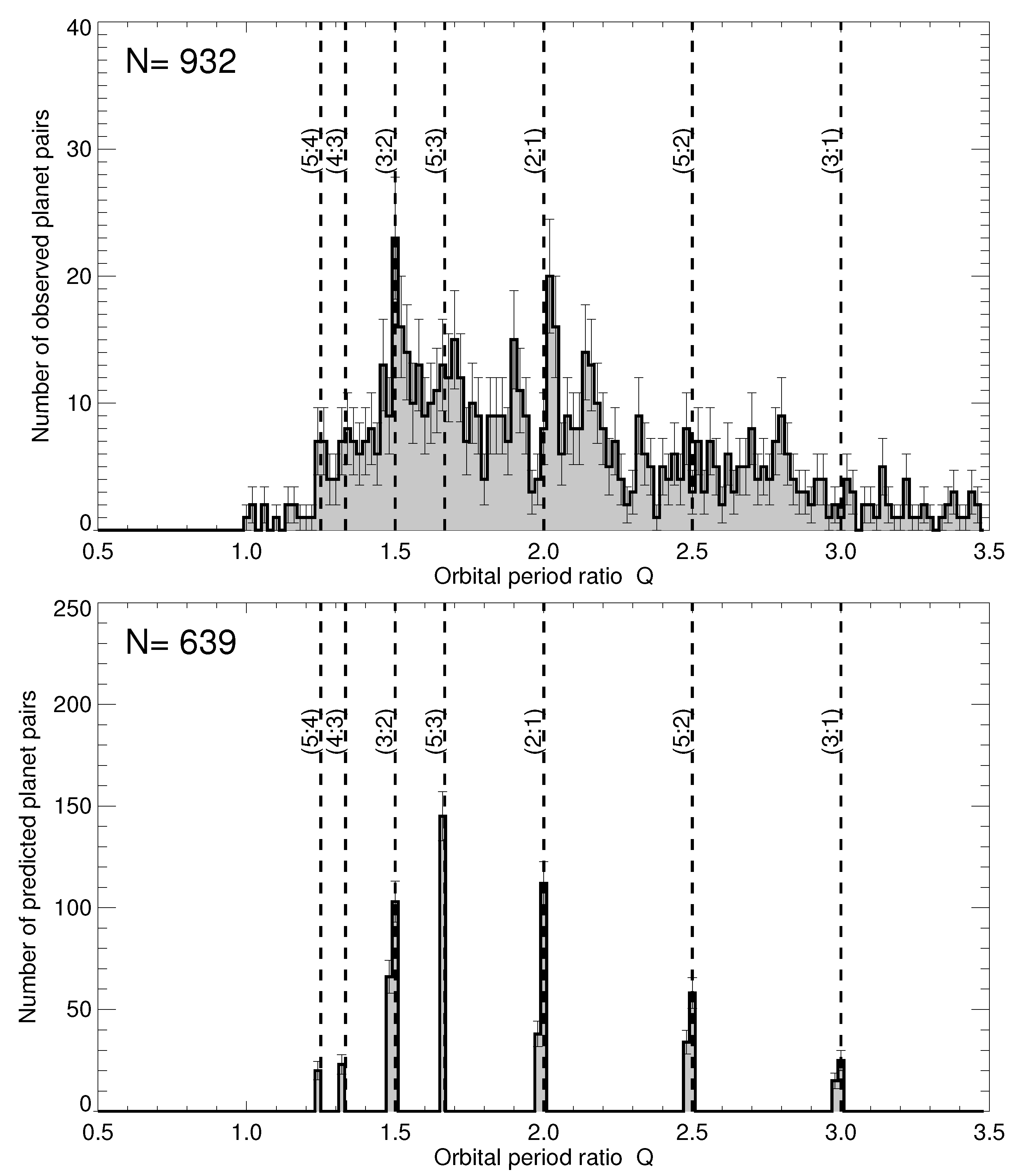
We have plotted a histogram of orbital period ratios for all planet pairs in Figure 1 (top panel), sampled in a range of with a histogram bin width of . These period ratios Q are defined from the ratios of the outer planet orbital period to the inner planet orbital period , which is always larger than unity by definition, that is, , because the inner planets rotate faster around the Sun than the outer planets. We added error bars in Figure 1 (top panel), with denoting the number of values per bin, as expected from Poisson statistics.
What is striking about the period distribution shown in Figure 1 (top panel) is that the periods do not follow a smooth (approximately log-normal) distribution, but rather exhibit significant peaks at the harmonic values of Q = (3:2) = 1.5 and at P = (2:1) = 2.0, which involve the strongest harmonic resonances, associated with the lowest harmonic numbers 1, 2, and 3. In a previous study on our own solar system and on the moons around planets, we noticed the dominance of five low harmonic ratios, that is, (3:2), (5:3), (2:1), (5:2) and (3:1) [6]. Interestingly, we find now (top of Figure 1) that exoplanets confirm the preponderance of harmonic ratios (3:2), (2:1) and (5:3), while the other ratios, (3:1) and (5:2), are less significant.
The distribution of harmonic ratios drops steeply from towards a value of at the low side, while the upper end extends all the way to . The extended tail at the upper end can be explained by a large number of missing (undetected) planets, for which the most extreme ratio applies to the case in which only the innermost and the outermost planet are detected. For our solar system, this maximum ratio would be the orbital period ratio between Mercury and Pluto, that is, = 248 years/0.24 years ≈ 1033.
2.3. Orbital Period Ratios of Large Planet Systems
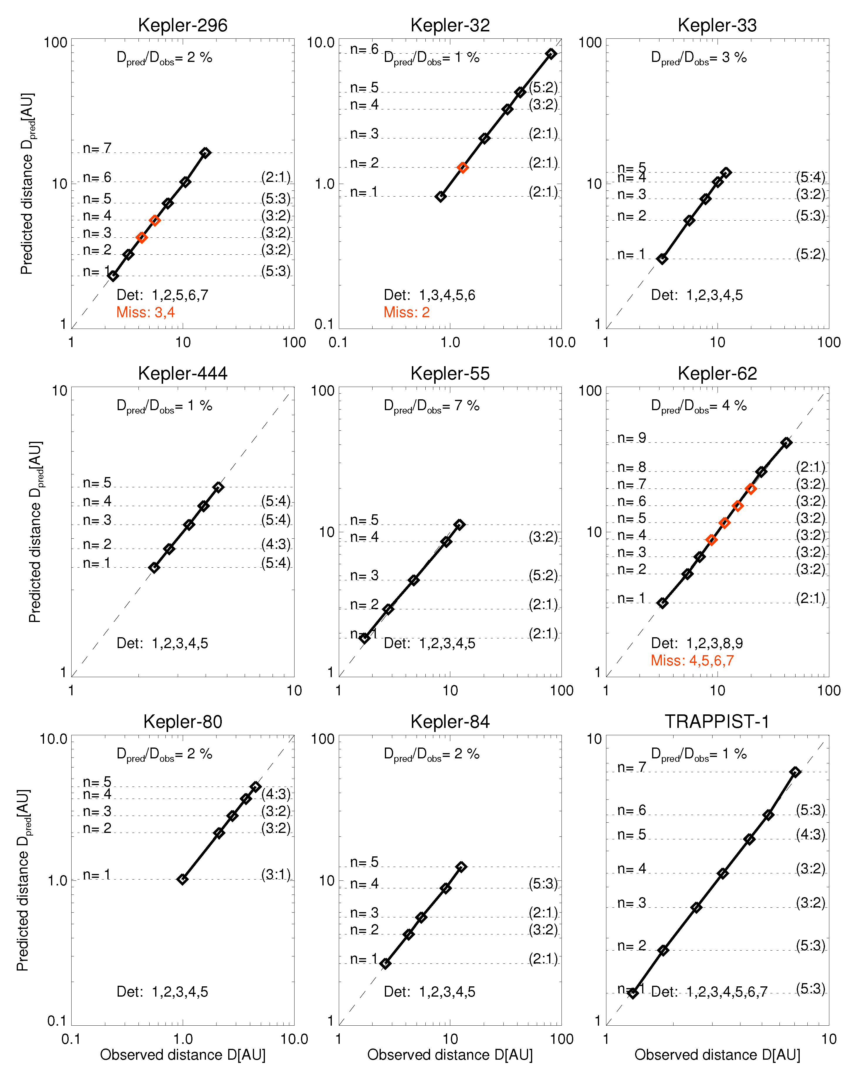
In Figure 2 and Figure 3, we show the orbital distances D for the 18 largest exoplanet systems (in alphabetical order), which include all the cases with 5, 6, or 7 planets per star. Each panel in Figure 2 and Figure 3 displays the best-fit planet distances (from the central star) to the observed planet distances. While we quote harmonic ratios of the orbital periods throughout the paper, the corresponding distances (as shown in Figure 2 and Figure 3) are simply calculated from Kepler’s third law (Equation (1)). If we limit ourselves to a maximum orbit ratio of , we find that all observed orbital period ratios in this subset (shown in Figure 2 and Figure 3) can be explained by seven harmonic ratios (with small harmonic numbers) in the range of (5:4) = 1.25, (4:3) = 1.333, (3:2) = 1.5, (5:3) = 1.667, (2:1) = 2.0, (5:2) = 2.5, and (3:1) = 3.0, which we define as “principal harmonic ratios”. From the largest 18 systems shown in Figure 2 and Figure 3, we find that half of them are “gap-free exoplanet systems”, which means that all detected period ratios can be explained with these principal harmonic ratios in the range of 1.25 3.0, such as Kepler-11, Kepler-154, Kepler-292, Kepler-33, Kepler-444, Kepler-55, Kepler-80, Kepler-84, and TRAPPIST-1. In all other cases, we find some “gaps”, which are manifested by orbital period ratios of . These gaps are likely to be produced by missing (undetected) planets (marked with red diamonds in Figure 2 and Figure 3), such as 55-Cnc, HD-10180, KIC-11442793, Kepler-169, Kepler-186, Kepler-20, Kepler-296, Kepler-32, and Kepler-62. Because the largest exoplanet systems have 7 members so far, while our own solar system hosts 10 planetary objects (i.e., 8 true planets as well as Pluto and the asteroid belt), it is likely that there are more missing exoplanets outside the so far detected gap-free sequences.
2.4. Strategy for Predicting Missing Exoplanets
Previous studies developed strategies to predict missing (undetected or non-existing) exoplanets from the generalized Titius-Bode law, which assumes a constant geometric progression factor Q, that is, (e.g., [12]). In a recent study, however, we found that the observational data support quantized harmonic resonance ratios, such as [6], rather than a constant progression factor Q. Such a quantization thus has to be included in a search strategy for missing (undetected) exoplanets. On the other hand, the generalized Titius-Bode law is simpler to fit to data, because it is controlled by a single free parameter Q, while fitting a harmonic resonance model is more ambiguous because of a larger number of quantized parameters .
Our approach is to reduce the n-body problem to a special three-body problem with a pair of two satellites (with masses and ) orbiting a much heavier star (with mass ), assuming that they have achieved a long-term stability of their orbits (otherwise they would not be observable), which is most likely accomplished by mechanical resonances and manifests itself by low harmonic ratios of the their orbital periods. In this simple model, we neglect the masses and resulting gravitational disturbances from additional planets. In the case of undetected planets, perturbations of observed planets could lead to predictions of the orbits and masses of undetected planets, such as was accomplished with the discovery of the outer planets (Uranus, Neptune, and Pluto).
The problem can be formulated as an optimization problem of predicting a gap-free sequence of harmonic ratios:
where the orbital period ratios are drawn from the range of principal harmonic ratios in such a way that the observed subset of orbital periods of the detected exoplanets matches the best-fit periods .
In the following, we develop a search strategy that is consistent with harmonic resonance orbits and that consists of the following steps: (1) We define a range of seven principal low harmonics: (5:4) = 1.25, (4:3) = 1.333, (3:2) = 1.5, (5:3) = 1.667, (2:1) = 2.0, (5:2) = 2.5, and (3:1) = 3.0. Neighbored exoplanet orbit pairs with ratios in the range of 1.13.1 are attributed to the closest principal harmonic ratio. (2) Orbital ratios in the range of 1.0 1.1 are interpreted as planet pairs in identical harmonic resonance zones, which are found only for very small bodies (such as asteroids or moons of Jupiter and Saturn with diameters of km). (3) Detected planet pairs with orbital periods of Q3.1 are interpreted as gaps with one or more missing (undetected) planets. Because a gap has to be filled by planets, that is, ≈ , we determine the number of missing planets from the observed ratio = / by
where Round represents a rounding function to the next integer number. The characteristic ratio is estimated from the best-fitting value of the five most frequent principal harmonic ratios, that is, = 1.5, 1.667, 2.0, 2.5, and 3.0. The best-fitting value is simply determined by minimizing the mean deviation between the observed () and the best-fit () orbital periods:
which translates into a mean deviation of planet distances D according to Kepler’s law (Equation (1)):
An additional constraint is the estimated maximum number of planets per system, which we choose to be on the basis of the number of planets detected in our solar system ( including Pluto and the asteroids) and the number of Jupiter’s moons () or Saturn’s moons () that fit the scheme (see Appendix A for our solar system and planetary moon systems).
These best-fit mean deviations are listed in the 18 panels in Figure 2 and Figure 3. We see that these best-fit solutions of harmonic ratios match the observed orbital period ratios typically within an accuracy of ≈1–5%. The most accurate harmonic ratios with an accuracy of ≈1% are found for the planetary systems of Kepler-169, Kepler-32, Kepler-444, and TRAPPIST-1.
Certainly, the estimated missing planets bear some ambiguity, because the ratios in subsequent intervals in a gap can be permutated arbitrarily. For instance, if we take out a planet between two resonance zones of = (3:2) and = (2:0), the permutated sequence = (2:0) and = (3:2) yields an identical solution, and thus the predicted resonance at the location of the filled gap is only accurate to /, which is attributed to the closest admissible resonance ratio of (5:3) = 1.667 and which yields a combined period ratio of (5:3) × (5:3) = 2.778 in the gap; this is within 8% of the correct gap value, (3:2) × (2:1) = 3.0.
2.5. Statistical Probability of Quantized Periods
After we corrected each detected exoplanet sequence of orbital periods per exoplanet system or star (for exoplanet systems with more than three detected exoplanets), by predicting missing exoplanet detections according to the algorithm described above, we could sample the distribution of predicted orbital periods, as is shown in Figure 1 (bottom panel). The predicted distribution of orbital period ratios was then, as a consequence of the applied prediction scheme, quantized according to the seven principal harmonic ratios, while no ratio was found outside the range of . What this quantized distribution reveals, moreover, is the statistical probability for the individual harmonic ratios. According to the result shown in Figure 1 (bottom panel), the highest probability exists for the harmonic ratios of (3:2), (5:3) and (2:1), while the other four harmonic ratios are significantly rarer. The relative probabilities for each of the seven principal harmonic ratios are as follows (in the order of decreasing probability): 26% for a ratio of (3:2), 25% for a ratio of (2:1), 22% for a ratio of (5:3), 14% for a ratio of (5:2), 6% for a ratio of (3:1), 4% for a ratio of (4:3), and 3% for a ratio of (5:4).
2.6. Catalog of Exoplanet Predictions
In Table 2, we list the planet distances of all 190 exoplanet systems with more than 3 planets. The observed period ratios of the 190 exoplanet systems amount to a total of values (see statistics in Table 1). The number of predicted exoplanets for this sample are marked with parentheses in Table 2, amounting to a total of 171 predictions. These predicted distances of undetected exoplanets can be used in targeted searches with Kepler data or other data.
3. Discussion and Conclusions
The knowledge of planet distances from their host star provides us with several important pieces of information. One central insight that can only be proven with reliable planet distance ratios is the physical formation process of planetary systems. A leading theory in this respect is the harmonic orbit resonance concept, which implies that multiple planets entrain into long-term stable orbits only once their orbits approach a harmonic ratio with low numbers. Our analysis of 932 exoplanet pairs yielded evidence that the prevailing harmonic ratios are (2:1), (3:2), and (5:3), which dominate in 73% of all exoplanet pairs and which is consistent with the finding of [19], while less additional harmonic ratios of (5:4), (4:3), (5:2), and (3:1) also occur, but are less frequent (in 27% of all cases). This relative probability of harmonic ratios in planet orbits is a quantitative result that can be tested with numerical simulations of n-body gravitational perturbation theory.
What is the predictive power of this exercise for missing exoplanets? Previous studies employed the generalized Titius-Bode law (e.g., [12]), which assumes a constant geometric progression factor (or orbit-period progression factor Q by applying Kepler’s third law), also called logarithmic spacing. A constant progression factor has mostly been used for the sake of mathematical simplicity because it has only one free parameter, but it has no physical justification and is inconsistent with harmonic orbital resonance theories, which predict quantized values of low harmonic-number ratios, such as our set of seven principal harmonic numbers. However, there are a few rare cases that are consistent with an almost constant progression factor, such as Q = (5:2) = 2.5 for 55-Cnc (Figure 2) or Q = (5:3) = 1.67 for Kepler-20 (Figure 2), for which the harmonic orbit resonance model degenerates to the generalized Titius-Bode law.
The prediction of missing planets requires an algorithm that is based on low harmonic-number ratios, which is more difficult to fit in the presence of gaps than a constant progression factor for logarithmic spacing. Consequently, in fitting a complete planet system without gaps (of missing undetected planets), each planet orbit period ratio has up to seven free parameters (corresponding to the principal low harmonic ratios). Although this creates some ambiguity, as the best solution is insensitive to permutations of interpolated orbit period ratios, we eliminated this ambiguity by minimizing the difference between the observed and modeled planet distances. In summary, the prediction of missing planets is based on solutions of orbital period sequences that contain harmonic-number ratios only, rather than a constant logarithmic spacing.
The term “missing planet” refers to either an undetected object or a non-existing object, which we cannot discriminate between at this stage, especially not with the two-body resonance ratios that are fitted here. If we would generalize the model to three-body resonances, the two interpretations could possibly be discriminated in some cases.
The orbital prediction of missing planets obtained here includes 2 Jupiter moons, 1 Saturn moon, 3 Uranus moons, 4 Neptune moons, and 171 exoplanets (Figure 2, Figure 3 and Figure 4 and Table 2). The accuracy of the predicted planet distances amounts to a few percent. A previous study has shown that the harmonic orbit resonance model with quantized values fits the solar system and lunar systems better than the assumption of uniform logarithmic spacing [6]. This information may be useful for targeted searches of exoplanets with Kepler data, as it reduces the search parameter space. Moreover, it allows us to estimate the number of habitable planets in each exoplanet system [26].
The existence of quantized values in planetary distances represents a system with (non-random) order, which falls into the category of self-organizing systems [6]. Self-organizing systems are characterized by regular geometric patterns that result from frequent local interactions in an initially disordered system (e.g., the libration of coupled pendulums). The principle of self-organization, however, should not be confused with the concept of self-organized criticality [27] in nonlinear dissipative systems, which is also common in astrophysics [28].
Acknowledgments
This research has made use of the Exoplanet Orbit Database and the Exoplanet Data Explorer at exoplanets.org. The first author acknowledges the hospitality and partial support for two workshops on “Self-Organized Criticality and Turbulence” at the International Space Science Institute (ISSI) in Bern, Switzerland, during 15–19 October 2012 and 16–20 September 2013, as well as constructive and stimulating discussions (in alphabetical order) with Sandra Chapman, Paul Charbonneau, Henrik Jeldtoft Jensen, Lucy McFadden, Maya Paczuski, Jens Juul Rasmussen, John Rundle, Loukas Vlahos, and Nick Watkins. This work was partially supported by NASA, contract NNX11A099G: “Self-organized criticality in solar physics”.
Author Contributions
M.J.A. performed the data analysis and wrote the paper. F.S. contributed information and previous data analysis of the TRAPPIST-1 exoplanet system.
Conflicts of Interest
The authors declare no conflict of interest.
Appendix A. Solar System and Planetary Moon Systems
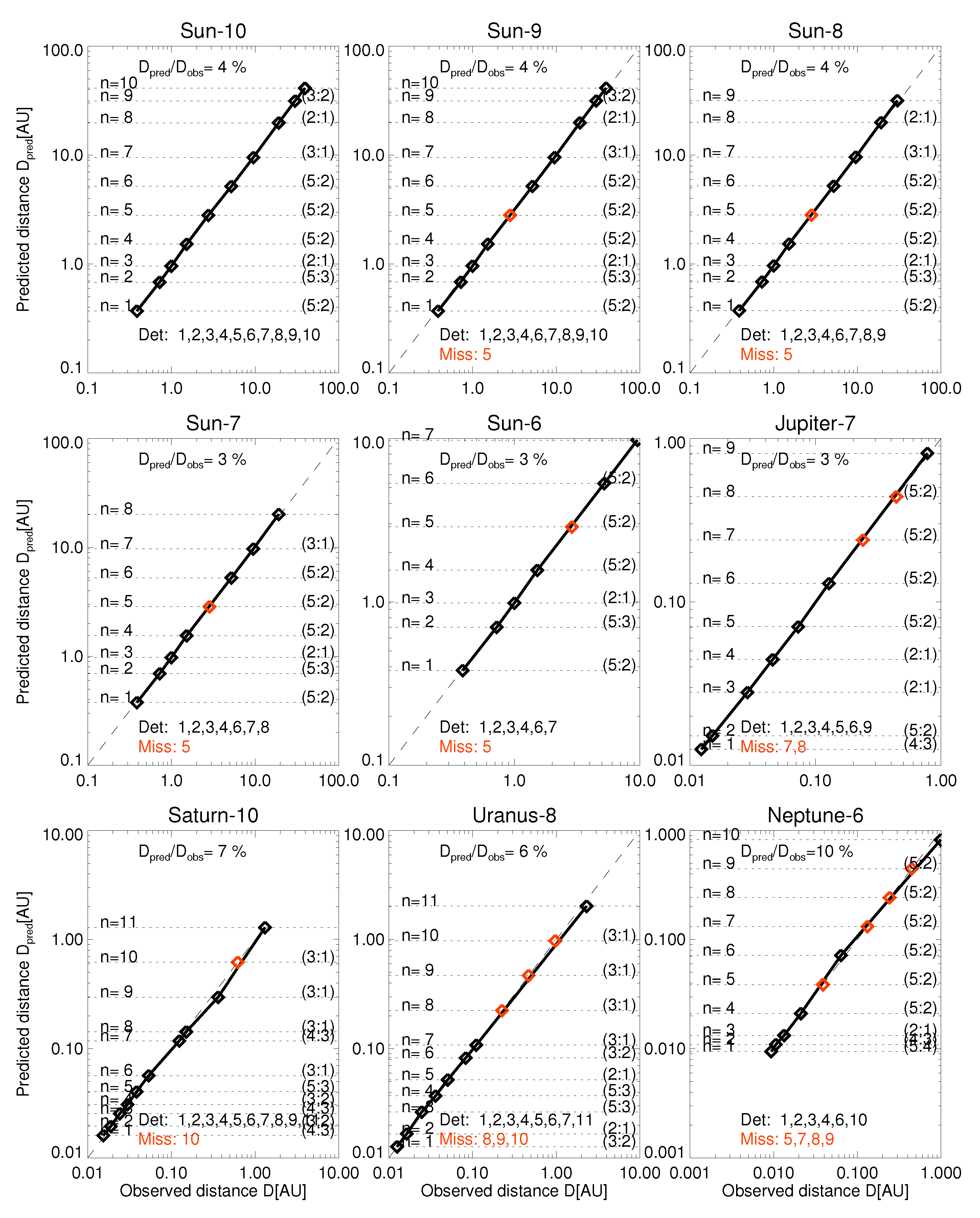
As a consistency test, we applied our prediction algorithm for missing exoplanets (Section 2.4) to our solar system and to the moon systems described in a previous study [6]. The results are shown in Figure 4.
First, we used the planet distances from Sun’s center for all 10 planetary objects of our solar system, including the asteroid Ceres, shown in the panel labeled as Sun-10. Because no harmonic ratio larger than (3:1) occurs, our algorithm predicted no missing planet. In the second panel (labeled as Sun-9) we eliminated the asteroid Ceres, which was then detected as a missing planet with our algorithm, because the harmonic ratio between Mars and Jupiter exhibits a ratio of ≈4.0 that is significantly larger than the largest admissible principal harmonic ratio of 3.0. In the panel Sun-8, we eliminated Pluto in addition, which mimicked the situation before 1930. In the panel Sun-7, we eliminated Neptune (before 1846), and in panel Sun-6 we eliminated Uranus (before 1781). In all four cases, Sun-9, Sun-8, Sun-7, and Sun-6, our algorithm consistently flagged only the asteroid Ceres, because in each situation, the outermost planet was removed, while the remaining planets represented a gap-free sequence.
In panel Jupiter-7 (in Figure 4), we sampled all Jupiter’s moons with a diameter of km, namely, Amalthea, Thebe, Io, Europa, Ganymede, Callisto and Himalia. Our algorithm predicted two missing moons between the two outermost detected moons Callisto and Himalia (similar to Figure 6 by [6]).
In panel Saturn-10 (in Figure 4), we sampled all Saturn’s moons with a diameter of km, namely, Janus, Mimas, Enceladus, Thetis, Dione, Rhea, Tian, Hyperion, Japetus, and Phoebe. Our algorithm predicted one missing moon between the two outermost detected moons Japetus and Phoebe (similar to Figure 7 by [6]).
In panel Uranus-8 (in Figure 4), we sampled all Uranus’ moons with a diameter of km, namely, Portia, Puck, Miranda, Ariel, Umbriel, Titania, Oberon, and Scycorax. Our algorithm predicted three missing moons between the two outermost detected moons Oberon and Scycorax (similar to Figure 8 by [6]).
In panel Neptune-6 (in Figure 4), we sampled all Neptune’s moons with a diameter of km, namely, Galatea, Despina, Larissa, Proteus, Proteus, Triton, and Nereid. Our algorithm predicted three missing moons between the two outermost detected moons Triton and Nereid, and one missing moon between Proteus and Triton (similar to Figure 9 by [6]).
Altogether, our harmonic resonance model with an upper limit of for the highest admissible harmonic number predicted a total of 10 missing moons in our own planetary system. We note that none of the predicted sequences exceeded a maximum of 11 moons per planetary system.
References
- Han, E.; Wang, S.; Wright, J.T.; Feng, Y.K.; Zhao, M.; Fakhouri, O.; Brown, J.I.; Hancock, C. Exoplanet Orbit Database. II. Updates to Exoplanets.org. Pubs. Astron. Soc. Pac. 2014, 126, 827. [Google Scholar] [CrossRef]
- Malhotra, R. Solar System Formation and Evolution; Lazarro, D., Vieira Martins, R., Ferraz-Mello, S., Fernandez, J., Eds.; Astronomical Society of the Pacific: California, CA, USA, 1998; Volume 149, p. 37. [Google Scholar]
- Peale, S.J. Orbital resonances in the solar system. Annu. Rev. Astron. Astrophys. 1976, 14, 215–246. [Google Scholar] [CrossRef]
- Laplace, P.S. Mécanique Céleste; Hillard, Gray, Little and Wilkins: Boston, MA, USA, 1829. [Google Scholar]
- Brown, E.W.; Shook, C.A. Planetary Theory; Dover: New York, NY, USA, 1933. [Google Scholar]
- Aschwanden, M.J. Self-organizing systems in planetary physics: harmonic resonances of planet and moon orbits. New Astron. 2018, 58, 107–123. [Google Scholar] [CrossRef]
- Armellini, G. Sopra le distanze dei pianeti dal Sole. Astr. Nachr. 1921, 215, 263–264. [Google Scholar] [CrossRef]
- Basano, L.; Hughes, D.W. A modified titius-bode law for planetary orbits. Il Nuovo Cimento 1979, 2, 505–510. [Google Scholar] [CrossRef]
- Cuntz, M. Application of the Titius–Bode Rule to the 55 Cancri System: Tentative Prediction of a Possibly Habitable Planet. Publ. Astron. Soc. Jpn. 2012, 64, 73. [Google Scholar] [CrossRef]
- Poveda, A.; Lara, P. Revista mexicana de astronomía y astrofísica. Rev. Mex. Astron. Astrofisica 2008, 44, 243–246. [Google Scholar]
- Qian, S.B.; Liu, L.; Liao, W.P.; Li, J.; Zhu, L.Y.; Dai, Z.B.; He, J.J.; Zhao, E.G.; Zhang, J.; Li, K. Detection of a planetary system orbiting the eclipsing polar HU Aqr. Mon. Not. R. Astron. Soc. 2011, 414, L16–L20. [Google Scholar] [CrossRef]
- Bovaird, T.; Lineweaver, C.H. Exoplanet predictions based on the generalized Titius-Bode relation. Mon. Not. R. Astron. Soc. 2013, 435, 1126–1138. [Google Scholar] [CrossRef]
- Bovaird, T.; Lineweaver, C.H.; Jacobsen, S.K. Using the inclinations of Kepler systems to prioritize new Titius–Bode-based exoplanet predictions. Mon. Not. R. Astron. Soc. 2015, 448, 3608–3627. [Google Scholar] [CrossRef]
- Huang, C.X.; Bakos, G.A. Testing the Titius–Bode law predictions for Kepler multiplanet systems. Mon. Not. R. Astron. Soc. 2014, 442, 674–681. [Google Scholar] [CrossRef]
- Lovis, C.; Segransan, D.; Mayor, M.; Udry, S.; Benz, W.; Bertaux, J.L.; Bouchy, F.; Correia, A.C.M.; Laskar, J.; Curto, G.L. The HARPS search for southern extra-solar planets-XXVIII. Up to seven planets orbiting HD 10180: probing the architecture of low-mass planetary systems. Astron. Astrophys. 2011, 528, A112. [Google Scholar] [CrossRef]
- Pletser, V. Exponential distance laws for satellite systems. Earth Moon Planets 1986, 36, 193–210. [Google Scholar] [CrossRef]
- Pletser, V. Exponential distance relations in planetary-like systems generated at random. Earth Moon Planets 1988, 42, 1–18. [Google Scholar] [CrossRef]
- Scholkmann, F. A prediction of an additional planet of the extrasolar planetary system Kepler-62 based on the planetary distances’ long-range order. Prog. Phys. 2013, 4, 85–89. [Google Scholar]
- Ghilea, M.C. Statistical distributions of mean motion resonances and near-resonances in multiplanetary systems. arXiv, 2014; arXiv:1410.2478v3. [Google Scholar]
- Gomes, R.; Levison, H.F.; Tsiganis, K.; Morbidelli, A. Origin of the cataclysmic Late Heavy Bombardment period of the terrestrial planets. Nature 2005, 435, 466. [Google Scholar] [CrossRef] [PubMed] [Green Version]
- Minton, D.A.; Malhotra, R. A record of planet migration in the Main Asteroid Belt. Nature 2009, 457, 1109–1111. [Google Scholar] [CrossRef] [PubMed]
- Tsiganis, K.; Gomes, R.; Morbidelli, A.; Levison, H.F. Origin of the orbital architecture of the giant planets of the Solar System. Nature 2005, 435, 459–461. [Google Scholar] [CrossRef] [PubMed]
- Gillon, M.; Triaud, A.H.M.J.; Demory, B.O.; Jehin, E.; Agol, E.D.; Katherine, M.; Lederer, S.M.; De Wit, J.; Burdanov, A.; Ingalls, J. GSeven temperate terrestrial planets around the nearby ultracool dwarf star TRAPPIST-1. Nature 2017, 542, 456–460. [Google Scholar] [CrossRef] [PubMed]
- Pletser, V.; Basano, L. Exponential distance relation and near resonances in the Trappist-1 Planetary System. Adv. Space Sci. 2017, in press. [Google Scholar]
- Scholkmann, F. Harmonic Orbital Resonances and Orbital Long-Range Order of the TRAPPIST-1 Exoplanetary System. Prog. Phys. 2017, 9, 85–89. [Google Scholar]
- Chandler, C.O.; McDonald, I.; Kane, S.R. The Catalog of Earth-Like Exoplanet Survey Targets (CELESTA): A Database of Habitable Zones Around Nearby Stars. Astron. J. 2016, 151, 59. [Google Scholar] [CrossRef]
- Bak, P.; Tang, C.; Wiesenfeld, K. Self-organized criticality: An explanation of the 1/f noise. Phys. Rev. Lett. 1987, 59, 381. [Google Scholar] [CrossRef] [PubMed]
- Aschwanden, M.J.; Crosby, N.; Dimitropoulou, M.; Georgoulis, M.K.; Hergarten, S.; McAteer, J.; Milovanov, A.; Mineshige, S.; Morales, L.; Nishizuka, N.; et al. 25 Years of Self-Organized Criticality: Solar and Astrophysics. Sp. Sc. Rev. 2016, 198, 47–166. [Google Scholar] [CrossRef]
Figure 1.
Top: The distribution of orbital period ratios Q in all 932 cases of planet pairs measured in the exoplanet database, using the version from 10 May 2017, contains confirmed planets as well as candidate planets from the Kepler mission. The error bars conform to Poisson statistics. The seven principal harmonic ratios are marked with vertical dashed lines. Bottom: The predicted quantized distribution of orbital period ratios Q in complete (gap-free) sequences of exoplanet detections (with at least three detections), obtained after filling gaps with using the search strategy described in Section 2.4.

Figure 2.
The predicted distances versus the observed distances of exoplanets from their central star in large exoplanet systems (with five, six or seven members). The detected exoplanets are marked with black diamonds and the predicted exoplanets with red diamonds. The numeration corresponds to the complete systems that include the predicted exoplanets. The average deviations between the predicted and observed distances, /, are given in percentages, the best-fit harmonic ratios are given on the right side, and the numeration of the detected and missing planets (red) are indicated near the bottom of each panel.
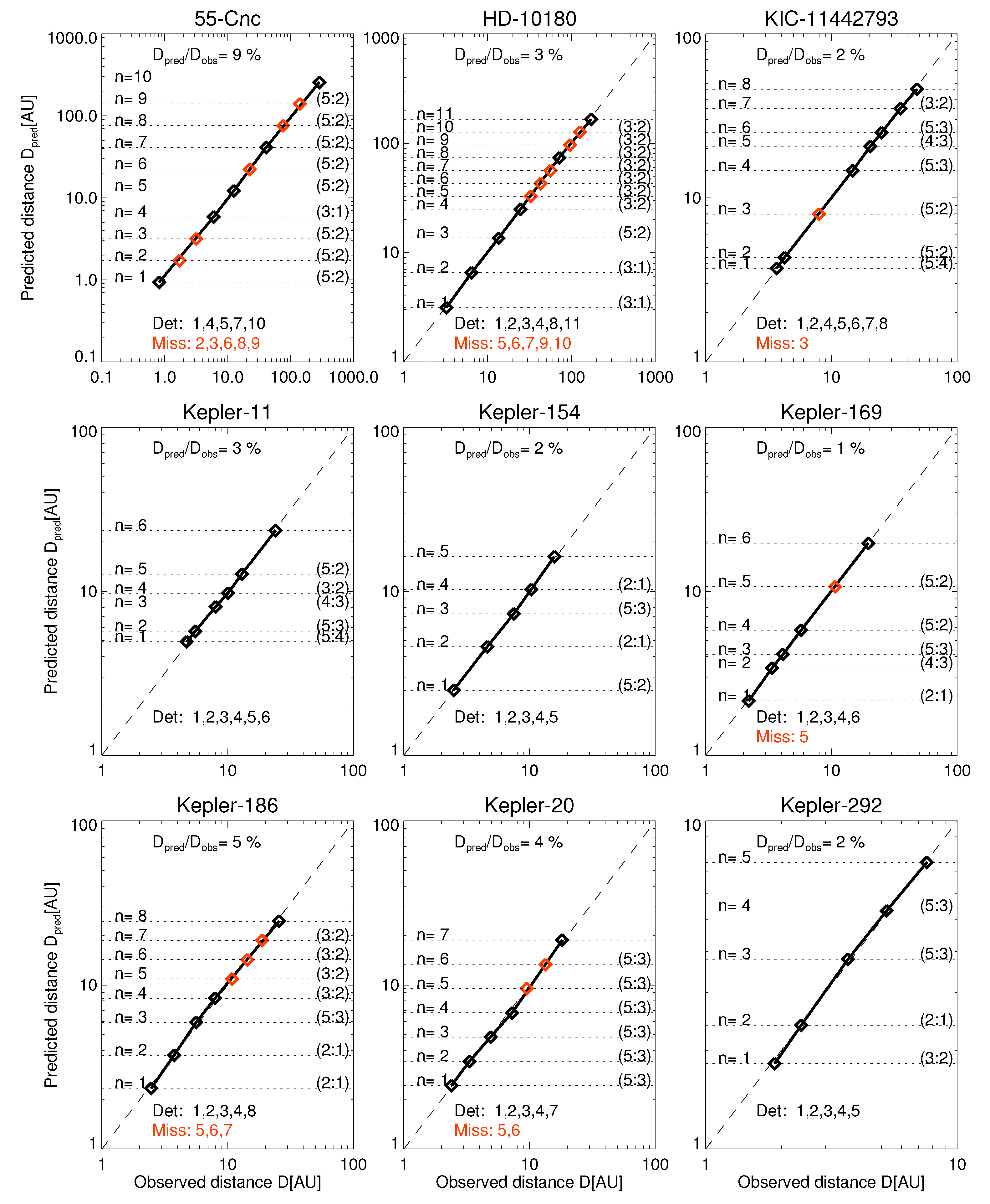
Figure 3.
Exoplanets, with representation similar to Figure 2.
Figure 3.
Exoplanets, with representation similar to Figure 2.

Figure 4.
Solar and planetary systems, with representation similar to Figure 2.
Figure 4.
Solar and planetary systems, with representation similar to Figure 2.

Table 1.
Statistics of analyzed data set, using the Exoplanet Orbit Database (EOD) at exoplanets.org (status as of 10 May 2017).
Table 1.
Statistics of analyzed data set, using the Exoplanet Orbit Database (EOD) at exoplanets.org (status as of 10 May 2017).
| Data Set | Number |
|---|---|
| Number of detected exoplanets | 5454 |
| Number of exoplanet-associated stars | 4522 |
| Number of stars with one exoplanet | 3860 |
| Number of stars with two exoplanets | 472 |
| Number of stars with three exoplanets | 128 |
| Number of stars with four exoplanets | 44 |
| Number of stars with five exoplanets | 14 |
| Number of stars with six exoplanets | 2 |
| Number of stars with seven exoplanets | 2 |
| Number of planet-pair orbit ratios | 932 |
Table 2.
Observed and predicted (in parentheses) distances of exoplanets.
| Star | Planet Distances (in Units of AU) |
|---|---|
| 55-Cnc | 0.82, (1.50), (2.77), 5.10, 10.60, (19.53), 35.98, (66.27), (122.07), 224.85 |
| 61-Vir | 2.61, (5.43), 11.29, 23.48 |
| GJ-163 | 4.21, 8.75, (12.30), (17.29), (24.31), (34.18), (48.04), 67.53 |
| GJ-581 | 2.15, 3.02, 5.56 |
| GJ-876 | 1.55, (2.86), (5.27), 9.71, 15.42, 24.48 |
| HD-10180 | 3.21, 6.68, 13.90, 25.61, (33.56), (43.97), (57.62), 75.50, (98.94), (129.64), 169.88 |
| HD-181433 | 4.45, (8.19), (15.09), (27.79), (51.18), 94.28, 173.67 |
| HD-20794 | 6.95, 11.03, 20.32 |
| HD-37124 | 28.78, (53.01), 97.64, 155.00 |
| HD-40307 | 2.65, 4.21, 6.68 |
| HD-69830 | 4.22, (5.53), (7.24), 9.49, (12.44), (16.30), (21.36), (27.99), 36.68 |
| HD-7924 | 3.08, 6.40, 9.00 |
| HIP-14810 | 3.54, (4.98), (7.00), (9.85), (13.84), (19.46), 27.35, (38.45), (54.05), (75.98), 106.80 |
| HIP-57274 | 4.04, (5.69), (7.99), 11.24, (15.79), (22.20), (31.21), (43.87), 61.67 |
| HR-8799 | 646.08, 1190.08, 1889.14, 2998.82 |
| K2-3 | 4.66, 8.58, 12.06 |
| KIC-11442793 | 3.66, 4.25, (7.83), 14.42, 20.27, 24.55, 34.52, 45.23 |
| KOI-1082 | 2.56, 3.60, 4.72 |
| KOI-1358 | 1.77, 2.31, 3.03, 3.97 |
| KOI-1475 | 1.37, 2.86, 4.53 |
| KOI-1563 | 2.17, 3.06, 4.00 |
| KOI-1576 | 4.77, 5.53, 7.78 |
| KOI-1590 | 1.77, 2.81, 5.18 |
| KOI-1681 | 1.58, 2.23, 3.53, (4.63), (6.07), 7.95 |
| KOI-1860 | 2.12, 3.36, 5.33, 8.46 |
| KOI-2037 | 3.11, 4.07, (8.47), 17.62 |
| KOI-2093 | 0.99, 1.83, 3.38 |
| KOI-2169 | 1.69, 2.21, 2.68 |
| KOI-2174 | 3.55, 4.12, (6.54), 10.39 |
| KOI-2248 | 1.91, 2.22, 4.62 |
| KOI-2433 | 3.33, (4.67), (6.57), 9.24, 14.66, 19.21 |
| KOI-2579 | 1.95, 2.37, 4.92 |
| KOI-279 | 3.84, 6.09, 9.67 |
| KOI-285 | 5.74, 9.11, 14.46 |
| KOI-2859 | 2.04, 2.67, 3.10 |
| KOI-3083 | 3.39, 4.10, 4.76 |
| KOI-3425 | 2.15, 3.96, 7.30 |
| KOI-3444 | 1.91, (3.03), 4.81, 5.58, (8.86), 14.06 |
| KOI-353 | 4.99, 9.20, (12.06), (15.80), (20.70), 27.13 |
| KOI-4524 | 2.23, 2.71, 3.80 |
| KOI-6242 | 18.07, 20.97, 38.63 |
| KOI-85 | 1.67, 3.07, 3.72 |
| KOI-94 | 2.41, 5.01, 7.96, 14.66 |
| KOI-945 | 8.74, 11.46, 16.10 |
| Kepler-102 | 3.03, 4.82, 6.31, 8.87 |
| Kepler-106 | 3.36, 5.34, (6.99), (9.16), 12.01 |
| Kepler-107 | 2.16, 2.83, 3.98, 6.32 |
| Kepler-11 | 4.74, 5.49, 7.72, 9.36, 12.26, 22.59 |
| Kepler-122 | 3.22, 5.10, 7.18, 10.09 |
| Kepler-124 | 2.27, (3.60), 5.71, 9.06 |
| Kepler-1254 | 2.35, 3.30, 4.64 |
| Kepler-126 | 4.79, 7.61, (10.70), (15.04), 21.14 |
| Kepler-127 | 5.93, 9.41, 13.23 |
| Kepler-132 | 3.37, 3.91, 8.13, (10.65), (13.95), (18.29), 23.96 |
| Kepler-1388 | 3.13, 4.97, 6.98, 9.82 |
| Kepler-142 | 1.60, 2.95, (6.13), 12.75 |
| Kepler-148 | 1.44, 2.65, (3.73), (5.24), (7.37), (10.36), 14.57 |
| Kepler-149 | 9.48, 15.05, 31.31 |
| Kepler-150 | 2.27, 3.61, 5.07, 9.34 |
| Kepler-154 | 2.49, 4.59, 7.29, 10.24, 16.26 |
| Kepler-1542 | 2.03, 2.46, 2.85, 3.31 |
| Kepler-157 | 1.44, (2.29), 3.63, 5.77 |
| Kepler-164 | 2.94, 4.66, 8.59 |
| Kepler-166 | 1.34, (1.89), (2.65), 3.73, (5.24), (7.36), 10.35 |
| Kepler-169 | 2.19, 3.48, 4.22, 5.93, (10.93), 20.13 |
| Kepler-171 | 2.59, 5.39, (7.06), (9.25), 12.12 |
| Kepler-172 | 2.05, 3.26, 6.00, 11.05 |
| Kepler-174 | 5.80, (7.61), (9.97), 13.06, (17.11), (22.42), (29.38), 38.50 |
| Kepler-176 | 3.09, 5.69, 9.04, 14.34 |
| Kepler-178 | 4.51, 7.16, (9.38), (12.29), (16.11), 21.11 |
| Kepler-18 | 2.31, 3.66, 5.81 |
| Kepler-184 | 4.85, 7.70, 10.09 |
| Kepler-186 | 2.47, 3.92, 6.23, 8.76, (11.47), (15.04), (19.70), 25.82 |
| Kepler-191 | 3.28, 4.61, 6.48 |
| Kepler-192 | 3.47, 4.55, 7.22 |
| Kepler-194 | 1.64, (2.60), (4.12), 6.54, 13.61 |
| Kepler-197 | 3.15, 5.01, 6.56, 9.22 |
| Kepler-198 | 1.20, (1.68), (2.37), (3.33), (4.68), 6.58, 13.68 |
| Kepler-20 | 2.39, 3.36, 4.72, 6.64, (9.33), (13.12), 18.45 |
| Kepler-203 | 2.15, 3.03, 4.81 |
| Kepler-206 | 3.93, 5.52, 7.76 |
| Kepler-207 | 1.37, 2.18, 3.46 |
| Kepler-208 | 2.61, 3.68, 4.82, 6.31 |
| Kepler-215 | 4.44, 5.82, 9.24, 14.67 |
| Kepler-217 | 2.47, 2.99, 4.21 |
| Kepler-218 | 2.36, (3.09), (4.05), (5.30), (6.95), (9.11), 11.93, 24.82 |
| Kepler-219 | 2.76, (3.62), (4.74), (6.21), 8.14, 12.92 |
| Kepler-220 | 2.59, 4.11, (5.38), (7.05), 9.24, 12.99 |
| Kepler-221 | 1.98, 3.15, 4.43, 6.23 |
| Kepler-222 | 2.49, 4.59, 9.55 |
| Kepler-223 | 3.79, 4.59, 6.02, 7.29 |
| Kepler-224 | 2.14, 3.40, 5.40, 7.58 |
| Kepler-226 | 2.50, 3.02, 3.96 |
| Kepler-228 | 1.87, 2.64, 4.85 |
| Kepler-229 | 3.39, 6.25, 11.52 |
| Kepler-23 | 3.70, 4.84, 6.35 |
| Kepler-235 | 2.23, 4.12, 7.58, 13.97 |
| Kepler-238 | 1.64, 3.40, 5.40 |
| Kepler-24 | 2.62, 5.45, 7.15 |
| Kepler-244 | 2.65, 4.88, 7.75 |
| Kepler-245 | 2.18, 4.02, 7.40, 11.74 |
| Kepler-247 | 2.23, 4.64, 7.37 |
| Kepler-249 | 2.22, 3.52, 5.59 |
| Kepler-250 | 2.58, 3.63, 6.68 |
| Kepler-251 | 2.84, (3.72), (4.88), 6.39, 8.99, (11.78), (15.43), 20.22 |
| Kepler-253 | 2.43, 4.47, 6.29 |
| Kepler-254 | 3.24, 5.14, 6.74 |
| Kepler-255 | 1.03, (1.35), (1.77), (2.32), 3.04, 4.27 |
| Kepler-256 | 1.38, 2.19, 3.08, 4.33 |
| Kepler-257 | 1.78, 3.71, (4.86), (6.37), 8.35 |
| Kepler-26 | 2.32, (3.69), 5.86, 7.10, 13.07 |
| Kepler-265 | 3.61, 6.64, 12.23, 16.03 |
| Kepler-267 | 2.24, 3.56, (5.65), 8.96 |
| Kepler-271 | 3.01, 3.49, 4.23 |
| Kepler-272 | 2.07, 3.28, 4.61 |
| Kepler-275 | 4.73, 6.20, 9.85 |
| Kepler-286 | 1.48, 2.35, 3.30, (4.32), (5.66), (7.42), 9.72 |
| Kepler-288 | 3.34, 6.94, 14.44 |
| Kepler-289 | 10.61, 16.84, 26.73 |
| Kepler-292 | 1.88, 2.47, 3.91, 5.50, 7.73 |
| Kepler-295 | 5.43, 7.63, 10.00 |
| Kepler-296 | 2.36, 3.32, (4.34), (5.69), 7.46, 10.49, 16.64 |
| Kepler-298 | 4.79, 7.60, (9.96), (13.05), 17.10 |
| Kepler-299 | 2.05, 3.77, 5.98, 11.02 |
| Kepler-30 | 9.51, 15.10, 27.81 |
| Kepler-301 | 1.85, 2.93, 5.40 |
| Kepler-304 | 1.31, 2.08, 2.92, 4.11 |
| Kepler-306 | 2.78, 3.65, 6.72, 12.38 |
| Kepler-31 | 7.58, 12.03, 19.10 |
| Kepler-310 | 5.79, (9.19), 14.59, 20.51 |
| Kepler-319 | 2.67, 3.75, (5.28), (7.42), 10.43 |
| Kepler-32 | 0.82, (1.30), 2.07, 3.28, 4.30, 7.92 |
| Kepler-325 | 2.74, 5.71, 11.87 |
| Kepler-326 | 1.72, 2.72, 3.57 |
| Kepler-327 | 1.87, 2.96, 5.46 |
| Kepler-33 | 3.18, 5.86, 8.23, 10.79, 12.52 |
| Kepler-331 | 4.15, 6.59, 10.46 |
| Kepler-332 | 3.87, 6.15, 9.76 |
| Kepler-334 | 3.10, 5.72, 9.08 |
| Kepler-336 | 1.60, (2.10), (2.75), (3.60), 4.72, 7.49 |
| Kepler-338 | 5.73, 8.06, 11.33 |
| Kepler-339 | 2.92, 3.53, 4.63 |
| Kepler-341 | 3.00, 3.93, (5.15), (6.75), 8.84, 11.59 |
| Kepler-342 | 1.39, (2.90), 6.03, 8.47, 11.10 |
| Kepler-351 | 11.11, 14.56, 26.83 |
| Kepler-354 | 3.11, 6.46, 8.47 |
| Kepler-357 | 3.47, 6.40, 13.31 |
| Kepler-359 | 8.68, 15.98, 19.36 |
| Kepler-363 | 2.36, 3.74, 4.90 |
| Kepler-37 | 5.63, 7.92, 12.57 |
| Kepler-372 | 3.61, 7.50, 9.83 |
| Kepler-374 | 1.53, 2.15, 2.82 |
| Kepler-398 | 2.55, 3.59, 5.05 |
| Kepler-399 | 5.93, 9.41, 14.93 |
| Kepler-401 | 5.91, (7.75), (10.16), 13.31, (17.44), (22.85), 29.94 |
| Kepler-402 | 2.53, 3.32, 4.35, 5.04 |
| Kepler-403 | 3.67, 5.83, (9.25), 14.68 |
| Kepler-42 | 0.59, 1.09, 1.42 |
| Kepler-431 | 3.59, 4.17, 5.05 |
| Kepler-444 | 2.35, 2.73, 3.30, 3.83, 4.45 |
| Kepler-445 | 2.07, 2.91, 4.10 |
| Kepler-446 | 1.35, 2.14, 3.01 |
| Kepler-48 | 2.84, 4.50, (6.33), (8.90), 12.51 |
| Kepler-49 | 1.88, 3.91, 5.12, 7.20 |
| Kepler-52 | 3.96, 6.28, 9.98 |
| Kepler-53 | 4.56, 7.25, 11.50 |
| Kepler-54 | 4.00, 5.25, 7.37 |
| Kepler-55 | 1.70, 2.69, 4.28, 7.88, 10.32 |
| Kepler-58 | 4.71, 6.17, 11.37 |
| Kepler-60 | 3.71, 4.30, 5.21 |
| Kepler-603 | 3.38, (4.43), (5.81), 7.61, (9.97), (13.06), (17.12), 22.43 |
| Kepler-62 | 3.20, 5.07, 6.65, (8.71), (11.42), (14.96), (19.60), 25.69, 40.78 |
| Kepler-68 | 3.08, 4.33, (6.87), (10.90), (17.30), (27.47), (43.60), 69.22 |
| Kepler-758 | 2.83, 3.98, 5.21, 7.32 |
| Kepler-770 | 1.30, 2.70, (3.79), (5.33), 7.49 |
| Kepler-79 | 5.67, 8.99, 14.28, 18.71 |
| Kepler-80 | 0.99, 2.06, 2.70, 3.54, 4.29 |
| Kepler-81 | 3.29, 5.22, 7.33 |
| Kepler-82 | 1.78, 3.29, (4.62), (6.49), 9.13, 14.49 |
| Kepler-83 | 2.99, 4.75, 7.53 |
| Kepler-84 | 2.61, 4.15, 5.44, 8.63, 12.13 |
| Kepler-85 | 4.10, 5.37, 7.04, 8.53 |
| Kepler-89 | 2.41, 5.01, 7.96, 14.66 |
| Kepler-9 | 1.36, (1.92), (2.70), (3.79), (5.33), 7.49, 11.88 |
| PSR-B1257+12 | 8.61, 15.86, 20.78 |
| TRAPPIST-1 | 1.32, 1.85, 2.60, 3.41, 4.47, 5.41, 7.09 |
| WASP-47 | 2.59, 4.11, (6.52), (10.34), (16.42), (26.07), (41.38), 65.69 |
| mu-Ara | 4.53, (8.34), (15.37), (28.31), 52.14, 82.77, (152.46), 280.84 |
| upsilon-And | 2.77, (5.11), (9.41), (17.33), 31.92, (58.80), 108.31 |
© 2017 by the authors. Licensee MDPI, Basel, Switzerland. This article is an open access article distributed under the terms and conditions of the Creative Commons Attribution (CC BY) license (http://creativecommons.org/licenses/by/4.0/).
Share and Cite
MDPI and ACS Style
Aschwanden, M.J.; Scholkmann, F. Exoplanet Predictions Based on Harmonic Orbit Resonances. Galaxies 2017, 5, 56. https://doi.org/10.3390/galaxies5040056
AMA Style
Aschwanden MJ, Scholkmann F. Exoplanet Predictions Based on Harmonic Orbit Resonances. Galaxies. 2017; 5(4):56. https://doi.org/10.3390/galaxies5040056
Chicago/Turabian StyleAschwanden, Markus J., and Felix Scholkmann. 2017. "Exoplanet Predictions Based on Harmonic Orbit Resonances" Galaxies 5, no. 4: 56. https://doi.org/10.3390/galaxies5040056
Note that from the first issue of 2016, this journal uses article numbers instead of page numbers. See further details here.