Synchrotron Radiation Maps from Relativistic MHD Jet Simulations


1
Centre for mathematical Plasma Astrophysics, Department of Mathematics, KU Leuven, 3001 Leuven, Belgium
2
Institut für Theoretische Physik, Goethe Universiteit Frankfurt, 60438 Frankfurt am Main, Germany
*
Author to whom correspondence should be addressed.
Galaxies 2017, 5(4), 79; https://doi.org/10.3390/galaxies5040079
Submission received: 15 September 2017
/
Revised: 8 November 2017
/
Accepted: 10 November 2017
/
Published: 15 November 2017
(This article belongs to the Special Issue Polarised Emission from Astrophysical Jets)
Abstract
:Relativistic jets from active galactic nuclei (AGN) often display a non-uniform structure and are, under certain conditions, susceptible to a number of instabilities. An interesting example is the development of non-axisymmetric, Rayleigh-Taylor type instabilities in the case of differentially rotating two-component jets, with the toroidal component of the magnetic field playing a key role in the development or suppression of these instabilities. We have shown that higher magnetization leads to stability against these non-axisymmetric instabilities. Using ray-casting on data from relativistic MHD simulations of two-component jets, we now investigate the effect of these instabilities on the synchrotron emission pattern from the jets. We recover many well known trends from actual observations, e.g., regarding the polarization fraction and the distribution of the position angle of the electric field, in addition to a different emitting region, depending on the stability of the jet.
1. Introduction
Astrophysical jets, originating from sources ranging from young stars (YSO jets) to active galaxies (AGN jets), have been observed in various wavelengths and in some cases a complex structure has been revealed. The evolution, acceleration and collimation of jets is often associated with the presence of a magnetic field and specifically, with the conversion of magnetic to kinetic energy and the effect of the hoop stress.
On many occasions, astrophysical jets display a two-component structure, i.e., a non-uniform profile perpendicular to the jet axis. Evidence for this structure can be found, e.g., in the case of blazars in [1]. A usual description for these jets includes a fast spine and a slower sheath configuration, which may in turn affect the stability of these outflows. An example is the development of Rayleigh-Taylor type instabilities, induced by differential rotation [2,3,4,5].
Observations, polarimetric and rotation measure (RM) studies, e.g., from Very Long Baseline Interferometry (VLBI), have been extensively carried out in the last decades and can be used to determine the morphology of these outflows. In particular, spine and sheath structures may also be observed in terms of polarization and RM, which can in turn provide information on the topology of the magnetic field [6]. Such observations often give evidence for the existence of a large scale, helical magnetic field [7]. Furthermore, analysis of the distribution of the position angle of the electric field vector (EVPA) concludes that in general, EVPAs are roughly perpendicular or parallel to the direction of the flow, with “jumps” being also observed in some objects [8].
In this work, we intend to examine any possible effects of this (in)stability on the emission pattern observed from a two-component jet. For this, we will use existing results from relativistic, magnetohydrodynamic (MHD) simulations of two-component jets, presented in [4]. We will assume an optically thin emission from the inner jet only and, as a first approximation, ignore absorption and Faraday rotation from the outer jet. This is implied by actual observations of specific objects (e.g., [9]) and from the fact that for small viewing angles, the higher Lorentz factor (and by extension the higher Doppler boost) lead to a stronger emission from the inner jet.
2. Materials and Methods
For the relativistic two-component jet simulations, we used the parallel, grid adaptive MPI-AMRVAC code (MPI-Adaptive Mesh Refinement-Versatile Advection Code) [10], under the assumption of a translational symmetry along the z axis. We will adopt the same recipe for the configuration of the jet and the normalization as described in [3]. Velocity is normalized in units of c, distance is measured in and mass is normalized to proton mass .
First we fix the (outer) radius of the jet at = 0.1 and the inner radius is arbitrarily chosen to be . These values are consistent with [11] and recently [12], where the half opening angle of the M87 jet was found ~2 at a distance of ~4 and the jet is almost fully collimated at the same scale. The next step is to define the initial conditions for the density, velocity, magnetic field and pressure profiles of the jet (inner and outer regions) and the surrounding, external (static and unmagnetized) medium.
We fix an initial toroidal velocity profile:
where for the inner jet, for the outer jet and (which leads to continuity of at the interface). Thus increases with R until , then decreases, with a maximum value at .
For the poloidal velocity, we assume a constant value in each component, so that the corresponding Lorentz factor is for the inner jet and for the outer jet, in agreement with [13]. We note that this is the dominant component of the velocity and the total Lorentz factor can be approximated as and respectively.
The magnetic field is described in a similar way: a constant poloidal component in each part of the jet () while the toroidal component resembles the form of the toroidal velocity:
The constants are defined by the maximum magnetization of the jet, at . We use values of ranging from to , so the jet is kinetically dominated. Similar to the definition of the toroidal velocity, we select , while the poloidal magnetic field will still be discontinuous at .
Regarding the density, we assume a constant value in each part of the jet and the external medium:
The kinetic luminosity flux and the percentage carried by the inner part are used to calculate the density ratio of the above regions. Assuming a kinetic luminosity flux of ~10 ergs/s, of which 1% is carried by the inner jet, we find that and . A visualization of the initial conditions (density, toroidal velocity) can be found in [4].
The polarized state of the emitted radiation is often described via the Stokes parameters , with I corresponding to its intensity. In the most general case of elliptically polarized light, are non-zero, with the first two quantifying the ellipse and V quantifies the circular polarization. The linear fractional polarization can be calculated from the Stokes parameters, using the formula:
The EVPA in the observer’s frame can be calculated from the formulas:
For the ray-casting, we assume an optically thin synchrotron emission regime, where the emitting region is masked via the value of the Lorentz factor and the density, suitably chosen to correspond to the inner jet. The values used for masking the emitting region are obtained from analysis of the final state of the jet, so that the outer jet is ignored at all stages of the ray-casting procedure. The emission is connected to the frequency via a power law ~, where is the emission coefficient.
We will restrict our study to linear polarization only, as circular polarization is in most cases but a small fraction of the observed polarized emission.
Since we now ignore absorption, the unpolarized transfer equation reduces to:
In this case, only the total intensity is treated whereas for the linearly polarized case, Stokes are also taken into account.
The calculations are made in the co-moving frame, where the magnetic field is [14]:
3. Results
In the following subsections, we present the results from the MHD jet simulations and the ray-casting.
3.1. Simulations
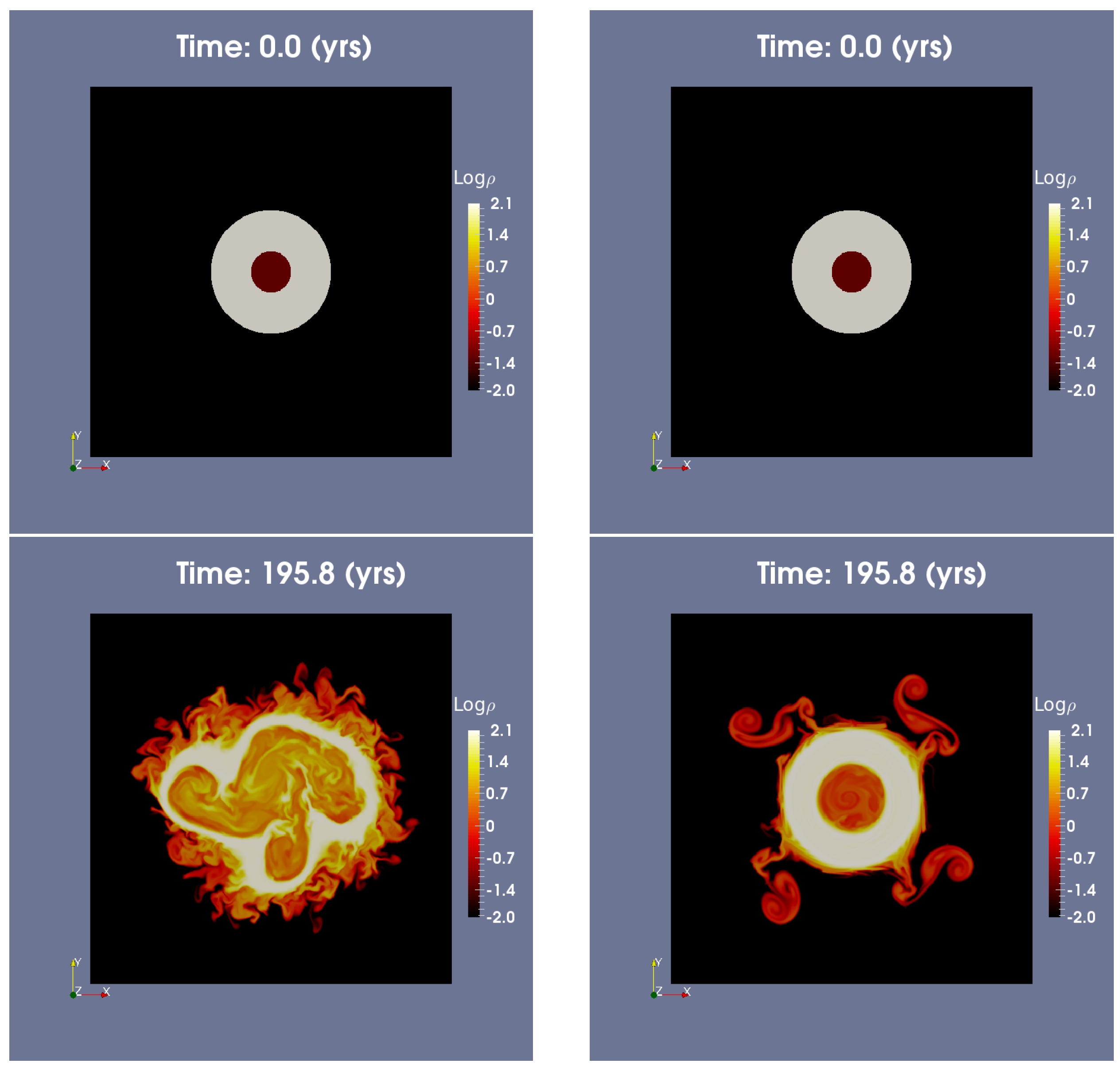
As mentioned in the previous section, we present results from our 2.5D simulations for two different values of magnetization, and , which respond to Case I and Case III from [4]. We follow the evolution up to 3 rotations of the inner jet, where equals approximately 196 years. We first determine the stability or instability of the jet via the density distribution and the average Lorentz factor of the inner jet.
In the first case, where the magnetic field has a weak toroidal component, there is strong mixing between the two parts of the outflow and a considerable expansion of the jet cross section. On the other hand, the second case results in a still collimated jet (Figure 1). We also note a considerable deceleration of the inner jet, quantified via the decrease of the average Lorentz factor of the inner jet (~11 after 3 rotations of the inner jet). In the second case, we end up with a more stable outflow, the mixing between the two components is greatly reduced and the deceleration of the inner jet occurs at a lower rate (~22 after 3 rotations of the inner jet).
3.2. Ray-casting
We use the results from the simulations presented in Section 3.1 to examine the effect of these instabilities in the emitting pattern. Taking into account an optically thin emission from the inner jet only, we will examine the intensity (Stokes I), the polarized intensity and the EVPA for each case. We assume a frequency of GHz for the emitted radiation and a spectral index of .
Post-processing the simulation data enables masking the emitting region based on the density and the Lorentz factor of the outflow. The masking value for the Lorentz factor is set to for both simulations, whereas the values for the density are and for and respectively. These are representative values of the inner jet for each case, as found in the final state of the simulations.
The total intensity maps (Stokes I) presented in Figure 2 for the above mentioned cases, assume a viewing angle of between the jet axis and the line of sight. Intensity values are normalized with respect to the highest value, which makes it easier to identify regions where the emission is stronger. The bulk of the emission follows the inner jet, with the maximum values located in specific regions near the interface of the two components. These bright spots coincide with regions where the magnitude of the magnetic field is maximum, as obtained from the MHD simulations at .
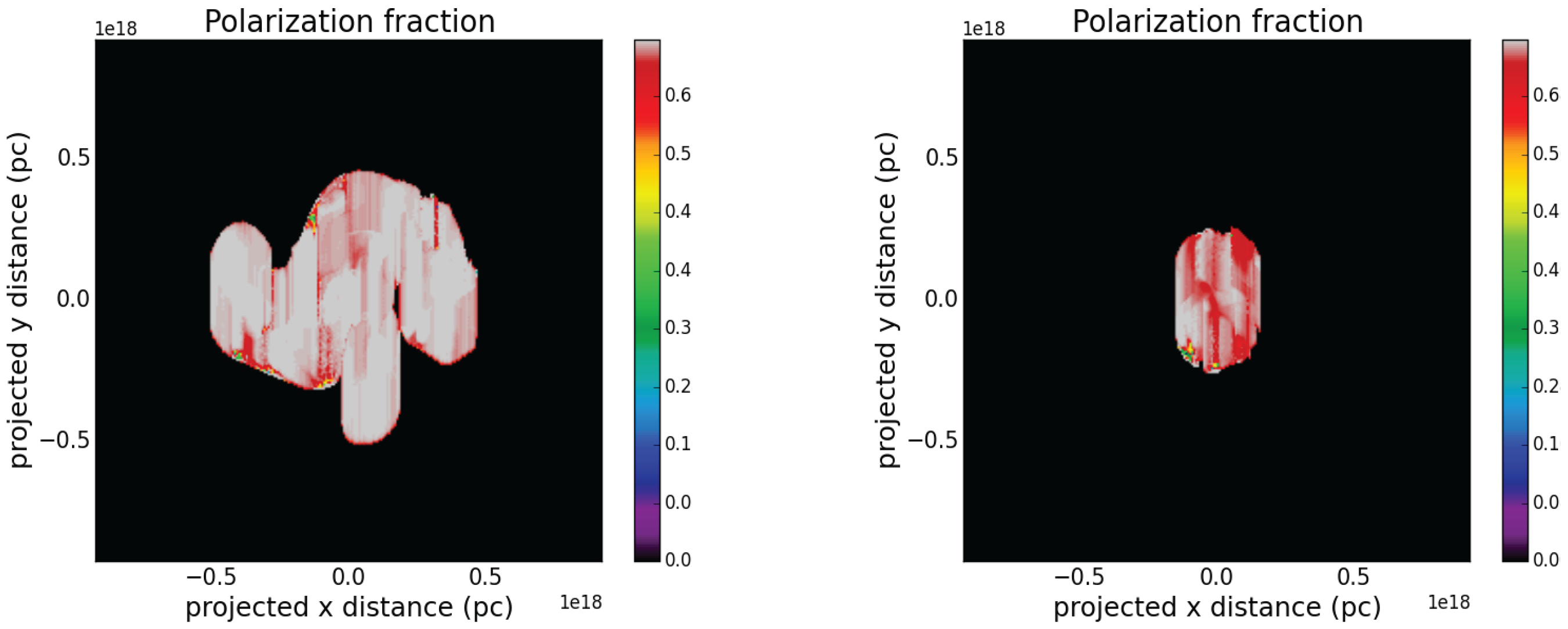
The polarized intensity maps (Figure 3) obtained from these simulations follow the same pattern:
As expected, the polarized intensity maps resemble the intensity maps. A more interesting result is however to determine the maximum degree of polarization and its distribution, which is presented in Figure 4. In both cases, the maximum value is ~70%, which is the theoretical limit for a uniformly oriented magnetic field, for p~2–3.
4. Discussion
We find that the transverse stability (i.e., normal to the jet axis) of a two-component jet is associated with the magnetization of the outflow and by extension with the magnitude of the toroidal magnetic field component. Outflows with lower values of magnetization result in an unstable configuration, decollimation and finally a decelerating jet, while higher values lead to stability. For a more detailed presentation, see [4].
Post-processing the simulation data and using ray-casting reveals that these instabilities, as expected, have an effect on the emission. We examined linear polarization only, as observations show that circular polarization is only but a small fraction.
In the unstable case (with ), the emitting region is extended (as the inner jet also expands), with higher emission being detected in specific parts of the mixed region where the magnetic field is stronger. The stable case (with ) on the other hand, displays a more ordered, smaller emitting region, where again highest emission is located near the interface between the inner and the outer jet, due to the higher magnetic field magnitude.
Overall, we retrieve well known observed trends of AGN jets. This can be seen initially in terms of e.g., the distribution of EVPA. EVPAs, as seen in Figure 2 and Figure 3, are in general perpendicular to the jet axis or aligned to the flow (for larger viewing angles not shown here). In the case with , we also notice a divergence in the direction of EVPAs. Finally, the maximum polarization fraction is ~70% for both cases.
Future work will focus on a more physically realistic approach in our ray-casting procedure, including absorption and Faraday rotation, for different frequencies and viewing angles. We also note that the almost uniform, close to the theoretical maximum value of the polarization fraction, might be due to integrating at a small viewing angle and requires further investigation, including a parametric study of different . The same methods will also be applied to already existing 3D simulation data.
Acknowledgments
This research was supported by projects GOA/2015-014 (2014–2018 KU Leuven) and the Interuniversity Attraction Poles Programme by the Belgian Science Policy Office (IAP P7/08 CHARM). The computational resources and services used in this work were provided by the VSC (Flemish Supercomputer Center), funded by the Research Foundation Flanders (FWO) and the Flemish Government—department EWI. Visualization was performed using Paraview (more information on www.paraview.org) and Python (https://www.python.org/).
Author Contributions
D.M. and R.K. conceived the simulations; D.M. performed the simulations, the ray-casting and analyzed the data; R.K. and O.P. developed the MHD code; O.P. designed the ray-casting code and provided technical support; D.M. wrote the paper.
Conflicts of Interest
The authors declare no conflict of interest.
References
- Ghisellini, G.; Tavecchio, F.; Chiaberge, M. Structured jets in TeV BL Lac objects and radiogalaxies. Implications for the observed properties. Astron. Astrophys. 2005, 432, 401–410. [Google Scholar] [CrossRef]
- Meliani, Z.; Keppens, R. Transverse stability of relativistic two-component jets. Astron. Astrophys. 2007, 475, 785–789. [Google Scholar] [CrossRef]
- Meliani, Z.; Keppens, R. Decelerating Relativistic Two-Component Jets. Astrophys. J. 2009, 705, 1594–1606. [Google Scholar] [CrossRef]
- Millas, D.; Keppens, R.; Meliani, Z. Rotation and magnetic field effects on the stability of two-component jets. Mon. Not. R. Astron. Soc. 2017, 470, 592–605. [Google Scholar] [CrossRef]
- Toma, K.; Komissarov, S.S.; Porth, O. Rayleigh-Taylor Instability in Two-Component Relativistic Jets. arXiv, 2017; arXiv:1705.10425v2. [Google Scholar]
- Gabuzda, D.; Reichstein, A.; O’Neill, E.L. Are spine-sheath polarization structures in the jets of active galactic nuclei associated with helical magnetic fields? Mon. Not. R. Astron. Soc. 2014, 444, 172–184. [Google Scholar] [CrossRef]
- Gabuzda, D.C.; Knuettel, S.; Reardon, B. Transverse Faraday-rotation gradients across the jets of 15 active galactic nuclei. Mon. Not. R. Astron. Soc. 2015, 450, 2441–2450. [Google Scholar] [CrossRef]
- Pushkarev, A.B.; Gabuzda, D.C.; Vetukhnovskaya, Y.N.; Yakimov, V.E. Spine-sheath polarization structures in four active galactic nuclei jets. Mon. Not. R. Astron. Soc. 2005, 356, 859–871. [Google Scholar] [CrossRef]
- Tavecchio, F.; Ghisellini, G. On the magnetization of BL Lac jets. Mon. Not. R. Astron. Soc. 2016, 456, 2374–2382. [Google Scholar] [CrossRef]
- Porth, O.; Xia, C.; Hendrix, T.; Moschou, S.P.; Keppens, R. MPI-AMRVAC for Solar and Astrophysics. Astrophys. J. Suppl. Ser. 2014, 214, 4–29. [Google Scholar] [CrossRef]
- Biretta, J.A.; Junor, W.; Livio, M. Evidence for initial jet formation by an accretion disk in the radio galaxy M87. New Astron. Rev. 2002, 46, 239–245. [Google Scholar] [CrossRef]
- Asada, K.; Nakamura, M. The Structure of the M87 Jet: A Transition from Parabolic to Conical Streamline. Astrophys. J. 2012, 745, L28. [Google Scholar] [CrossRef]
- Giroletti, M.; Giovannini, G.; Feretti, L.; Cotton, W.D.; Edwards, P.G.; Lara, L.; Marscher, A.P.; Mattox, J.R.; Piner, B.G.; Venturi, T. Parsec-Scale Properties of Markarian 501. Astrophys. J. 2004, 600, 127–140. [Google Scholar] [CrossRef]
- Goedbloed, J.P.; Keppens, R.; Poedts, S. Ideal MHD in special relativity. In Advanced Magnetohydrodynamics; Cambridge University Press: Cambridge, UK, 2010; p. 565. ISBN 978-0-521-70524-0. [Google Scholar]
Figure 1.
Left: Density map at (top) and (bottom) for . Right: Density map at (top) and (bottom) for . The shown plane is perpendicular to the jet axis.
Figure 1.
Left: Density map at (top) and (bottom) for . Right: Density map at (top) and (bottom) for . The shown plane is perpendicular to the jet axis.

Figure 2.
Left: Normalized intensity map (Stokes I) at (top) and (bottom) for . Right: Normalized intensity map at (top) and (bottom) for . The arrows represent the electric field vector, as calculated from Equation (5). Viewing angle is , flow direction is outwards.
Figure 2.
Left: Normalized intensity map (Stokes I) at (top) and (bottom) for . Right: Normalized intensity map at (top) and (bottom) for . The arrows represent the electric field vector, as calculated from Equation (5). Viewing angle is , flow direction is outwards.
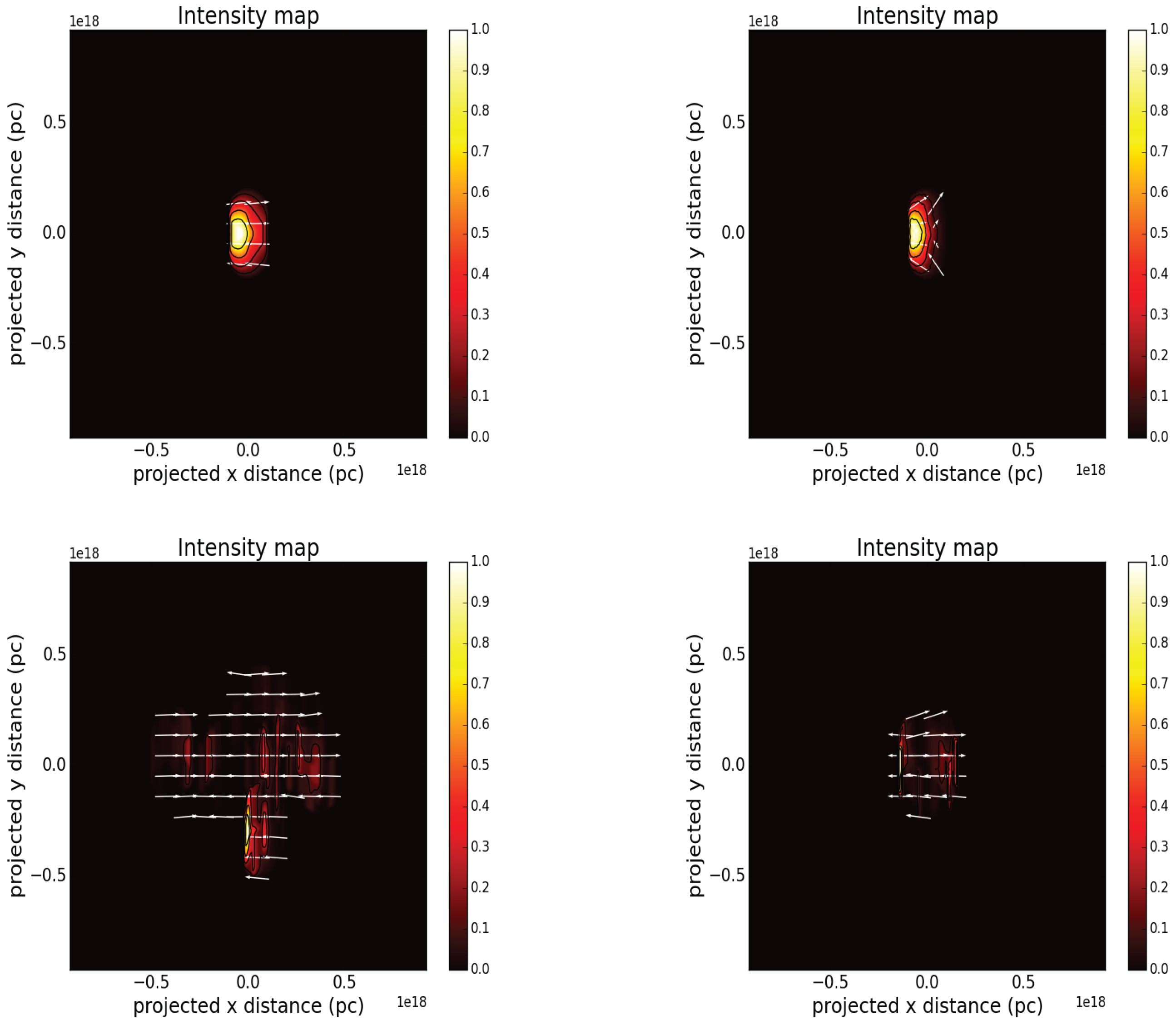
Figure 3.
Left: Polarized intensity (normalized) map at (top) and (bottom) for . Right: Polarized intensity (normalized) map at (top) and (bottom) for . The arrows represent the electric field vector, as calculated from Equation (5). Viewing angle is , flow direction is outwards.
Figure 3.
Left: Polarized intensity (normalized) map at (top) and (bottom) for . Right: Polarized intensity (normalized) map at (top) and (bottom) for . The arrows represent the electric field vector, as calculated from Equation (5). Viewing angle is , flow direction is outwards.
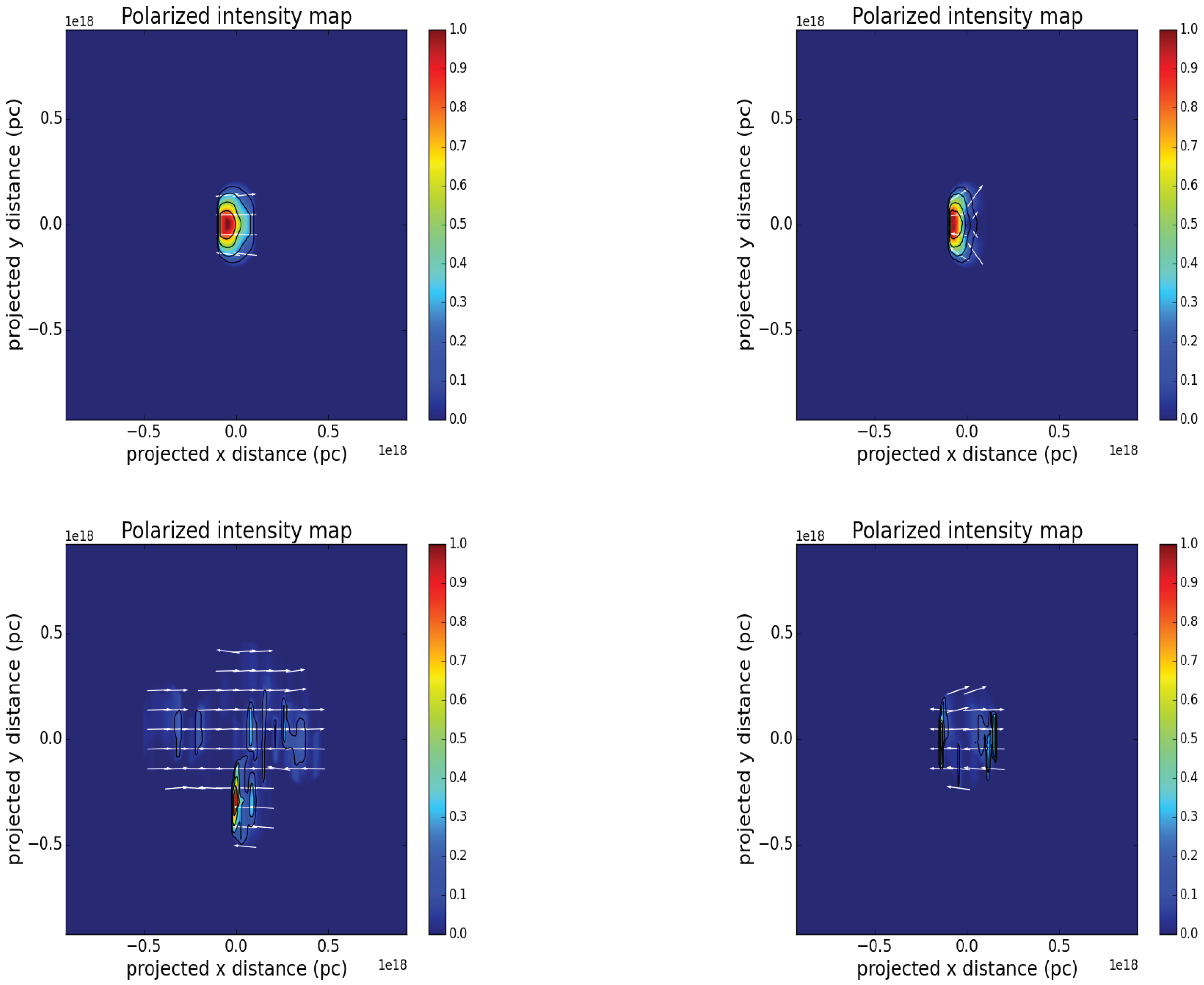
Figure 4.
Linear fractional polarization for cases with (left) and (right), at .

© 2017 by the authors. Licensee MDPI, Basel, Switzerland. This article is an open access article distributed under the terms and conditions of the Creative Commons Attribution (CC BY) license (http://creativecommons.org/licenses/by/4.0/).
Share and Cite
MDPI and ACS Style
Millas, D.; Porth, O.; Keppens, R. Synchrotron Radiation Maps from Relativistic MHD Jet Simulations. Galaxies 2017, 5, 79. https://doi.org/10.3390/galaxies5040079
AMA Style
Millas D, Porth O, Keppens R. Synchrotron Radiation Maps from Relativistic MHD Jet Simulations. Galaxies. 2017; 5(4):79. https://doi.org/10.3390/galaxies5040079
Chicago/Turabian StyleMillas, Dimitrios, Oliver Porth, and Rony Keppens. 2017. "Synchrotron Radiation Maps from Relativistic MHD Jet Simulations" Galaxies 5, no. 4: 79. https://doi.org/10.3390/galaxies5040079
Note that from the first issue of 2016, this journal uses article numbers instead of page numbers. See further details here.