Bell Inequality and Its Application to Cosmology

Abstract

One of the cornerstones of inflationary cosmology is that primordial density fluctuations have a quantum mechanical origin. However, most physicists consider that such quantum mechanical effects disappear in CMB data due to decoherence. In this conference report, we show that the violation of Bell inequalities in an initial state of our universe increases exponentially with the number of modes to measure in inflation. This indicates that some evidence that our universe has a quantum mechanical origin may survive in CMB data, even if quantum entanglement decays exponentially afterward due to decoherence.

1. Introduction

Quantum entanglement has fascinated many physicists because of its counterintuitive nature that one particle of an entangled pair instantaneously knows what measurement has been performed on the other, irrespective of their separation—even beyond the lightcone [1]. After Aspect et al. succeeded in showing experimental evidence of the quantum nature of entanglement by measuring correlations of linear polarizations of pairs of photons [2,3], much attention has been paid to this genuine quantum property in various research areas in quantum information theory.

Quantum entanglement should play an important role in cosmology. One of the cornerstones of inflationary cosmology is that primordial density fluctuations have a quantum mechanical origin. Hence, the initial state of the universe produced by inflation is highly entangled. It is desired to find compelling evidence for their quantum nature. Recently, Maldacena considered an inflationary scenario where one can prove the quantum origin of density fluctuations by performing the Bell inequality violating experiment during inflation [4].

In inflationary cosmology, the Bunch–Davies vacuum which is a two-mode squeezed state is usually assumed as the simplest initial state of quantum fluctuations of the universe. This is because spacetime looks flat at short distances, and then quantum fluctuations are expected to start in a minimum energy state. However, the latest Planck data show the possibility of deviation from the Bunch–Davies vacuum [5]. Motivated by this, there have been several attempts to find some observational signatures on the CMB when the initial state is a non-Bunch–Davies vacuum due to entanglement between two scalar fields [6,7] and between two universes [8]. If we apply the Bell inequalities violating experiment to cosmology, we may be able to prove the quantum origin of density fluctuations and find the nature of the initial state of the universe.

In this conference report based on our paper [9], we evaluate the Bell inequalities for the Bunch–Davies vacuum and a non-Bunch–Davies vacuum in inflation. We find that both vacua violate the Bell inequalities. Remarkably, as for the non-Bunch–Davies vacuum, the violation increases exponentially with the number of modes to measure. This implies that the Bell inequalities are useful to classify the initial quantum state of the universe.

The paper is organized as follows. In Section 2, we review Bell and Mermin–Klyshko inequalities. In Section 3, as cosmological initial states, we explain the Bunch–Davies vacuum expressed by a two-mode squeezed state and the non-Bunch–Davies vacuum expressed by a four-mode squeezed state. In Section 4, we present the result of the Bell inequalities for those cosmological initial states. Finally we summarize our result in Section 5.

2. Bell Inequalities

In this section, we review the Bell inequality with the simplest example of a pair of spins (a two-partite system) and Mermin–Klyshko inequalities for a multipartite system [10,11]. We call them Bell inequalities here and below. The Bell inequalities are violated by quantum entanglement and provide a criterion for discriminating the quantum entanglement from any local classical hidden variable theories [12,13]. The upper bound of the violation increases with the number of partite states [14,15].

2.1. Bell Inequality

We consider two sets of non-commuting operators A, $A^{\prime }$ and B, $B^{\prime }$. Those operators correspond to measuring the spin along various axes, and have eigenvalues $\pm 1$. They are expressed by the Pauli matrices ${\sigma }^i$ and unit vectors $n^i$ such as $A=n^i{\sigma }^i$. The Bell operator $\mathcal{B}$ is defined as

$$\begin{array}{c}\hfill \mathcal{B}=\frac{1}{2}\left(A\otimes B+A^{\prime }\otimes B+A\otimes B^{\prime }-A^{\prime }\otimes B^{\prime }\right),\end{array}$$

(1)

where the variables A, $A^{\prime }$ and B, $B^{\prime }$ are represented by Hermitian operators which act on the Hilbert spaces ${\mathcal{H}}_A$ and ${\mathcal{H}}_B$, respectively. If we rewrite it as a factorized form

$$\begin{array}{c}\hfill \mathcal{B}=\frac{1}{2}A\otimes \left(B+B^{\prime }\right)+\frac{1}{2}{A}^{\prime }\otimes \left(B-B^{\prime }\right),\end{array}$$

(2)

then we see that the first (second) term becomes $\pm 1$ while the second (first) one vanishes because we can have either $B=B^{\prime }$ or $B=-B^{\prime }$. In local classical hidden variable theories, the expectation value of $\mathcal{B}$ then gives $|\langle \mathcal{B}\rangle |\le 1$. In quantum mechanics, however, this Bell inequality can be violated for the expectation value of the quantum operator. It is easy to check that its square becomes1

$$\begin{array}{c}\hfill {\mathcal{B}}^2=I-\frac{1}{4}\left[A,A^{\prime }\right]\left[B,B^{\prime }\right],\end{array}$$

(3)

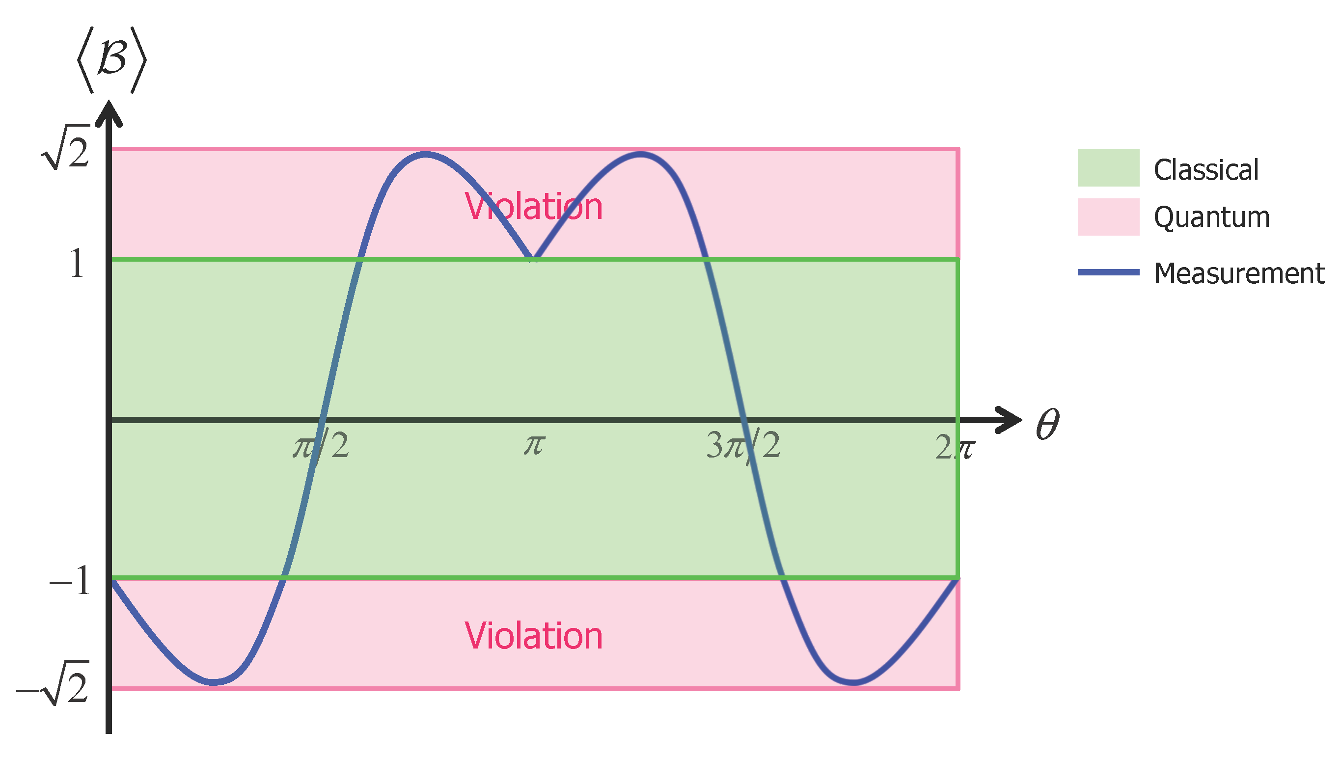
where we used the fact that the square of each operator is one, $A^2=I$, $A^{\prime 2}=I$, etc., and I is the identity operator. Since the commutators of the Pauli matrices are non-zero and each gives $2i$, we find that $\langle {\mathcal{B}}^2\rangle \le 2$ or $\left|\langle \mathcal{B}\rangle \right|\le \sqrt{2}$. Thus, the maximal violation of Bell inequality in quantum mechanics has the extra $\sqrt{2}$ factor in the case of a pair of spins [16]. This violation was convincingly tested by Aspect et al. [2,3] (see Figure 1) and the quantum entanglement was confirmed as a fundamental aspect of quantum mechanics.

2.2. Mermin–Klyshko Inequalities

The Bell inequality is generalized for a multipartite system, which is called Mermin–Klyshko inequalities. We write the operators $\{A,B,C,\cdots \}$ by $\{{\mathcal{O}}_1,{\mathcal{O}}_2,{\mathcal{O}}_3,\cdots \}$ below for later convenience. Defining ${\mathcal{B}}_1={\mathcal{O}}_1$ and ${\mathcal{B}}_1^{\prime }={\mathcal{O}}_1^{\prime }$, the Mermin–Klyshko operator is defined recursively as

$$\begin{array}{c}\hfill {\mathcal{B}}_n=\frac{1}{2}{\mathcal{B}}_{n-1}\left({\mathcal{O}}_n+{\mathcal{O}}_n^{\prime }\right)+\frac{1}{2}{\mathcal{B}}_{n-1}^{\prime }\left({\mathcal{O}}_n-{\mathcal{O}}_n^{\prime }\right),n=2,3,4,\cdots \end{array}$$

(4)

where ${\mathcal{B}}_{n-1}^{\prime }$ is obtained from ${\mathcal{B}}_{n-1}$ by interchanging primed and nonprimed operators ${\mathcal{O}}_n$. Thus, given the initial terms ${\mathcal{B}}_1={\mathcal{O}}_1$ and ${\mathcal{B}}_1^{\prime }={\mathcal{O}}_1^{\prime }$, each subsequent term is determined by this relation. In local classical hidden variable theories, the Mermin–Klyshko inequalities read

$$\begin{array}{c}\hfill |\langle {\mathcal{B}}_n\rangle |\le 1,n=1,2,3,\cdots ,\end{array}$$

(5)

because we can have ${\mathcal{O}}_n={\mathcal{O}}_n^{\prime }$ or ${\mathcal{O}}_n=-{\mathcal{O}}_n^{\prime }$. In quantum mechanics, this inequality is violated and the expectation value of ${\mathcal{B}}_n$ can be larger. In fact, the Mermin–Klyshko inequalities state [14,15]:

$$\begin{array}{c}\hfill |\langle {\mathcal{B}}_n\rangle |\le 2^{\frac{n-1}{2}},n=1,2,3,\cdots .\end{array}$$

(6)

Thus, in quantum mechanics, the upper bound can be exponentially larger for multipartite states $(n>2)$. In quantum field theory, the Bunch–Davies vacuum consists of many kinds of wavenumber (mode) k of a scalar field. Then, the quantum upper bound could be increased exponentially as we increase the number of modes to measure according to Equation (6).

For later purposes, it is useful to note that the Mermin–Klyshko operators have the following relation [17]:

$$\begin{array}{c}\hfill {\mathcal{B}}_n=\frac{1}{2}{\mathcal{B}}_{n-p}\left({\mathcal{B}}_p+{\mathcal{B}}_p^{\prime }\right)+\frac{1}{2}{\mathcal{B}}_{n-p}^{\prime }\left({\mathcal{B}}_p-{\mathcal{B}}_p^{\prime }\right),n=2,3,4,\cdots ,\end{array}$$

(7)

where p is an integer in the range $1\le p\le n-1$. This can be proved by induction from the definition (4).

3. Cosmological Initial States and Particle Creation

In cosmology, people naively believe that the entanglement would decay exponentially in the course of the evolution of the Universe. However, if the initial entanglement was exponentially large enough, the entanglement may survive against the exponential decay afterward and we may observe the quantum origin of the Universe. In this section, we consider the Bunch–Davies vacuum expressed by a two-mode squeezed state and a non-Bunch–Davies vacuum expressed by a four-mode squeezed state as cosmological initial states.

3.1. The Bunch–Davies Vacuum

In quantum field theory, vacuum is not empty and in fact is full of virtual particles, which are created and annihilated continuously in entangled pairs. As the Universe expands, those virtual particles are released as ordinary particles. This process is calculated by the Bogoliubov transformation between different vacua. To see how particle creation can occur in this process, we consider a simple example with a free massless scalar field in an expanding universe. The metric is

$$\begin{array}{c}\hfill d{s}^2=a^2\left(\eta \right)\left[-d{\eta }^2+{\delta }_{ij}d{x}^{i}d{x}^j\right],\end{array}$$

(8)

where $\eta$ is the conformal time, $x^i$ are spatial coordinates, $a\left(\eta \right)$ is the scale factor, and ${\delta }_{ij}$ is the Kronecker delta. The indices $(i,j)$ run from 1 to 3. If we decompose the scalar field $\varphi (\eta ,x^i)$ in terms of the Fourier modes as $\varphi (\eta ,x^i)={\sum }_{\mathit{k}}{\varphi }_{\mathit{k}}\left(\eta \right)e^{i\mathit{k}·\mathit{x}}$, the scalar field is expanded as

$$\begin{array}{c}\hfill {\varphi }_{\mathit{k}}\left(\eta \right)=a_{\mathit{k}}{u}_k\left(\eta \right)+a_{-\mathit{k}}^{†}{u}_k^{*}\left(\eta \right),\left[a_{\mathit{k}},a_{\mathit{p}}^{†}\right]={\delta }_{\mathit{k},\mathit{p}},\end{array}$$

(9)

where k is the magnitude of the wave number $\mathit{k}$ and ∗ denotes complex conjugation. The mode function $u_k$ satisfies

$$\begin{array}{c}\hfill u_k^{″}+\left(k^2-\frac{a^{″}}{a}\right)u_k=0,\end{array}$$

(10)

where a prime denotes the derivative with respect to the conformal time. As the universe expands, it goes through a transition from de Sitter space to a radiation-dominated era. Suppose that the transition occurs at $\eta ={\eta }_r>0$, then the scale factor changes as

$$a\left(\eta \right)=\left\{\begin{array}{cc}-\frac{1}{H\left(\eta -2{\eta }_r\right)},\hfill & \mathrm{for}-\infty <\eta <{\eta }_r,\hfill \\ \frac{\eta }{H{\eta }_r^2},\hfill & \mathrm{for}{\eta }_r<\eta .\hfill \end{array}\right.$$

(11)

Note that $a^{″}=0$ for the radiation-dominated era. Equation (10) gives the normalized modes which behave like the positive frequency modes in the remote past $u_k^{\mathrm{in}}$ and in the radiation-dominated era $u_k^{\mathrm{out}}$, respectively, of the form

$$\left\{\begin{array}{cc}{u}_k^{\mathrm{in}}\left(\eta \right)\equiv \frac{1}{\sqrt{2k}}\left(1-\frac{i}{k\left(\eta -2{\eta }_r\right)}\right)e^{-ik\left(\eta -2{\eta }_r\right)},\hfill & \mathrm{for}-\infty <\eta <{\eta }_r,\hfill \\ u_k^{\mathrm{out}}\left(\eta \right)\equiv \frac{1}{\sqrt{2k}}{e}^{-ik\eta },\hfill & \mathrm{for}{\eta }_r<\eta .\hfill \end{array}\right.$$

(12)

Then, the scalar field is expanded as follows:

$$\begin{array}{c}\hfill \varphi (\eta ,x^i)=\left\{\begin{array}{c}\int \frac{d^3\mathit{k}}{\sqrt{{\left(2\pi \right)}^3}}\left[a_{\mathit{k}}^{\mathrm{in}}{u}_k^{\mathrm{in}}+a_{-\mathit{k}}^{\mathrm{in}†}{u}_k^{*\mathrm{in}}\right]e^{i\mathit{k}·\mathit{x}},\hfill \\ \int \frac{d^3\mathit{k}}{\sqrt{{\left(2\pi \right)}^3}}\left[a_{\mathit{k}}^{\mathrm{out}}{u}_k^{\mathrm{out}}+a_{-\mathit{k}}^{\mathrm{out}†}{u}_k^{*\mathrm{out}}\right]e^{i\mathit{k}·\mathit{x}}.\hfill \end{array}\right.\end{array}$$

(13)

Since the positive frequency modes $u_k^{\mathrm{in}}$ and $u_k^{\mathrm{out}}$ are different, the creation and annihilation operators are different. Then, the Bunch–Davies vacuum (in-vacuum) $|0_{\mathrm{in}}\rangle$ and a vacuum (out-vacuum) $|0_{\mathrm{out}}\rangle$ are defined as

$$\begin{array}{c}\hfill a_{\mathit{k}}^{\mathrm{in}}|0_{\mathrm{in}}\rangle =0,a_{\mathit{k}}^{\mathrm{out}}|0_{\mathrm{out}}\rangle =0.\end{array}$$

(14)

The initial Bunch–Davies vacuum looks different from the point of view of the out-vacuum. The relation between these different vacua is expressed by a Bogoliubov transformation:

$$\begin{array}{c}\hfill u_{\mathit{k}}^{\mathrm{in}}={\alpha }_k{u}_{\mathit{k}}^{\mathrm{out}}+{\beta }_k^{*}{u}_{-\mathit{k}}^{\mathrm{out}†},\end{array}$$

(15)

or equivalently

$$\begin{array}{c}\hfill a_{\mathit{k}}^{\mathrm{in}}={\alpha }_k^{*}{a}_{\mathit{k}}^{\mathrm{out}}-{\beta }_k{a}_{-\mathit{k}}^{\mathrm{out}†},\end{array}$$

(16)

where ${\alpha }_k$ and ${\beta }_k$ are Bogoliubov coefficients with $|{\alpha }_k{|}^2-{|{\beta }_k|}^2=1$. The Bogoliubov coefficients are calculated as

$$\begin{array}{ccc}\hfill {\alpha }_k& =& \left(u_k^{\mathrm{out}},u_k^{\mathrm{in}}\right){|}_{\eta ={\eta }_r}=-\frac{1}{2k^2{\eta }_r^2}{e}^{2ik{\eta }_r}\left(1-2k^2{\eta }_r^2-2ik{\eta }_r\right),\hfill \end{array}$$

(17)

$$\begin{array}{ccc}\hfill {\beta }_k^{*}& =& -\left(u_k^{*\mathrm{out}},u_k^{\mathrm{in}}\right){|}_{\eta ={\eta }_r}=-\frac{1}{2k^2{\eta }_r^2},\hfill \end{array}$$

(18)

where the Klein-Gordon inner product is defined by $\left(f,g\right)=i\left\{f^{*}{g}^{\prime }-g{f}^{*\prime }\right\}$. An observer in the out-vacuum will observe particles defined by the operators $a_{\mathit{k}}^{\mathrm{out}}$. The expected number of such particles is given by

$$\begin{array}{c}\hfill \langle 0_{\mathrm{in}}|a_{\mathit{k}}^{\mathrm{out}†}{a}_{\mathit{k}}^{\mathrm{out}}|0_{\mathrm{in}}\rangle =|{\beta }_k{|}^2.\end{array}$$

(19)

This is the creation of particles as a consequence of the cosmic expansion. Plugging the $a_{\mathit{k}}^{\mathrm{in}}$ in Equation (16) into the definition of $|0_{\mathrm{in}}\rangle$ in Equation (14) and by using $[a_{\mathit{k}}^{\mathrm{out}},a_{\mathit{p}}^{\mathrm{out}†}]={\delta }_{\mathit{k},\mathit{p}}$, then the Bunch–Davies vacuum $|0_{\mathrm{in}}\rangle$ can be written in terms of $a_{\mathit{k}}^{\mathrm{out}†}$, $a_{-\mathit{k}}^{\mathrm{out}†}$ and the vacua associated to each mode, $|0_{\mathit{k}}^{\mathrm{out}}\rangle$ and $|0_{-\mathit{k}}^{\mathrm{out}}\rangle$

$$\begin{array}{c}\hfill |0_{\mathrm{in}}\rangle =\overline{N}exp\left[\sum _{\mathit{k}}\frac{{\beta }_k}{{\alpha }_k^{*}}{a}_{\mathit{k}}^{\mathrm{out}†}{a}_{-\mathit{k}}^{\mathrm{out}†}\right]|0_{\mathrm{out}}\rangle ,\end{array}$$

(20)

where $\overline{N}$ is the normalization factor, and $|0_{\mathrm{out}}\rangle =|0_{\mathit{k}}^{\mathrm{out}}\rangle \otimes |0_{-\mathit{k}}^{\mathrm{out}}\rangle$. This describes a two-mode squeezed state of n pairs of particles, which means that the momenta $\mathit{k}$ and $-\mathit{k}$ of the scalar field are entangled. We see that the Bunch–Davies vacuum is expressed by the two-mode squeezed state of the modes $\mathit{k}$ and $-\mathit{k}$.

3.2. A Non-Bunch–Davies Vacuum

The Bunch–Davies vacuum is usually assumed as the simplest initial state of quantum fluctuations of the universe. This is because spacetime looks flat at short distances and then quantum fluctuations are expected to start in a minimum energy state. However, the latest Planck data show the possibility of deviation from the Bunch–Davies vacuum [5]. Here, we discuss a four-mode squeezed state as a simple example of non-Bunch–Davies vacua. This state is discussed in [6,7] with two scalar fields, and is also discussed in the context of the multiverse [8].

We consider two free massive scalar fields $\varphi \left(x^{\mu }\right)$ and $\chi \left(x^{\mu }\right)$ in de Sitter space. In Fourier space, they are expanded as

$$\begin{array}{ccc}\hfill {\varphi }_{\mathit{k}}& =& a_{\mathit{k}}^{\mathrm{in}}{u}_k^{\mathrm{in}}\left(\eta \right)+a_{-\mathit{k}}^{\mathrm{in}†}{u}_k^{*\mathrm{in}}\left(\eta \right),\hfill \end{array}$$

(21)

$$\begin{array}{ccc}\hfill {\chi }_{\mathit{k}}& =& b_{\mathit{k}}^{\mathrm{in}}{v}_k^{\mathrm{in}}\left(\eta \right)+b_{-\mathit{k}}^{\mathrm{in}†}{v}_k^{*\mathrm{in}}\left(\eta \right).\hfill \end{array}$$

(22)

The Bunch–Davies vacuum state is annihilated by both $a_{\mathit{k}}$ and $b_{\mathit{k}}$

$$\begin{array}{c}\hfill a_{\mathit{k}}^{\mathrm{in}}|0_{\mathrm{in}}\rangle =b_{\mathit{k}}^{\mathrm{in}}|0_{\mathrm{in}}\rangle =0.\end{array}$$

(23)

If we denote the vacuum for ${\varphi }_{\mathit{k}}$ by $|0_{\mathrm{in}}{\rangle }_{\varphi }$ and for ${\chi }_{\mathit{k}}$ by $|0_{\mathrm{in}}{\rangle }_{\chi }$, then the Bunch–Davies vacuum for the total system is expressed as $|0_{\mathrm{in}}\rangle =|0_{\mathrm{in}}{\rangle }_{\varphi }\otimes {|0_{\mathrm{in}}\rangle }_{\chi }$, where each $|0_{\mathrm{in}}{\rangle }_{\varphi }$ and $|0_{\mathrm{in}}{\rangle }_{\chi }$ is also the Bunch–Davies vacuum.

Now we consider a state $|\psi \rangle$ defined by Bogoliubov transformations that make a correlation between the two scalar fields by mixing the operator $a_{\mathit{k}}$ with $b_{\mathit{k}}$,

$$\begin{array}{c}\hfill {\tilde{a}}_{\mathit{k}}={\Gamma }_k{a}_{\mathit{k}}^{\mathrm{in}}+{\Delta }_k{b}_{-\mathit{k}}^{\mathrm{in}†},{\tilde{b}}_{\mathit{k}}={\Gamma }_k{b}_{\mathit{k}}^{\mathrm{in}}+{\Delta }_k{a}_{-\mathit{k}}^{\mathrm{in}†},\end{array}$$

(24)

where ${\Gamma }_k$ and ${\Delta }_k$ are Bogoliubov coefficients with $|{\Gamma }_k{|}^2-{|{\Delta }_k|}^2=1$ and

$$\begin{array}{c}\hfill {\tilde{a}}_{\mathit{k}}|\psi \rangle ={\tilde{b}}_{\mathit{k}}|\psi \rangle =0.\end{array}$$

(25)

This state $|\psi \rangle$ is a non-Bunch–Davies vacuum expressed by a four-mode squeezed state:

$$\begin{array}{c}\hfill |\psi \rangle =\tilde{N}exp\left[-\sum _{\mathit{k}}\frac{{\Delta }_k}{{\Gamma }_k}\left(a_{\mathit{k}}^{\mathrm{in}†}{b}_{-\mathit{k}}^{\mathrm{in}†}+a_{-\mathit{k}}^{\mathrm{in}†}{b}_{\mathit{k}}^{\mathrm{in}†}\right)\right]|0_{\mathrm{in}}\rangle ,\end{array}$$

(26)

where $\tilde{N}$ is the normalization factor, $|0_{\mathrm{in}}\rangle =|0_{\mathrm{in}}{\rangle }_{\varphi }\otimes {|0_{\mathrm{in}}\rangle }_{\chi }$, and each Bunch–Davies vacuum state $|0_{\mathrm{in}}{\rangle }_{\varphi }$ and $|0_{\mathrm{in}}{\rangle }_{\chi }$ is written by a two-mode squeezed state. This state shows that the momentum k of $\varphi$ and the momentum $-k$ of $\chi$ are entangled or the momentum $-k$ of $\varphi$ and the momentum k of $\chi$ are entangled. We see that the non-Bunch–Davies vacuum is expressed by the four-mode squeezed state of the modes $\mathit{k}$ and $-\mathit{k}$ between two scalar fields.

3.3. Infinite Violation of Bell Inequalities

Let us now see the upper bound of the quadratic form of Bell inequalities when we increase the number of modes $\mathit{k}$ to measure.

If we plug the Mermin–Klyshko operators Equation (7) into the quadratic form of the Bell inequality, we obtain

$$\begin{array}{ccc}\hfill {\mathcal{M}}_N& =& {\langle {\mathcal{B}}_N\rangle }^2+{\langle {\mathcal{B}}_N^{\prime }\rangle }^2\hfill \\ & =& \frac{1}{2}\left({\langle {\mathcal{B}}_{N-p}\rangle }^2+{\langle {\mathcal{B}}_{N-p}^{\prime }\rangle }^2\right)\left({\langle {\mathcal{B}}_p\rangle }^2+{\langle {\mathcal{B}}_p^{\prime }\rangle }^2\right)\hfill \\ & =& \frac{1}{2}{\mathcal{M}}_{N-p}{\mathcal{M}}_p,\hfill \end{array}$$

(27)

where we assumed that there is no correlation between ${\mathcal{B}}_N$ and ${\mathcal{B}}_{N-p}$; that is, ${\langle {\mathcal{B}}_N{\mathcal{B}}_{N-p}\rangle }^2={\langle {\mathcal{B}}_N\rangle }^2{\langle {\mathcal{B}}_{N-p}\rangle }^2$.

For a four-mode squeezed state, we take $N=4k(k=1,2,3\cdots )$, where k corresponds to the number of modes $\mathit{k}$ to measure and $p=4$, then we have

$$\begin{array}{c}\hfill {\mathcal{M}}_{4k}=\frac{1}{2}{\mathcal{M}}_{4k-4}{\mathcal{M}}_4={\left(\frac{1}{2}\right)}^{k-1}{\mathcal{M}}_{4n-4(k-1)}{\mathcal{M}}_4^{k-1}={\left(\frac{1}{2}\right)}^{k-1}{\mathcal{M}}_4^k,\end{array}$$

(28)

where we used the relation Equation (27) recursively. If we write the maximal violation of ${\mathcal{M}}_4$ by q, we have

$$\begin{array}{c}\hfill {\mathcal{M}}_{4k}={\langle {\mathcal{B}}_{4k}\rangle }^2+{\langle {\mathcal{B}}_{4k}^{\prime }\rangle }^2={\left(\frac{1}{2}\right)}^{k-1}{q}^k=2^{\left({log}_{2}q-1\right)k+1},\end{array}$$

(29)

where $q={\langle {\mathcal{B}}_4\rangle }^2$. We see that ${\mathcal{M}}_{4k}$ is finite for $q=2$ and becomes infinite for $q>2$. Thus, the violation does not increase unless the expectation value of the Bell operator exceeds

$$\begin{array}{c}\hfill q={\langle {\mathcal{B}}_4\rangle }^2=2⟹\langle {\mathcal{B}}_4\rangle =\sqrt{2}\sim 1.41.\end{array}$$

(30)

If $\langle {\mathcal{B}}_4\rangle$ exceeds the value $1.41$, the violation increases exponentially as we increase the number of modes to measure. Let us try to see if the Bunch–Davies vacuum or the non-Bunch–Davies vacuum exceed the $1.41$ next.

4. Results

In this section, we present the result of Bell inequalities for the Bunch–Davies vacuum (two-mode squeezed state) and the non-Bunch–Davies vacuum (four-mode squeezed state). The detailed calculation is given in [9], where in order to compute $\langle {\mathcal{B}}_4\rangle$ we introduced pseudospin operators that behave in the same manner as the usual spin $1/2$ operators, but the pseudospin operators can be used for continuous quantum variables [18]. Then, we calculated the expectation value of ${\mathcal{B}}_4$ in both the Bunch–Davies vacuum Equation (20) and non-Bunch–Davies vacuum Equation (26).

4.1. The Case of the Bunch–Davies (BD) Vacuum

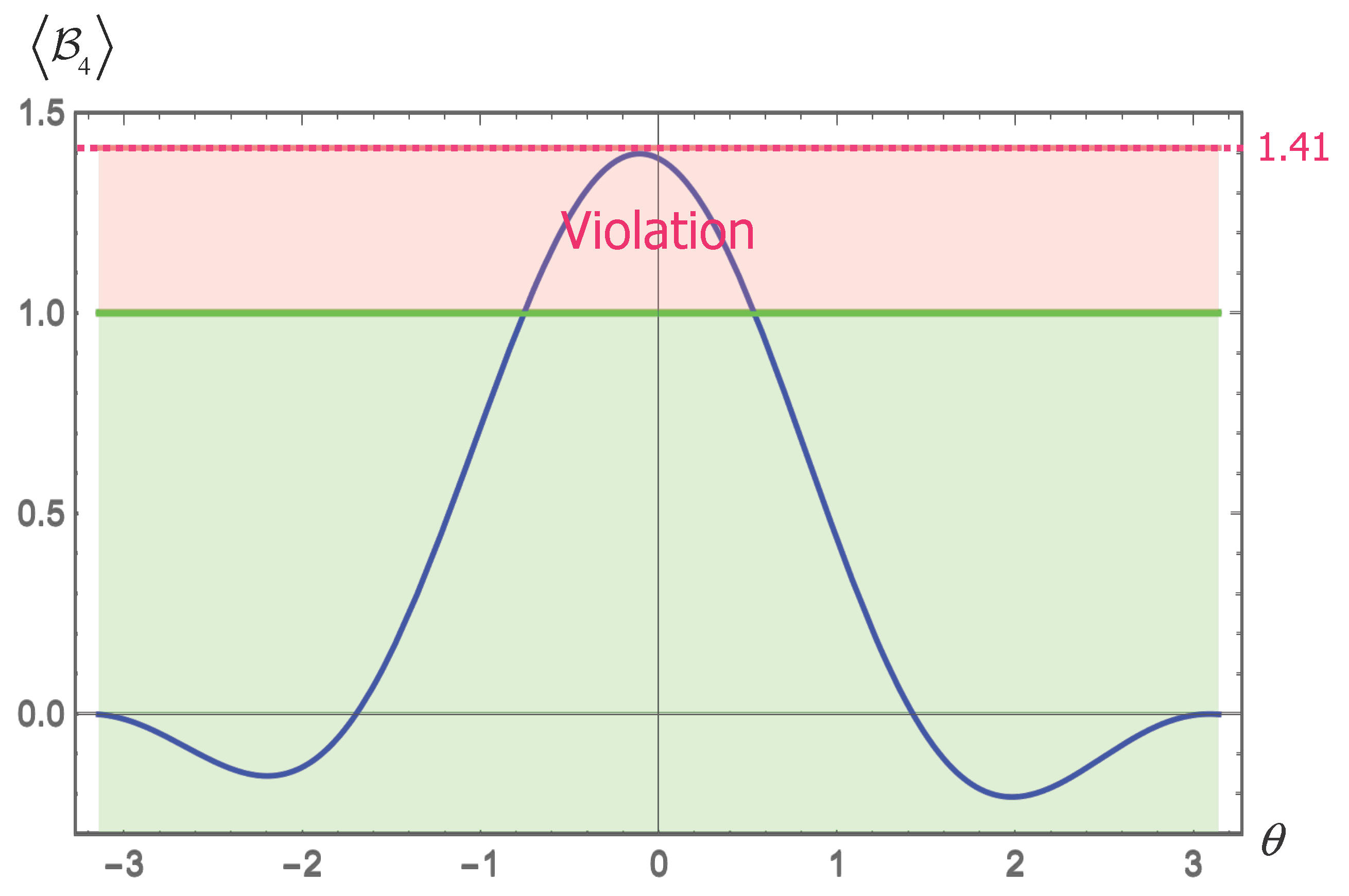
The result is plotted in Figure 2. We see that $\langle {\mathcal{B}}_4\rangle$ is maximally violated but does not exceed $1.41$. Thus, the violation in the BD vacuum does not increase any more, even if we increase the number of modes to measure. This result can be checked by computing

$$\begin{array}{c}\hfill \langle 0_{\mathrm{in}}|{\mathcal{B}}_4|0_{\mathrm{in}}\rangle =\sqrt{1+{tanh}^{2}2r_k}\le \sqrt{2},\end{array}$$

(31)

where Equation (20) is used and $r_k$ is known as the squeezing parameter, defined as

$$\begin{array}{c}\hfill tanh{r}_k=\left|\frac{{\beta }_k}{{\alpha }_k^{*}}\right|=\left|\frac{1}{1-2k^2{\eta }_r^2-2ik{\eta }_r}\right|.\end{array}$$

(32)

Note that $r_k\gg 1$ corresponds to the end of inflation ($k{\eta }_r\ll 1$) and we see that the maximal value is obtained in the infinite squeezing limit $r_k\to \infty$. We also find that the violation does not increase any more, even if we increase the number of modes to measure, say m-pairs $(m=2,3,4\cdots )$. This is in fact a natural consequence of a classification of Bell inequalities in [19,20]. See the details in [9].

4.2. The Case of a Non-Bunch–Davies Vacuum

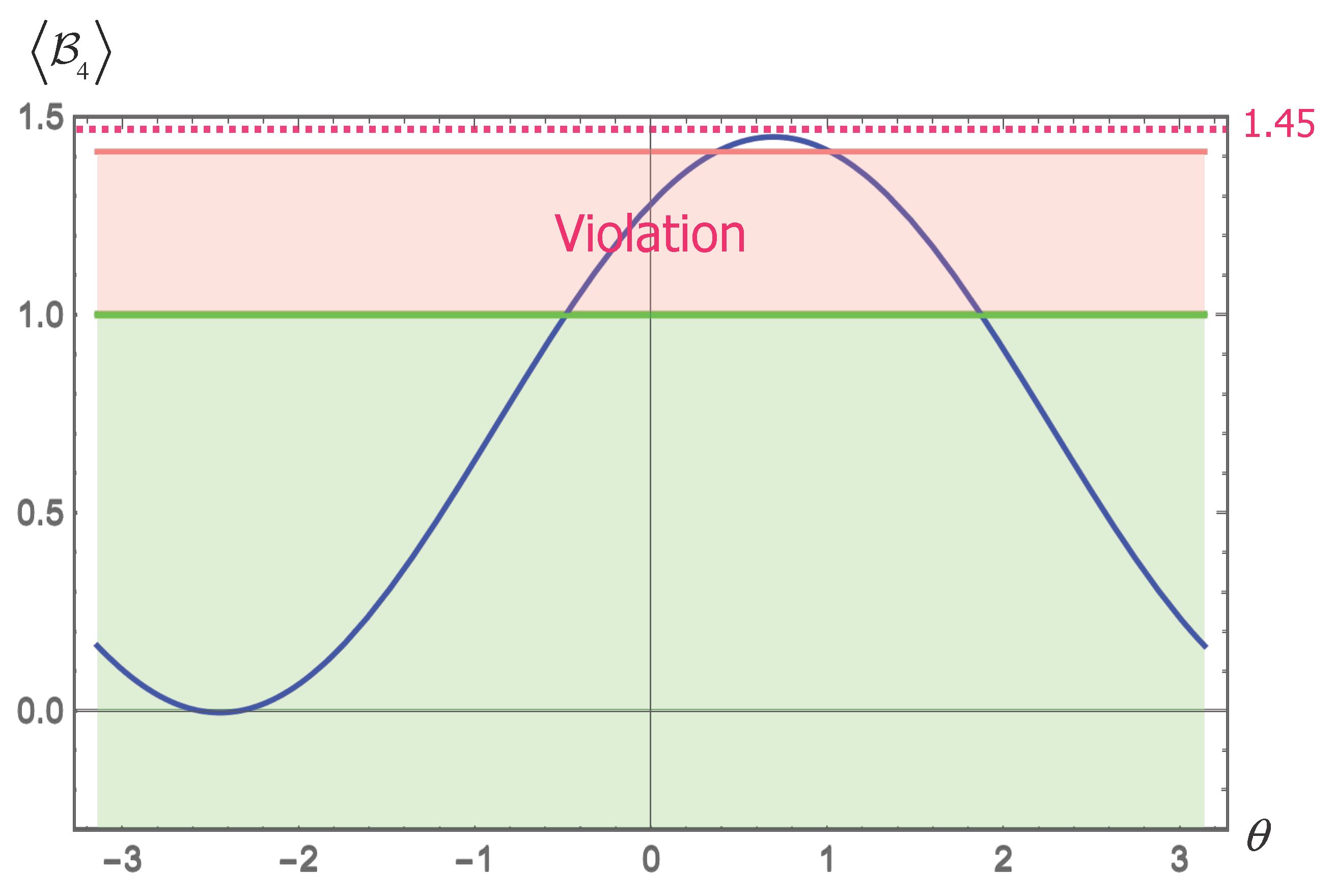
In this case, we get the maximum value $\langle {\mathcal{B}}_4\rangle \sim 1.45$ (see Figure 3), then $q\ge {\left(1.45\right)}^2\simeq 2.1$ and then ${log}_{2}2.1\simeq 1.07>1$. Thus, we have shown that the violation of Bell inequalities increases exponentially with the number of modes to measure k. This indicates that some evidence that our universe has a quantum mechanical origin may survive in CMB data, even if quantum entanglement decays exponentially afterward due to decoherence.

5. Conclusions

We studied the violation of the Bell inequality in initial quantum state of a scalar field in inflation. We showed that the Bell inequality is maximally violated by the Bunch–Davies vacuum. However, it is found that the violation does not increase with the number of modes to measure. On the other hand, we found that the violation increases exponentially with the number of modes to measure for a non-Bunch–Davies vacuum expressed by a four-mode squeezed state of two scalar fields. Our result would be useful to classify the cosmological initial state. These may give rise to the possibility that the evidence that our universe has a quantum mechanical origin may survive in CMB data.

References

- Einstein, A.; Podolsky, B.; Rosen, N. Can quantum mechanical description of physical reality be considered complete? Phys. Rev. 1935, 47, 777. [Google Scholar] [CrossRef]
- Aspect, A.; Grangier, P.; Roger, G. Experimental Tests of Realistic Local Theories via Bell’s Theorem. Phys. Rev. Lett. 1981, 47, 460. [Google Scholar] [CrossRef]
- Aspect, A.; Dalibard, J.; Roger, G. Experimental test of Bell’s inequalities using time varying analyzers. Phys. Rev. Lett. 1982, 49, 1804. [Google Scholar] [CrossRef]
- Maldacena, J. A model with cosmological Bell Inequalities. Fortsch. Phys. 2016, 64, 10. [Google Scholar] [CrossRef]
- Ade, P.A.R.; Aghanim, N.; Arnaud, M.; Arroja, F.; Ashdown, M.; Aumont, J.; Baccigalupi, C.; Ballardini, M.; Banday, A.J.; Barreiro, R.B.; et al. Planck 2015 results. XX. Constraints on inflation. Astron. Astrophys. 2016, 594, A20. [Google Scholar]
- Albrecht, A.; Bolis, N.; Holman, R. Cosmological Consequences of Initial State Entanglement. J. High Energy Phys. 2014, 1411, 093. [Google Scholar] [CrossRef]
- Kanno, S. A note on initial state entanglement in inflationary cosmology. Europhys. Lett. 2015, 111, 60007. [Google Scholar] [CrossRef]
- Kanno, S. Cosmological implications of quantum entanglement in the multiverse. Phys. Lett. B 2015, 751, 316. [Google Scholar] [CrossRef]
- Kanno, S.; Soda, J. Infinite violation of Bell inequalities in inflation. Phys. Rev. D 2017, 96, 083501. [Google Scholar] [CrossRef]
- Bell, J.S. On the Einstein-Podolsky-Rosen paradox. Physics 1964, 1, 195–200. [Google Scholar]
- Clauser, J.F.; Horne, M.A.; Shimony, A.; Holt, R.A. Proposed experiment to test local hidden variable theories. Phys. Rev. Lett. 1969, 23, 880. [Google Scholar] [CrossRef]
- Mermin, N.D. Extreme quantum entanglement in a superposition of macroscopically distinct states. Phys. Rev. Lett. 1990, 65, 1838. [Google Scholar] [CrossRef] [PubMed]
- Belinski, A.V.; Klyshko, D.N. Interference of light and Bell’s theorem. Phys.-Uspekhi 1993, 36, 653–693. [Google Scholar] [CrossRef]
- Werner, R.F.; Wolf, M.M. Bell’s inequalities for states with positive partial transpose. Phys. Rev. A 2000, 61, 062102. [Google Scholar] [CrossRef]
- Alsina, D.; Cervera, A.; Goyeneche, D.; Latorre, J.I.; Życzkowski, K. Operational approach to Bell inequalities: Application to qutrits. Phys. Rev. A 2016, 94, 032102. [Google Scholar] [CrossRef]
- Cirelson, B.S. Quantum Generalizations of Bell’s Inequality. Lett. Math. Phys. 1980, 4, 93. [Google Scholar] [CrossRef]
- Gisin, N.; Bechmann-Pasquinucci, H. Bell inequality, Bell states and maximally entangled states for n qubits. Phys. Lett. A 1998, 246, 1–6. [Google Scholar] [CrossRef]
- Chen, Z.B.; Pan, J.W.; Hou, G.; Zhang, Y.D. Maximal Violation of Bell’s Inequalities for Continuous Variable Systems. Phys. Rev. Lett. 2002, 88, 040406. [Google Scholar] [CrossRef] [PubMed]
- Nagata, K.; Koashi, M.; Imoto, N. Configuration of Separability and Tests for Multipartite Entanglement in Bell-Type Experiments. Phys. Rev. Lett. 2002, 89, 260401. [Google Scholar] [CrossRef] [PubMed]
- Yu, S.; Chen, Z.B.; Pan, J.W.; Zhang, Y.D. Classifying N-Qubit Entanglement via Bell’s Inequalities. Phys. Rev. Lett. 2003, 90, 080401. [Google Scholar] [CrossRef] [PubMed]