Wavepacket Evolution in Unimodular Quantum Cosmology


Faculty of Physics, Gravitational Physics, Boltzmanng. 5, University of Vienna, 1090 Vienna, Austria
Galaxies 2018, 6(1), 8; https://doi.org/10.3390/galaxies6010008
Submission received: 29 November 2017
/
Revised: 29 December 2017
/
Accepted: 3 January 2018
/
Published: 12 January 2018
(This article belongs to the Special Issue Cosmology and the Quantum Vacuum)
Abstract
:The unimodular theory of gravity admits a canonical quantization of minisuperspace models without the problem of time. We derive instead a kind of Schrödinger equation. We have found unitarily evolving wave packet solutions for the special case of a massless scalar field and a spatially flat Friedmann universe. We show that the longterm behaviour of the expectation values of the canonical quantities corresponds to the evolution of the classical variables. The solutions provided in an explicit example can be continued beyond the singularity at , passing a finite minimal extension of the universe.
1. Introduction
The canonical quantization of general relativity leads to the so-called problem of time (see [1] and references therein). In most non-perturbative approaches of quantum gravity time has disappeared from the theory and is seen as an artifact of the classical limit. In contrast to this we will discuss here the quantization of a minisuperspace model in the framework of unimodular gravity. This theory is practically equivalent to general relativity at the classical level, but since it has a different canonical structure time does not disappear from the quantum theory [2]. Investigations of unimodular quantum cosmology can be found in [3,4] as well as more recently in [5] where unimodular quantum loop cosmology is discussed. In [4] a semiclassical wave function via path integral for an empty universe with positive curvature is constructed. The time evolution fails to be unitary. The model mentioned in [3] is the spatially flat universe with a massless scalar field. Here the general solution is given only formally, and the properties of the wave packet evolution in particular the question of unitary time evolution are not discussed. The solutions in [5] apply for a flat universe filled with exotic matter with the equation of state .
In this article we consider the quantization of spatially flat universe with a massless scalar field. We construct a class of unitarily evolving solutions with a negative expectation value of the Hamiltonian (that correspond classically to an infinitely expanding universe). Based on an example we investigate the time evolution of characteristic expectation values and compare it to the classical dynamics.
2. Unimodular theory
The Einstein-Hilbert action of general relativity is given by
where
contains the velocity of light c and the gravitational constant G. The second integral is defined on the spacelike boundary of the considered space-time region . The space-time metric with induces a three-dimensional metric with on the boundary . The corresponding second fundamental form is denoted by with the trace K. If we also take into account the matter action that describes the fields, the variation of with respect to the metric yields the Einstein equations.
where the energy-momentum tensor is given by
If we start instead with an Einstein Hilbert action (1) with and vary it under the restriction , we obtain Einsteins equations with an arbitrary additional constant , that can be identified with the cosmological constant of general relativity [2].
This theory is called unimodular gravity. Any solution of unimodular gravity (4) is also a solution of general relativity (2) for a specific cosmological constant and vice versa. The only difference between the two theories is, that is a natural constant in general relativity while it is a conserved quantity in unimodular gravity. But since in both theories the cosmological constant can not vary over the whole universe, we would have to investigate different universes to determine if solutions with different exist (unimodular theory) or if is a “true” natural constant. So the two theories are practically indistinguishable. Nevertheless the canonical structure of the theories differs [2] and therefor the quantization of unimodular theory yields different results compared to the quantization of general relativity [3]. In this article we will confine the discussion of the canonical structure to the minisuperspace model we wish to quantize.
3. The Spatially Flat Friedmann Universe with a Scalar Field in Unimodular Theory
The metric of a homogeneous and isotropic spacetime (Friedmann universe)
is characterized by the lapse function N(t) and the scale factor . If the spatial curvature is zero, is the line element of three-dimensional flat space.
Inserting the metric into the Einstein-Hilbert action (1) with yields [1]
where is is the volume of the spacelike slices according to (5).
The action of a scalar field in curved spacetime reads
If
the variation with respect to yields the Klein-Gordon equation for a particle with mass
Since we consider a spatial homogeneous spacetime, the spatial derivatives of the field must be zero. Inserting (5), we find
Therefore the Lagrange function reads
where we have introduced the abbreviation . If we incorporate into the variables a and N as well as
we find for the rescaled Lagrangian
According to unimodular theory the lapse function (13) is determined by and the Friedmann metric (with unscaled quantities) has the form
Since the condition is not influenced by the scaling (10) we find for the rescaled unimodular Lagrange function (11)
The momenta conjugate to the variables a and read
We obtain for the Hamiltonian of the unimodular theory
The Hamiltonian is a conserved quantity. If we write the Hamiltonian as a function of the configuration variables and their derivatives
we find that
equals the Hamiltonian constraint of general relativity for . We see that this special labeling of the conserved quantity makes the solutions of unimodular gravity and general relativity coincide (see Appendix A). Nevertheless the Hamiltonian according to general relativity differs from (15).
4. Classical Solutions of a Flat Friedmann Universe with a Massless Scalar Field
The simplest case of a matter Lagrangian is , which would correspond to the field of a massless particle with spin zero (7). If instead a perfect fluid matter model is chosen, the solutions for a massless scalar field can be shown to be equivalent to the solutions for the special case of stiff matter (see [6]).
The Hamiltonian reads
According to the equations of motion is a conserved quantity
and the time-dependence of the field is given by
If we assume , we obtain the de-Sitter solutions with . The conservation of the Hamiltonian
implies
We then find for the scale factor
Note that this solution of unimodular theory coincides with a solution of general relativity with a choice of coordinates with in (5).
If ,
yields
We obtain
where Z is an integration constant that determines . For the scale factor we have assumed .
5. Quantization of a Flat Friedmann Universe with a Massless Scalar Field
The canonical quantization of the unimodular Hamiltonian of the model (17) yields for the massless case ()
Here we have chosen the factor ordering that gives the part of the Hamiltonian that is quadratic in the momenta the form of a Laplace Beltrami operator [1].
The evolution of the wavefunction is determined by
The Hamiltonian is symmetric with respect to the inner product defined by the measure , where and .
With the transformation
and the volume element , the Hamiltonian assumes the form
This expression has the appearance of the wave equation in polar coordinates, which shows that our minisuperspace is flat. The Hamilton operator equals the wave operator in Rindler spacetime. We bring the Hamiltonian into the simplest form using a transformation to light-cone coordinates:
We obtain the Hamiltonian
The volume element is given by and , . This is equivalent to a volume element , if the wave functions are accordingly normalized. We will search for solutions of ( 23) that are square integrable. Moreover they should fulfill the condition for a unitary time evolution that is given by
For this condition ensures that the norm of the wavepackets is preserved:
Differentiating (27) with respect to results in the conservation of the expectation value of the Hamiltonian
Higher time derivatives yield
6. Solutions with a Negative (Expectation) Value of the Hamiltonian
This equation looks rather simple and there are many possibilities to solve it. The challenge here is to find solutions that ensure a unitary time evolution. We will obtain this goal by a superposition of eigensolutions. An eigenstate with negative eigenvalue fulfills the equation
which gives the time-dependent solution
The Laplace transformation (see f.i. [7]) of (33) with respect to v yields
where is given by
and we have used the differential rule of the Laplace transform [7] Solving (35), we obtain
Applying the formula for the inverse Laplace transform (see [8])
and the convolution theorem [7] we find for the inverse Laplace transform
The functions determine at the edges
The superposition of the corresponding eigensolutions (34) yields more general time-dependent wavepacket solutions of (32)
The solution is then characterized by the functions . We assume that they can be chosen appropriately to ensure that is square integrable. We obtain for the time evolution at the edges
which means that (37) meets the condition (30) for a unitary time evolution if are real functions. Moreover it follows from the Riemann-Lebesgue lemma (see for instance [7]) for the Fourier transform that
if is an absolutely integrable function. This implies for the wavefunction at the edges
It will turn out to be more convenient to represent as
The initial wavefunction then reads
This is a consequence of the selfreproducing property of the Hankel transformation [7]
which is equivalent to
7. Example for a Wavepacket Evolution with a Negative Expectation Value of the Hamiltonian
In Section 6 we constructed solutions of (32) with a negative expectation value of the Hamiltonian and a unitary time evolution. We had to require that the functions ensure that the initial wave function (42) is square integrable. Investigating an explicit example shows that an appropriate choice of these functions is possible. The lengthy algebraic calculations of this section were performed with Wolfram Mathematica.
We define
With the additional real parameters and , we find for the initial function according to (42)
where we have introduced a normalization factor that turns out to be
We obtain for the expectation value of the Hamiltonian
The time evolution of is determined by (44):
We find for the late phase of the time evolution (where we have replaced by t (31)):
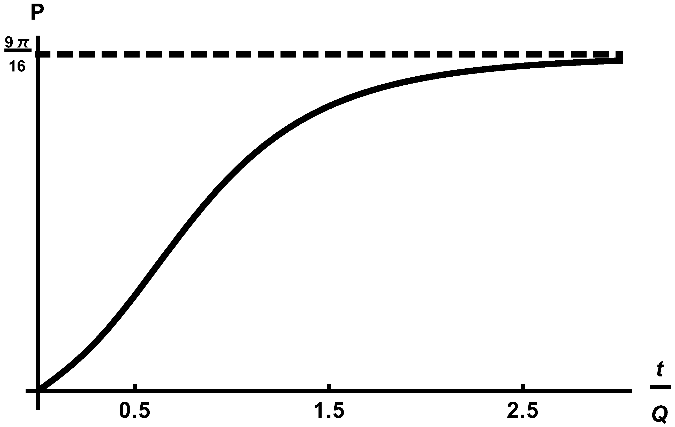
which coincides with the classical behaviour according to (21a). We also find that the expectation value of approaches a constant value
which shows that the classically conserved quantity is only a constant of motion in the late phase of time evolution (see Figure 1).
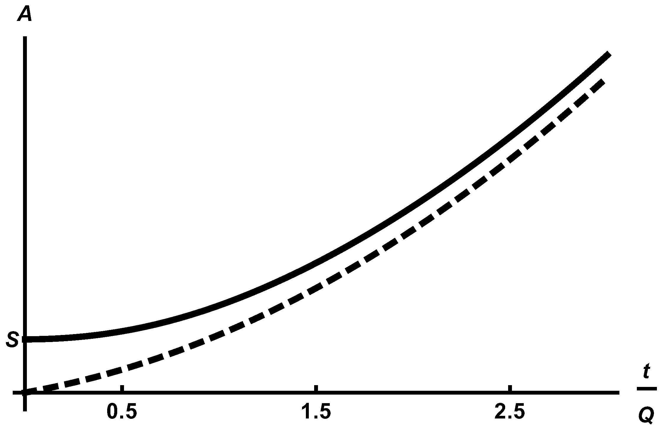
Nevertheless at the beginning of the time evolution, the observable that is proportional to the sixth power of the scale factor assumes a constant value Figure 2.
We can also prove that the linear part of the classical time evolution of (21a) is reproduced by the late time behaviour of the expectation value. Inserting for (51), we find
which shows that the time evolution of the expectation value approaches the classical evolution (see Figure 2). For the variance of we find
which yields
8. Discussion and Conclusions
It is important to note that the system behaves more and more classically at late times. An approximate classical behaviour far away from the singularity was also predicted for the case of exotic matter in [5]. This is in contrast to quantum mechanics, where systems start with classical motion developing quantum properties in the late phase of time evolution, as the revival phenomena show impressively (see f.i. [10]). However this classical behaviour for late times does not apply to all aspects of the time evolution because the uncertainty of the observable , that is related to the scale factor increases with time. We think that this would not happen with a more realistic matter model.
The construction of solutions according to (37) also works for negative times and so the solutions can be continued beyond the classical singularity at . In the special case we investigated (50) this would yield a contracting universe that passes a minimal extension before expanding again. The question of solutions with a positive expectation value of the Hamiltonian remains open. Moreover we think that unimodular quantum gravity gives the opportunity to investigate effects of cosmological evolution (as inflation, acceleration of the expansion universe) in the framework of a quantum theory of gravity without being confined to a semiclassical limit.
Acknowledgments
I thank Helmut Rumpf for calling my attention to unimodular gravity. I thank Christiane Lechner for proposing the transformation to light cone coordinates that helped me to analyze the minisuperspace equation of unimodular quantum cosmology.
Conflicts of Interest
The author declares no conflict of interest.
Appendix A. Hamiltonian Constraint According to General Relativity
Inserting the metric (5) into the Einstein-Hilbert action with cosmological constant yields
The variation of (A2) with respect to N yields
This equation establishes a relation of the variables and their first derivatives. It represents the Hamiltonian constraint of general relativity and equals (16) for . Nevertheless the Hamiltonian differs from the respective expression in the canonical quantization of general relativity with cosmological constant (see also [11])
References
- Kiefer, C. Quantum Gravity; Oxford University Press: Oxford, UK, 2012. [Google Scholar]
- Henneaux, M.; Teitelboim, C. The cosmological constant and general covariance. Phys. Lett. B 1989, 222, 195–199. [Google Scholar]
- Unruh, W.G. Unimodular theory of canonical quantum gravity. Phys. Rev. D 1989, 40, 1048–1051. [Google Scholar] [CrossRef]
- Daughton, A.; Louko, J.; Sorkin, R.D. Initial conditions and unitarity in unimodular quantum cosmology. arXiv, 1993; arXiv:gr-qc/9305016. [Google Scholar]
- Chiou, D.; Geiller, M. Unimodular loop quantum cosmology. Phys. Rev. D 2010, 82, 064012. [Google Scholar] [CrossRef]
- Masden, M.S. A note on the equation of state of a scalar field. Astrophys. Space Sci. 1985, 113, 205–207. [Google Scholar]
- Zayed, A. Handbook of Function and Generalized Function Transformations; CRC Press: Boca Raton, FL, USA, 1996. [Google Scholar]
- Erdely, A. Tables of Integral Transforms; McGraw-Hill Book Company: New York, NY, USA, 1954. [Google Scholar]
- Magnus, W.; Oberhettinger, F.; Soni, R.P. Formulas and Theorems for the Special Functions of Mathematical Physics; Springer: Berlin/Heidelberg, Germany, 1966. [Google Scholar]
- Robinett, R. Quantum wave packet revivals. Phys. Rep. 2004, 392, 1–119. [Google Scholar] [CrossRef]
- Craig, C.A.; Singh, P. Consistent probabilities in Wheeler-De Witt quantum cosmology. Phy. Rev. D 2010, 82, 123526. [Google Scholar] [CrossRef]
Figure 1.
The quantity converges to . We have chosen , and time is scaled by .

© 2018 by the author. Licensee MDPI, Basel, Switzerland. This article is an open access article distributed under the terms and conditions of the Creative Commons Attribution (CC BY) license (http://creativecommons.org/licenses/by/4.0/).
Share and Cite
MDPI and ACS Style
Riahi, N. Wavepacket Evolution in Unimodular Quantum Cosmology. Galaxies 2018, 6, 8. https://doi.org/10.3390/galaxies6010008
AMA Style
Riahi N. Wavepacket Evolution in Unimodular Quantum Cosmology. Galaxies. 2018; 6(1):8. https://doi.org/10.3390/galaxies6010008
Chicago/Turabian StyleRiahi, Natascha. 2018. "Wavepacket Evolution in Unimodular Quantum Cosmology" Galaxies 6, no. 1: 8. https://doi.org/10.3390/galaxies6010008
Note that from the first issue of 2016, this journal uses article numbers instead of page numbers. See further details here.