An Arbitrary Lagrangian–Eulerian Formulation for Modelling Cavitation in the Elastohydrodynamic Lubrication of Line Contacts

Abstract

In this article an arbitrary Lagrangian–Eulerian (ALE) formulation for modelling cavitation in elastohydrodynamic lubrication (EHL) is derived and applied to line contact geometry. The method is developed in order to locate the position of cavitation onset along the length of the contacting region which gives the transition from liquid to vapour in the fluid. The ALE is implemented by introducing a spatial frame of reference in which the solution is required and a material frame of reference in which the governing equations are solved. The spatial frame is moved from the material frame according to the error in the Neumann pressure gradient constraint required at the cavitation location when Dirichlet constraints are imposed for pressure in the liquid phase. Results are calculated under both steady-state and transient operating conditions using a multigrid solver. The solutions obtained are compared to established literature and conventional approaches to modelling cavitation which show that the ALE formulation is an alternative, straightforward and accurate means of implementing such conditions in EHL. This is achieved without the penalties associated with the numerical modelling of Heaviside functions or free boundaries.

1. Introduction

Elastohydrodynamic lubrication (EHL) considers two bodies rotating under load in fully-flooded conditions in which pressure generated in the lubricant subsequently causes deformation of the bounding surfaces, this interaction is fully-coupled to reach a load-carrying capacity for the contact [1]. The solution to the EHL problem is well-established whereby the fluid flow and solid deformation are accurately described by the Reynolds equation and Hertzian contact mechanics respectively. The lubricant also exhibits compressibility and piezoviscosity, which contributes to the pressure generated in the contact [2]. However because the lubricant (as a liquid) cannot hold a large tensile stress, when the pressure is low the fluid film will rupture and air trapped in the lubricant will vapourise, forming bubbles [3]. This phenomena is known as hydrodynamic cavitation and has a significant impact on the lubrication. In regions of the contact where fluid is vapourised, pressure can be considered constant and takes a value known as the saturated vapour pressure (or cavitation pressure). The saturated vapour pressure is similar in magnitude to ambient pressure but very small when compared to the contact pressure. Authors have sought solutions to the problem of cavitation by representing experientially observed fluid flow behaviour in the Reynolds equation, the most significant development of these is the Jakobsson–Floberg–Olsson (JFO) cavitation boundary conditions [4,5,6]. These conditions describe that hydrodynamic cavitation occurs in the outlet region of a lubricated contact and that for the fluid flow to remain mass conservative both the pressure and pressure gradient must be equal to zero.

The works of Ertel [7] and Grubin [8] were significant in providing the first EHL solutions giving the correct magnitudes of pressure and film thickness. These calculations used an inverse method in which the domain was split in two, the inlet (low pressure) region was solved using a forward iterative scheme and for the outlet (high pressure) region a film shape was assumed from which the pressure distribution was determined. The algorithm continued until convergence in pressure at the crossover point was observed. Due to the way in which the pressure distribution was calculated, cavitation was satisfied automatically by the algorithm. Dowson and Higginson [9] later established solutions to the full EHL problem using a forward iterative method. In this approach the fluid flow equations were solved for pressure using a Gauss–Seidel numerical scheme in which cavitation was treated by specifying pressure to zero whenever a negative value was intermediately observed in the solution procedure. Cavitation onset and the solution to the JFO conditions were therefore treated as a free boundary problem.

The forward iterative method of Dowson and Higginson [9] made accurate predictions but took a very long time to compute and performed ineffectively at high loads. It was for this reason that multilevel methods for EHL were developed, the works of Venner [10] and Venner and Lubrecht [11] on the subject outline in detail this numerical procedure. Using these techniques and the same treatment for cavitation as implemented by the forward iterative method the authors were able to solve EHL contact problems over a wide range of operating conditions and material properties. More recently Habchi et al. [12] developed a fully-coupled method for EHL from which very high pressures can be achieved. In this approach elastic deformation was considered by replacing the Hertzian contact approach with a three-dimensional body calculation, with the fluid phase and cavitation modelled using the same approach as employed by multilevel methods. Wu [13] also developed a method for modelling cavitation in EHL, which employed a penalty formulation as part of the numerical algorithm.

In the calculation of EHL problems described thus far, cavitation was modelled as part of the solution procedure in which pressure was forced to be positive and the JFO conditions were sought after in the resulting distributions. This adds to the complex non-linear nature of the problem and causes numerical difficulties when solving the governing equations due to the additional constraints brought by cavitation. The JFO conditions were implemented in a different way by Elrod [14], who derived a universal mass-conserving equation for the liquid and vapour pressure and the subsequent finite element (FE) scheme. Vijayaraghavan and Keith [15] generalised these results and both are frequently used to study the effects of cavitation in a range of applications. Elrod’s approach assumed an incompressible fluid and no solid deformation, with the bulk modulus of the lubricant used to couple density in the liquid and vapour phases [14]. Bayada et al. [16,17,18] developed the method for including elastohydrodynamic effects and the influence of homogenised surface roughness, and subsequently Sahlin et al. [19] generalised the method for arbitrary pressure–density relationships.

Recently progress has also been made in the mathematical modelling of cavitation in hydrodynamic lubrication by Giacopini et al. [20], who reformulated the model of Bayada et al. [16,17] into one which can be solved as a linear complementary problem using well-established numerical methods. The idea of complementarity was extended by Bertocci et al. [21] who formulated a nonlinear complementary problem and by Fan and Behdinan [22] to investigate squeeze film damper problems. Almqvist et al. [23] used a different approach in which the pressure–density relationship is not substituted into the Reynolds equation but instead derived by investigating the conservation of mass in both the liquid and vapour phases before considering complementarity. The work of Almqvist et al. [23] covers compressible fluids and was extended by Almqvist and Wall [24] for generalised pressure–density and pressure–viscosity relationships.

Calculations made using algorithms based on Elrod [14] are commonplace and depend greatly on the magnitude of the liquid bulk modulus, in which round-off errors can readily be generated owing to the stiffness of the governing equations. It is often practical to implement a lower-than-representative value in order to improve numerical convergence. Yang and Keith [25] discuss this practicality in application to deriving a cavitation algorithm for piston ring lubrication including generalised liquid compressibility. Authors are actively researching with the aim of improving the effectiveness of the Elrod model in particular applications. Miraskari et al. [26] modified the model for robust predictions of cavitation in journal bearings, Rothwell et al. [27] changed the approach for the thermal analysis of highly loaded journal bearings, Garcia et al. [28] developed the method for modelling piezoviscosity in hydrodynamic lubrication and Woloszynski et al. [29] adapted the solution algorithm for fast computations. The Elrod approach is attractive because of the simplicity and accuracy of the method for modelling cavitation related phenomena and it is for this reason that work remains of interest in the study of lubrication. However the problems associated with modelling discontinuous Heaviside functions underpinning the approach remain and authors have sought different solutions.

Cavitation is a two-phase flow phenomenon and as such authors have derived models based on a volumetric or void fraction. This is conventionally defined by the ratio of phase densities in a given volume and is subsequently used to establish fluid flow transport equations. Kumar and Booker [30] derived a solution for two-phase flow in journal bearings which modifies the Elrod model [14] and is a widely cited cavitation algorithm. Grando et al. [31] developed a two-phase model for journal bearings by considering the interaction between liquid and gas properties and phase dissolution. Bayada and Chupin [32], Bruyere et al. [33], and van Odyck and Venner [34] have all developed models investigating two-phase flows in lubricated contacts. These approaches avoid the problems associated with modelling discontinuous functions or free boundaries. However they require fine grid sizes and significant progress is needed to capture the transition between phases accurately. For example, see the recent work of van Emden et al. [35,36], who developed a numerical model of bubble formation in the outlet flow of an elastohydrodynamically lubricated contact.

Another type of two-phase model are those based on computational fluid dynamics (CFD). These problems do not necessarily rely on the Reynolds equation and as such cavitation is not considered by the JFO conditions. Instead CFD solutions consider the transport of mass, momentum and energy in both phases. Bruyere et al. [37] derived a CFD approach to thermal EHL problems that employed a density variation to couple the liquid and vapour phases. Hartinger et al. [38] solved CFD problems for EHL line contacts under shear-thinning and thermal conditions, which was further developed by Hajishafiee et al. [39] to operate over a wider range of operating conditions and contact pressures. In [38,39], the authors derive a solution to the EHL problem by solving the Navier–Stokes and energy equations with elastic deformation, and subsequently consider cavitation by means of a method developed by Kärrholm et al. [40] for isentropic phase change. CFD provides interest for EHL problems due to the difference assumptions between such models and the Reynolds approach. However, in comparison, the simplicity and accuracy of Reynolds-based models (with cavitation treated using the JFO conditions) means that they remain of significant importance.

In the modelling of JFO cavitation boundary conditions, the authors either use Heaviside functions in their derivations in order to determine the onset of cavitation and adapt the governing equations accordingly; or adapt the solution procedure to force pressure to be positive and subsequently solve for cavitation onset. The resulting formulations are continuous due to switching between liquid and vapour phases and the corresponding mass-conservative descriptions of fluid transport. Since these models rely on Heaviside functions or free boundaries to determine the onset of cavitation there is a penalty associated with the numerical calculation of pressure. This is in addition to the complex mechanics which describe EHL and overall leads to a series of mathematically stiff non-linear differential equations which are challenging to solve. This research continues to be published in the field of cavitation modelling in EHL, and as such authors are constantly trying to improve these methods. In the present work we derive an alternative solution to the JFO conditions in EHL that does not rely on such assumptions and instead obtains the onset of cavitation as part of the solution procedure.

This article formulates an arbitrary Lagrangian–Eulerian (ALE) method [41] to model the JFO cavitation boundary conditions in EHL. For this purpose, two frames of reference are defined: (i) a material (stationary) frame in which the governing equations are solved; and (ii) a spatial (moving) frame in which the governing equations are derived. The ALE is used to relate the material and spatial frames by implementing a moving component, this motion is determined based on the pressure gradient calculated at the location where cavitation is onset. The liquid and vapour phases are modelled using different governing equations and the solutions obtained are continuous and mass-conservative. Schweizer [42] developed an ALE formulation for modelling cavitation in hydrodynamic lubrication and applied the method to three-dimensional journal bearings under steady-state, linearly compressible and isoviscous conditions. In this paper we derive a new method for investigating EHL in line contacts based on similar principles, which additionally considers transients, arbitrary pressure–density and arbitrary pressure–viscosity relationships. Authors have also developed ALE formulations for thin film flow problems with moving boundaries, such as those found in the modelling of menisci [43] and free surfaces [44]. The main advantage to the method introduced is the simplicity in which the solution to pressure in both phases can be obtained, as calculated using a commercial software package. The formulation does not rely on any switching and as such cavitation onset is determined without the numerical sensitivity associated with modelling Heaviside functions or free boundary problems. It can therefore been seen as an efficient and effective means of modelling the JFO boundary conditions in EHL.

2. Materials and Methods

2.1. Theoretical Formulation

In this subsection the relevant theory applicable to EHL is outlined, subsequently the solution to the JFO cavitation boundary conditions using an ALE formulation is derived.

2.1.1. Elastohydrodynamic Lubrication

In this article the EHL of a line contact is considered in which two cylindrical bodies with given radii ${\mathrm{R}}_1,{\mathrm{R}}_2$ come into contact under fully-flooded conditions. The bodies rotate about their origins along their line of symmetry and result in the surface velocities ${\mathrm{U}}_1,{\mathrm{U}}_2$ in the sliding direction $\mathrm{x}$ at the contacting interface, as they come into contact pressure $\mathrm{p}$ is generated in the lubricant, which in turn causes deformation of the bounding surfaces. This deformation is characterised by the elastic properties of the solid materials: the Young’s moduli ${\mathrm{E}}_1,{\mathrm{E}}_2$ and Poisson ratios ${\mathsf{\nu }}_1,{\mathsf{\nu }}_2$. Subsequently the surfaces become separated by a thin film of thickness $\mathrm{h}$ and in order to reach a load carrying capacity $\mathrm{w}$ the contact separation ${\mathrm{h}}_0$ must be determined. As per convention the Hertzian contact pressure ${\mathrm{p}}_{\mathrm{h}}$ and half-width $\mathrm{b}$ are used to non-dimensionalise the governing equations and from herein an overbar notation is used for all variables. A nomenclature is provided in Appendix A.

An example sketch for the pressure and film thickness distributions in an EHL line contact are shown in Figure 1. The domain is described in one-dimension by $\overline{\mathrm{x}}$ and is separated into two distinct regions ${\mathsf{\Omega }}_1$ and ${\mathsf{\Omega }}_2$, in ${\mathsf{\Omega }}_1$ the lubricant is liquid and in ${\mathsf{\Omega }}_2$ the lubricant is vapour. The domains are bounded by the upstream $\overline{{\mathrm{x}}_{\mathrm{u}}}$, downstream $\overline{{\mathrm{x}}_{\mathrm{d}}}$ and cavitation $\overline{{\mathrm{x}}_{\mathrm{c}}}$ locations, see Equation (1).

$${\mathsf{\Omega }}_1=\left\{\left(\overline{\mathrm{x}}\right)|\overline{{\mathrm{x}}_{\mathrm{d}}}\le \overline{\mathrm{x}}\le \overline{{\mathrm{x}}_{\mathrm{c}}}\right\}{\mathsf{\Omega }}_2=\left\{\left(\overline{\mathrm{x}}\right)|\overline{{\mathrm{x}}_{\mathrm{c}}}\le \overline{\mathrm{x}}\le \overline{{\mathrm{x}}_{\mathrm{u}}}\right\}$$

(1)

In terms of hydrodynamics, the liquid phase is governed by the Reynolds equation and in the vapour phase pressure is equal to the saturated vapour pressure; subject to the JFO cavitation boundary conditions this provides a sufficient description for mass conservation in the fluid. For the liquid phase ${\mathsf{\Omega }}_1$ the non-dimensional Reynolds equation is written for pressure as according to Equations (2) and (3):

$$\frac{\partial }{\partial \overline{\mathrm{x}}}\left(\mathsf{\epsilon }\frac{\partial \overline{\mathrm{p}}}{\partial \overline{\mathrm{x}}}\right)=\frac{\partial \left(\overline{\mathsf{\rho }}\overline{\mathrm{h}}\right)}{\partial \overline{\mathrm{x}}}+\frac{\partial \left(\overline{\mathsf{\rho }}\overline{\mathrm{h}}\right)}{\partial \overline{\mathrm{t}}}$$

(2)

$$\mathsf{\epsilon }=\frac{{\overline{\mathsf{\rho }}\overline{\mathrm{h}}}^3}{\mathsf{\lambda }\overline{\mathsf{\eta }}}\mathsf{\lambda }=\frac{12{\mathrm{U}}_{\mathrm{m}}{\mathsf{\eta }}_0{\mathrm{R}}^2}{{\mathrm{p}}_{\mathrm{h}}{\mathrm{b}}^3}$$

(3)

where $\overline{\mathrm{p}}$ is the pressure, $\overline{\mathrm{h}}$ is the film thickness, $\overline{\mathrm{t}}$ is time, $\overline{\mathsf{\rho }}$ is the fluid density, $\overline{\mathsf{\eta }}$ is the fluid viscosity, ${\mathsf{\eta }}_0$ is the viscosity at ambient pressure, ${\mathrm{U}}_{\mathrm{m}}$ is the entrainment velocity and $\mathrm{R}$ the reduced contact radius. In EHL it is known that the fluid density and viscosity vary strongly with pressure, in order to demonstrate that any such relationship can be used in this method example relationships have been selected. The pressure–density varies as according to Dowson and Higginson [45] and the pressure–viscosity varies as according to Roelands [46]. See Equations (4) and (5) respectively:

$$\overline{\mathsf{\rho }}=\frac{{\mathrm{D}}_0/{\mathrm{p}}_{\mathrm{h}}+{\mathrm{D}}_1\overline{\mathrm{p}}}{{\mathrm{D}}_0/{\mathrm{p}}_{\mathrm{h}}+\overline{\mathrm{p}}}$$

(4)

$$\overline{\mathsf{\eta }}=\exp \left(\ln \left(\frac{{\mathsf{\eta }}_0}{{\mathsf{\eta }}_{\mathrm{r}}}\right)\left[{\left(1+\frac{{\mathrm{p}}_{\mathrm{h}}\overline{\mathrm{p}}}{{\mathrm{p}}_{\mathrm{r}}}\right)}^{\mathrm{Z}}-1\right]\right)$$

(5)

where ${\mathrm{D}}_0,{\mathrm{D}}_1,{\mathrm{p}}_{\mathrm{r}},{\mathsf{\eta }}_{\mathrm{r}}$ and $\mathrm{Z}$ are material constants for a specific lubricant.

The solution to Reynolds equation in ${\mathsf{\Omega }}_1$ is obtained by specifying ambient pressure downstream (Equation (6)) and the JFO cavitation boundary conditions at the cavitation location (Equations (7)):

$$\overline{\mathrm{p}}\left(\overline{{\mathrm{x}}_{\mathrm{d}}}\right)=0$$

(6)

$${\frac{\partial \overline{\mathrm{p}}}{\partial \overline{\mathrm{x}}}|}_{\overline{{\mathrm{x}}_{\mathrm{c}}}}=0\hspace{1em}\overline{\mathrm{p}}\left(\overline{{\mathrm{x}}_{\mathrm{c}}}\right)=\overline{{\mathrm{p}}_{\mathrm{c}}}$$

(7)

where $\overline{{\mathrm{p}}_{\mathrm{c}}}$ is the saturated vapour pressure. This is known to be similar in magnitude to the ambient pressure and very small compared to the contact pressure, therefore the condition of $\overline{{\mathrm{p}}_{\mathrm{c}}}=0$ is implemented such that pressure is always greater than zero in the liquid phase.

Pressure in ${\mathsf{\Omega }}_2$ is determined by the saturated vapour pressure (Equations (8)) and is specified by definition of the cavitation location $\overline{{\mathrm{x}}_{\mathrm{c}}}$:

$$\overline{\mathrm{p}}=\overline{{\mathrm{p}}_{\mathrm{c}}}$$

(8)

However, knowing the location at which this pressure is reached cannot be determined prior to the analysis and because of the coupling between Dirichlet and Neumann type constraints in Equation (7), cavitation becomes a complex numerical problem to solve. It is for this reason that cavitation algorithms and the universal cavitation equation were developed, in this article we derive an ALE formulation for this purpose as outlined in Section 2.1.2.

The film thickness is determined by considering Hertizan contact mechanics in order to describe the elastic deformation of the bodies under load, see Equation (9):

$$\overline{\mathrm{h}}=\overline{{\mathrm{h}}_0}+\frac{{\overline{\mathrm{x}}}^2}{2}-\frac{1}{\mathsf{\pi }}\underset{\overline{{\mathrm{x}}_{\mathrm{d}}}}{\overset{\overline{{\mathrm{x}}_{\mathrm{c}}}}{{\displaystyle \int }}}{\overline{\mathrm{p}}}^{\prime }\ln \left|\overline{\mathrm{x}}-{\overline{\mathrm{x}}}^{\prime }\right|\mathrm{d}{\overline{\mathrm{x}}}^{\prime }$$

(9)

The minimum film thickness $\overline{{\mathrm{h}}_{\min }}$ represents the lowest value of $\overline{\mathrm{h}}$ in the contacting region, it is of note that this does not necessarily occur at the same location as $\overline{{\mathrm{x}}_{\mathrm{c}}}$. The last term of Equation (9) represents elastic deformation of the bounding surfaces and is conventionally calculated using a stiffness matrix. In which, at any location in the contact, the influence to deformation diminishes with distance from the applied load and through superposition describes the convolution.

The load capacity is described by Equation (10) and is satisfied by varying the contact separation $\overline{{\mathrm{h}}_0}$, where ${\mathrm{C}}_{\mathrm{w}}$ is the dynamic loading coefficient:

$$\underset{\overline{{\mathrm{x}}_{\mathrm{d}}}}{\overset{\overline{{\mathrm{x}}_{\mathrm{c}}}}{{\displaystyle \int }}}\overline{\mathrm{p}}\mathrm{d}\overline{\mathrm{x}}={\mathrm{C}}_{\mathrm{w}}\frac{\mathsf{\pi }}{2}$$

(10)

Additionally, since $\overline{{\mathrm{p}}_{\mathrm{c}}}=0$, the integral functions of Equations (9) and (10) are truncated about the cavitation location and represent integration on ${\mathsf{\Omega }}_1$ alone, this is because there is no influence of pressure from these functions in ${\mathsf{\Omega }}_2$.

2.1.2. Arbitrary Lagrangian–Eulerian Formulation

The JFO cavitation boundary conditions specify both Dirichlet (value-based) and Neumann (gradient-based) type constraints for pressure at the cavitation location $\overline{{\mathrm{x}}_{\mathrm{c}}}$, therefore this location must be identified as part of the solution procedure in order to meet the requirements for mass-conservation. For this purpose an ALE formulation is derived in which the coordinate direction $\overline{\mathrm{x}}$ is considered to be part of a spatial (moving) frame of reference and the coordinate direction $\overline{\mathrm{X}}$ is introduced in a material (stationary) frame of reference. The spatial frame of reference is that in which the governing equations are derived and the material frame of reference is that in which the equations are solved. The spatial coordinates $\overline{\mathrm{x}}$ become an additional variable which must be solved for along with those governing EHL, all variables and functions are updated accordingly with respect to the material coordinates $\overline{\mathrm{X}}$.

For the ALE formulation the material frame of reference represents initial domains ${{\mathsf{\Omega }}_1}^{\prime }$ and ${{\mathsf{\Omega }}_2}^{\prime }$, see Equation (11):

$${{\mathsf{\Omega }}_1}^{\prime }=\left\{\left(\overline{\mathrm{X}}\right)|\overline{{\mathrm{X}}_{\mathrm{d}}}\le \overline{\mathrm{X}}\le \overline{{\mathrm{X}}_{\mathrm{c}}}\right\}{{\mathsf{\Omega }}_2}^{\prime }=\left\{\left(\overline{\mathrm{X}}\right)|\overline{{\mathrm{X}}_{\mathrm{c}}}\le \overline{\mathrm{X}}\le \overline{{\mathrm{X}}_{\mathrm{u}}}\right\}$$

(11)

this moves by the mechanism as described subsequently to the spatial frame of reference (defined in Equation (1)), resulting in ${\mathsf{\Omega }}_1$ and ${\mathsf{\Omega }}_2$, respectively. By application of the Winslow method [47] a second order differential equation is used to define the rate of change of the spatial frame of reference with respect to the material frame of reference (Equation (12)), from which the ALE gradient $\mathsf{\psi }$ is subsequently used to specify motion (Equation (13)):

$$\frac{\partial \mathsf{\psi }}{\partial \overline{\mathrm{X}}}=0$$

(12)

$$\mathsf{\psi }=\frac{\partial \overline{\mathrm{x}}}{\partial \overline{\mathrm{X}}}$$

(13)

Dirichlet constraints are applied to $\overline{\mathrm{x}}$ at the upstream and downstream boundaries such that the material and spatial coordinates represent the same values at these locations, see Equation (14):

$$\overline{{\mathrm{x}}_{\mathrm{d}}}\left(\overline{{\mathrm{X}}_{\mathrm{d}}}\right)=\overline{{\mathrm{X}}_{\mathrm{d}}}\hspace{1em}\overline{{\mathrm{x}}_{\mathrm{u}}}\left(\overline{{\mathrm{X}}_{\mathrm{u}}}\right)=\overline{{\mathrm{X}}_{\mathrm{u}}}$$

(14)

An initial estimate for the cavitation location in the material frame of reference $\overline{{\mathrm{X}}_{\mathrm{c}}}$ is specified, subsequently to solve for $\overline{{\mathrm{x}}_{\mathrm{c}}}$ the motion between the spatial and material frames of reference at this location is defined based on Equation (15):

$$\mathsf{\psi }\left(\overline{{\mathrm{X}}_{\mathrm{c}}}\right)=\mathsf{\phi }{\frac{\partial \overline{\mathrm{p}}}{\partial \overline{\mathrm{X}}}|}_{\overline{{\mathrm{X}}_{\mathrm{c}}}}$$

(15)

This describes the ALE motion as being directly proportional to the pressure gradient in the material frame of reference at the initial cavitation location, where $\mathsf{\phi }$ is a positive constant. This is used in combination with Dirichlet constraints for pressure in order to additionally satisfy the Neumann constraint of the JFO cavitation boundary conditions, as described in the following.

In ${{\mathsf{\Omega }}_1}^{\prime }$ the fluid flow remains governed by Reynolds equation where Equation (2) becomes Equation (16) due to the conversion from spatial to material frames of reference. The solution for pressure in the liquid phase is obtained by solving with Dirichlet boundary conditions (see Equation (17)):

$$\frac{1}{\mathsf{\psi }}\frac{\partial }{\partial \overline{\mathrm{X}}}\left(\frac{\mathsf{\epsilon }}{\mathsf{\psi }}\frac{\partial \overline{\mathrm{p}}}{\partial \overline{\mathrm{X}}}\right)=\frac{1}{\mathsf{\psi }}\frac{\partial \left(\overline{\mathsf{\rho }}\overline{\mathrm{h}}\right)}{\partial \overline{\mathrm{X}}}+\frac{\partial \left(\overline{\mathsf{\rho }}\overline{\mathrm{h}}\right)}{\partial \overline{\mathrm{t}}}$$

(16)

$$\overline{\mathrm{p}}\left(\overline{{\mathrm{X}}_{\mathrm{d}}}\right)=0\hspace{1em}\overline{\mathrm{p}}\left(\overline{{\mathrm{X}}_{\mathrm{c}}}\right)=\overline{{\mathrm{p}}_{\mathrm{c}}}$$

(17)

The combination of Equations (15) and (17) at the cavitation location in the material frame of reference leads to the JFO cavitation boundary conditions of Equation (7). The mechanism by which this works is shown diagrammatically in Figure 2. By implementing the Dirchlet condition for pressure at $\overline{{\mathrm{X}}_{\mathrm{c}}}$ (Figure 2a), there will be a corresponding measurement of the pressure gradient at this location ${\frac{\partial \overline{\mathrm{p}}}{\partial \overline{\mathrm{X}}}|}_{\overline{{\mathrm{X}}_{\mathrm{c}}}}$ (Figure 2b). When this term is considered in the spatial frame of reference it is required to be equal to zero (Equation (7)), a direct proportionality between the Neumann term ${\frac{\partial \overline{\mathrm{p}}}{\partial \overline{\mathrm{X}}}|}_{\overline{{\mathrm{X}}_{\mathrm{c}}}}$ and the amount by which $\overline{{\mathrm{X}}_{\mathrm{c}}}$ must move to $\overline{{\mathrm{x}}_{\mathrm{c}}}$ for this to be zero therefore exists, as described by Equation (15). When both the Dirichlet condition for the pressure and the Neumann condition for the pressure gradient are satisfied, the cavitation location will have moved exactly from $\overline{{\mathrm{X}}_{\mathrm{c}}}$ to $\overline{{\mathrm{x}}_{\mathrm{c}}}$ and the JFO cavitation boundary conditions of Equation (7) will be satisfied. Additionally the combination of Dirichlet constraints from Equations (14) and (17) at the downstream location in the material frame of reference ensures that the requirements of Equation (6) are satisfied in the spatial frame of reference.

For the vapour phase in ${{\mathsf{\Omega }}_2}^{\prime }$ pressure is modelled as a constant value equal to the saturated vapour pressure $\overline{{\mathrm{p}}_{\mathrm{c}}}$. This is consistent with Equation (8) which is reformulated as a first-order differential equation in the material frame of reference, see Equation (18):

$$\frac{1}{\mathsf{\psi }}\frac{\partial \overline{\mathrm{p}}}{\partial \overline{\mathrm{X}}}=0$$

(18)

The Dirichlet constraints applied at the cavitation location (Equation (17)) and at the upstream location (Equation (14)) result in the required distribution in the spatial frame of reference.

The film thickness and load capacity are converted accordingly as per the conversion of the ALE, this leads to Equations (19) and (20) for each of these terms respectively:

$$\overline{\mathrm{h}}=\overline{{\mathrm{h}}_0}+\frac{{\overline{\mathrm{x}}}^2}{2}-\frac{1}{\mathsf{\pi }}\underset{\overline{{\mathrm{X}}_{\mathrm{d}}}}{\overset{\overline{{\mathrm{X}}_{\mathrm{c}}}}{{\displaystyle \int }}}{\left(\mathsf{\psi }\overline{\mathrm{p}}\right)}^{\prime }\ln \left|\overline{\mathrm{x}}-{\overline{\mathrm{x}}}^{\prime }\right|\mathrm{d}{\overline{\mathrm{X}}}^{\prime }$$

(19)

$$\underset{\overline{{\mathrm{X}}_{\mathrm{d}}}}{\overset{\overline{{\mathrm{X}}_{\mathrm{c}}}}{{\displaystyle \int }}}\mathsf{\psi }\overline{\mathrm{p}}\mathrm{d}\overline{\mathrm{X}}={\mathrm{C}}_{\mathrm{w}}\frac{\mathsf{\pi }}{2}$$

(20)

These variables represent the spatial forms of Equations (9) and (10) in the material frame of reference, in both of these integral functions a change of variable is used to combine pressure with the ALE gradient. For elastic deformation the stiffness matrix now depends on the spatial coordinates and thus as these change in the solution the corresponding influences must be found and superimposed to assess the convolution.

It is important to note that the cavitation location moves proportionately between the frames of reference with the pressure gradient at this location in order to satisfy the JFO boundary conditions. This produces the definition of ${\mathsf{\Omega }}_1$ and ${\mathsf{\Omega }}_2$ from the initial ${{\mathsf{\Omega }}_1}^{\prime }$ and ${{\mathsf{\Omega }}_2}^{\prime }$. Additionally because the upstream and downstream locations remain stationary and the rate of change of the ALE motion is linear (Equation (12)), the remainder of these domains are scaled proportionately with the motion of the cavitation location. Additionally, using the ALE formulation the derivative of density with time is not ignored in Equation (16), which is often the case in mathematical models for hydrodynamic cavitation.

2.2. Numerical Method

This section is a description of the numerical methods used in the solution procedure for the ALE formulation derived in Section 2.1.

Solutions to the EHL problem including the ALE formulation were set up and solved using the computer software COMSOL Multiphysics [48]. This software uses the FE method to discretise the governing equations in the domain of interest and a multigrid solver to compute solutions. For this purpose the equations and boundary conditions for $\overline{\mathrm{p}}$, $\overline{\mathrm{x}}$, and $\overline{{\mathrm{h}}_0}$ had to be programmed and initial estimates for each of these variables specified. Two types of analysis were conducted in order to obtain steady-state and transient solutions. For the steady-state solution the last term of Equation (16) known as the squeeze term is set to zero and the solutions obtained represent a steady-state. Transient solutions use the steady-state solutions as initial estimates and solve with respect to time to produce the response including squeeze and dynamic loading.

2.2.1. Steady-State Solution Procedure

In the steady-state case the initial pressure distribution was taken as the Hertz pressure (Equation (21)):

$$\overline{\mathrm{p}}=\{\begin{array}{cc}\sqrt{1-{\overline{\mathrm{X}}}^2}\hfill & \hfill -1\le \overline{\mathrm{X}}\le 1\\ 0\hfill & \hfill \overline{\mathrm{X}}<-1, \overline{\mathrm{X}}>1\end{array}$$

(21)

the initial spatial coordinates were set to the material coordinates $\overline{\mathrm{x}}=\overline{\mathrm{X}}$ and the initial separation was selected as $\overline{{\mathrm{h}}_0}=-0.5$. The computational domain was set up using specified values of the upstream and downstream locations $\overline{{\mathrm{X}}_{\mathrm{u}}}=2$ and $\overline{{\mathrm{X}}_{\mathrm{d}}}=-4$, respectively. These were chosen to represent locations far enough from the centre of the contact region such that the boundary conditions implemented do not affect the results upstream and that the full contact region was described. The initial estimate for the cavitation location was given as $\overline{{\mathrm{X}}_{\mathrm{c}}}=1$ and from this the liquid and vapour phases of the domain were identified. The values of all model constants and operating parameters are given in

Table 1. Model constants and operating parameters.

Parameter	Value [Units]
$\mathrm{b}$	1.076 [mm]
${\mathrm{D}}_0,{\mathrm{D}}_1$	0.59 [GPa], 1.34
${\mathrm{E}}_1,{\mathrm{E}}_2$	200 [GPa]
${\mathrm{p}}_{\mathrm{c}}$	0 [Pa]
${\mathrm{p}}_{\mathrm{h}}$	1.183 [GPa]
${\mathrm{p}}_{\mathrm{r}}$	0.196 [GPa]
${\mathrm{R}}_1,{\mathrm{R}}_2$	100 [mm]
${\mathrm{U}}_1,{\mathrm{U}}_2$	1, 0 [m/s]
${\mathrm{w}}_0$	2 [MN/m]
$\mathrm{Z}$	0.4486
${\mathsf{\eta }}_0$	1 [Pa$·$s]
${\mathsf{\eta }}_{\mathrm{r}}$	6.31 × 10−5 [Pa$·$s]
${\mathsf{\nu }}_1,{\mathsf{\nu }}_2$	0.3
${\mathsf{\rho }}_0$	850 [kg/m3]
$\mathsf{\phi }$	103

, these have been used to demonstrate an example of the solutions which can be generated using the method outlined. For this example simulation the non-dimensional parameters which describe the problem (see Appendix A) are: $\mathrm{G}=4865$, $\mathrm{U}=4.55\times {10}^{-11}$, $\mathrm{W}=1.82\times {10}^{-4}$; or for the selected piezoviscous parameters (see Table 1) is the same as $\mathrm{L}=15.0$ and $\mathrm{M}=19.1$.

For the solution of $\overline{\mathrm{p}}$ the relevant equations were specified in the liquid and vapour phases, namely Equations (16) and (20), respectively. For the solution of $\overline{\mathrm{x}}$, Equations (12) and (13) were solved in both domains. The boundary conditions for $\overline{\mathrm{p}}$ and $\overline{\mathrm{x}}$ were specified as according to Equations (14), (15) and (17) as described previously, additionally Equations (19) and (20) were solved on both domains in order to calculate the solution. To determine the stiffness matrix the influences are assessed at each location by implementing the principle of virtual work to produce the response under a unit pressure, these are then superimposed at all locations to form the full matrix. As the spatial coordinates are changed in the solution procedure the unit influences are updated accordingly. The ALE constant $\mathsf{\phi }$ was specified by determining a value large enough to induce motion but without over constraining the problem, the sensitivity of which depends on the magnitude of the pressure gradient in the region leading up to the cavitation location. To meet the required steady-state load capacity ${\mathrm{w}}_0$, a monotonic increase in load with reducing contact separation $\overline{{\mathrm{h}}_0}$ is known to exist [3] and the load balance is achieved by varying $\overline{{\mathrm{h}}_0}$ with the solution time until Equation (20) is satisfied. In the steady-state case, ${\mathrm{C}}_{\mathrm{w}}=1$ because there is no variation in the load with the time period in which the solution is calculated.

Each of the domains were discretised with evenly-spaced second-order finite elements. For the multigrid solver employed by COMSOL Multiphysics, a geometrical hierarchy of four levels were specified. For the most refined level, 450 and 50 elements were used in discretising the liquid and vapour domains respectively, and a mesh coarsening factor of two was subsequently applied to define the remaining levels (rounding up to an integer where necessary). This mesh definition was found significant enough to not cause any further deviation in the results, with less than 1% error in the minimum film thickness observed when solving with more elements than this. For the multigrid solver an F-cycle was chosen along with the PARDISO algorithm to compute the solutions [49]. The steady-state simulation was calculated using a personal computer with a four-core 3.3 GHz Intel Xeon processor and took 3 min 25 s to compute.

2.2.2. Transient Solution Procedure

For the transient case all conditions and equations were set up in accordance with Section 2.2.1, except that the squeeze term of Equation (16) was additionally included and a dynamic loading condition applied. The initial estimates were determined from the solution obtained for a steady-state and the initial dynamic load was ensured to be ${\mathrm{w}}_0$ at zero time. The variation of load with time was specified by Equation (22):

$${\mathrm{C}}_{\mathrm{w}}=1+\mathsf{\zeta }\sin \left(\frac{2\mathsf{\pi }\overline{\mathrm{t}}}{\overline{{\mathrm{t}}_{\mathrm{f}}}}\right)$$

(22)

in order to demonstrate a periodic loading profile, where $\overline{{\mathrm{t}}_{\mathrm{f}}}$ is the period of oscillation and $\mathsf{\zeta }$ is the dynamic load variation. Values of the dynamic loading parameters used for an example calculation are given in

Table 2. Dynamic loading parameters.

Parameter	Value [Units]
${\mathrm{t}}_{\mathrm{f}}$	0.01 [s]
$\mathsf{\zeta }$	0.5

, which gives a 50% load variation at an oscillating frequency of 100 Hz.

The simulation was setup to solve for five periods of oscillation $0\le \overline{\mathrm{t}}\le 5\overline{{\mathrm{t}}_{\mathrm{f}}}$, using the same computational discretisation as described in Section 2.2.1; it was subsequently found that for the most refined mesh level 900 and 100 elements were respectively required in the liquid and vapour domains in order to produce independent results. The load balance (Equation (20)) was calculated using the monotonic variation of load with separation as implemented in the steady-state case, except that time now represents a real solution and as such the period in which the load balance converges was specified to be orders of magnitude smaller than the period in which the load varies as according to Equation (22). The transient simulation was calculated using the same resources and multigrid solver as described in Section 2.2.1, which took 77 min 18 s to compute.

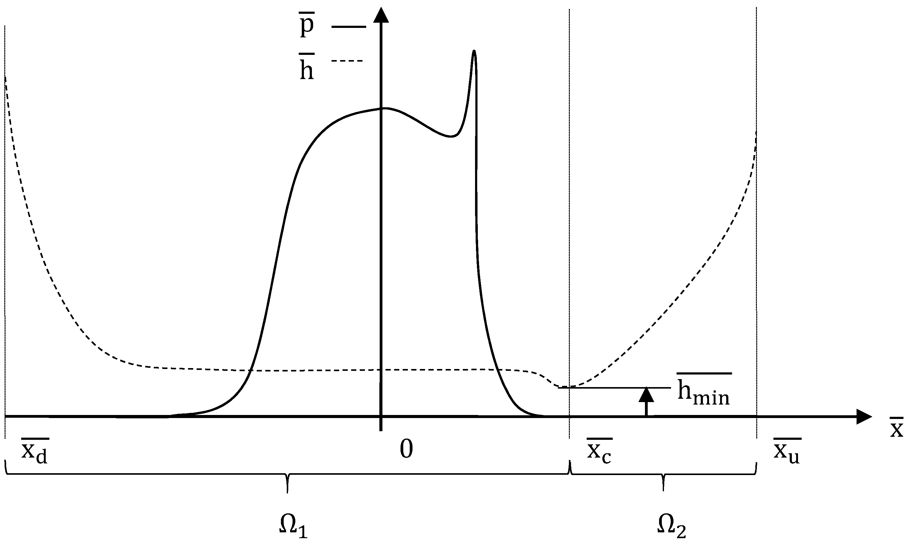
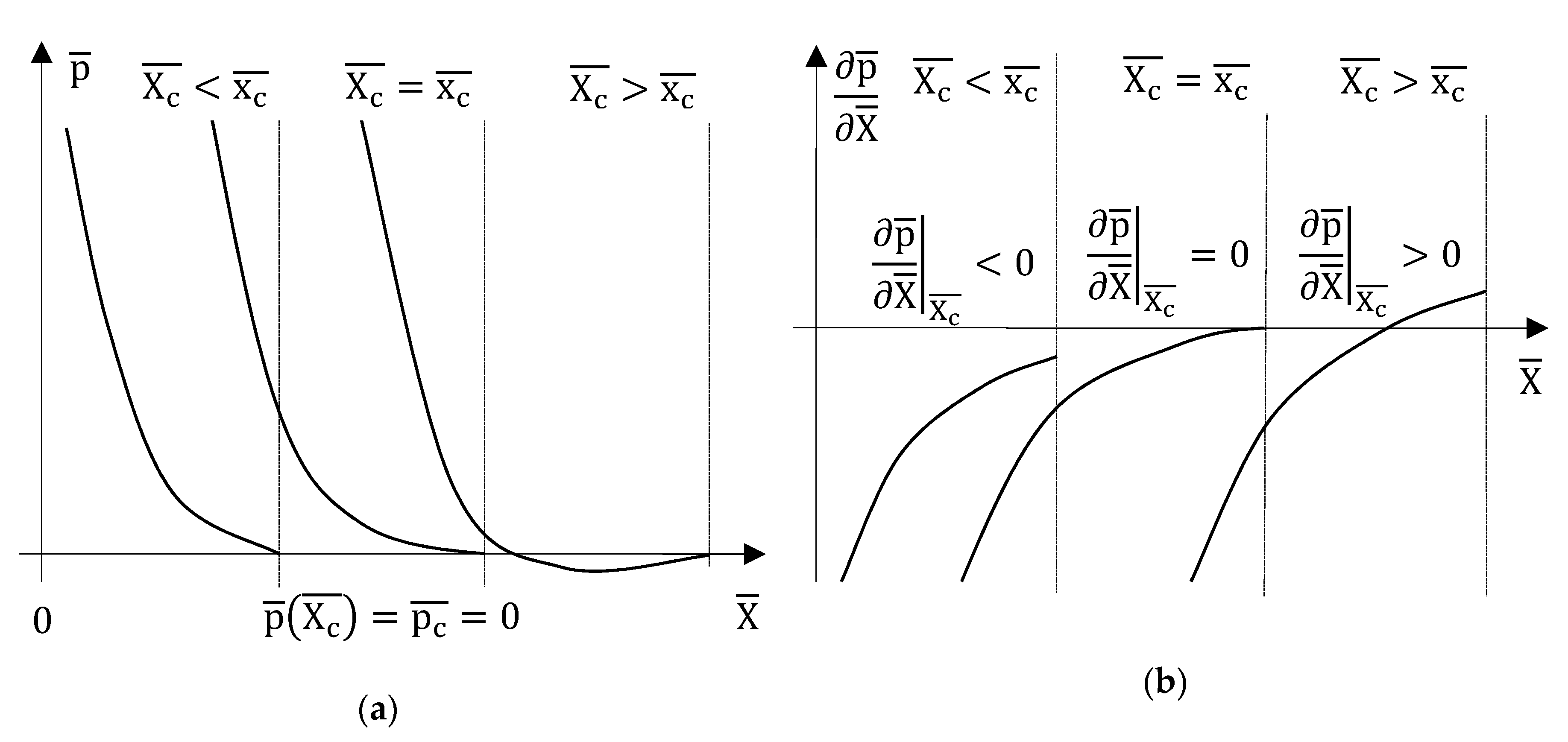
2.3. Investigation of the Minimum Film Thickness

Based on steady-state EHL solutions many authors have derived curve fit equations for the minimum film thickness $\overline{{\mathrm{h}}_{\min }}$ in line contacts and from which we aim to evaluate the results generated by the ALE formulation. Dowson and Higginson [9] were the first to obtain such an expression, this was based on the forward iterative method and considered an incompressible and linear piezoviscous lubricant. This curve fit was developed by Hamrock and Jacobson [50] and Pan and Hamrock [51] who included more representative lubricant behaviour such as the effect of compressibility and Roeland’s viscosity. Later Lubrecht et al. [52] derived a solution based on the multilevel methods and Moe’s non-dimensional parameters. This was further developed by Venner [10] who derived an expression that is considered the best approximation for calculating the minimum film thickness in a line contact to date. It is of note that, despite the differences in model assumptions, the solutions obtained by Dowson and Higginson [9] are widely used because of the accuracy of the solution when comparing to the modern alternatives [53]. All minimum film thickness equations and the corresponding non-dimensional methods can be found in Appendix B.

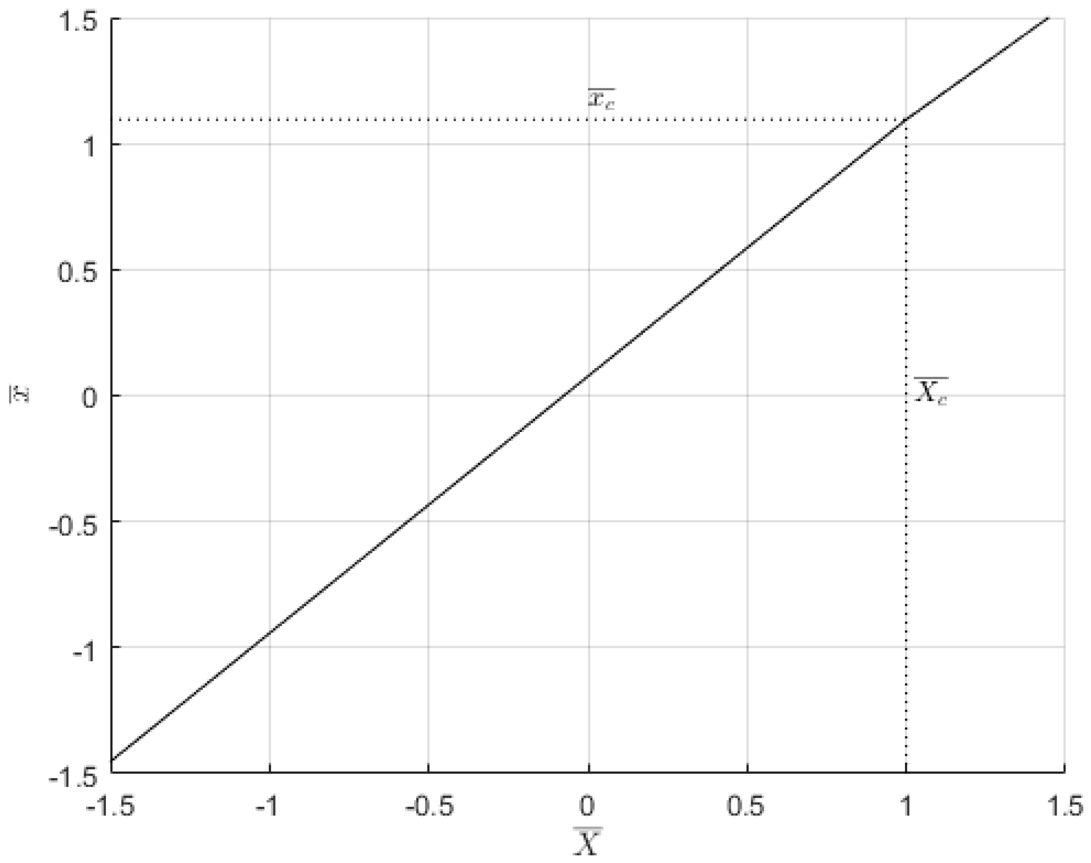
2.4. Comparison of the ALE Formulation with the Heaviside Approach

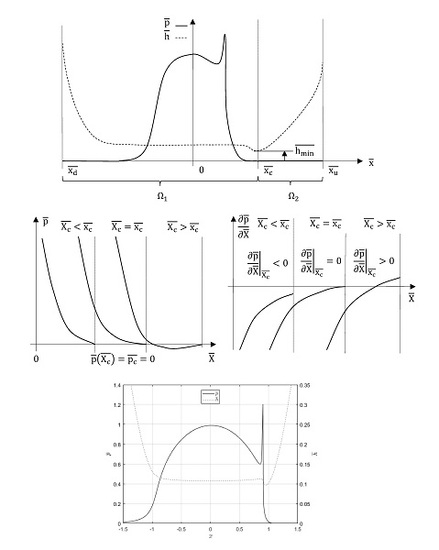
Results of the Elrod model [14] were used to compare with results produced by the ALE formulation in order to analyse the effectiveness and efficiency of the new method. This was conducted under steady-state conditions for which the lubricant was considered isoviscous and linearly compressible. For this purpose the model operating parameters were maintained from Table 1 (at ambient conditions where applicable), with the lubricant bulk modulus specified as $\mathsf{\beta }=500$ MPa and cavitation pressure set to zero gauge. The separation was maintained at $\overline{{\mathrm{h}}_0}=1$ and the conditions for load balance were not applied, corresponding to this the initial pressure distribution was set to zero in the contact. These simplifications allowed the models to be compared under the same operating conditions and computational resources. The Heaviside approach to cavitation can readily be programmed in COMSOL Multiphysics with the derivation and corresponding equations given in Elrod [14]. Within the software the same mesh generation and solution procedure as for the ALE formulation were employed to produce solutions.

3. Results

Results are presented and discussed in this section, demonstrating example solutions obtained using the ALE formulation for cavitation boundary conditions in EHL. The data presented in this section was obtained by using the computer software Matlab [54] to initialise and control the simulations as described in Section 2.2.

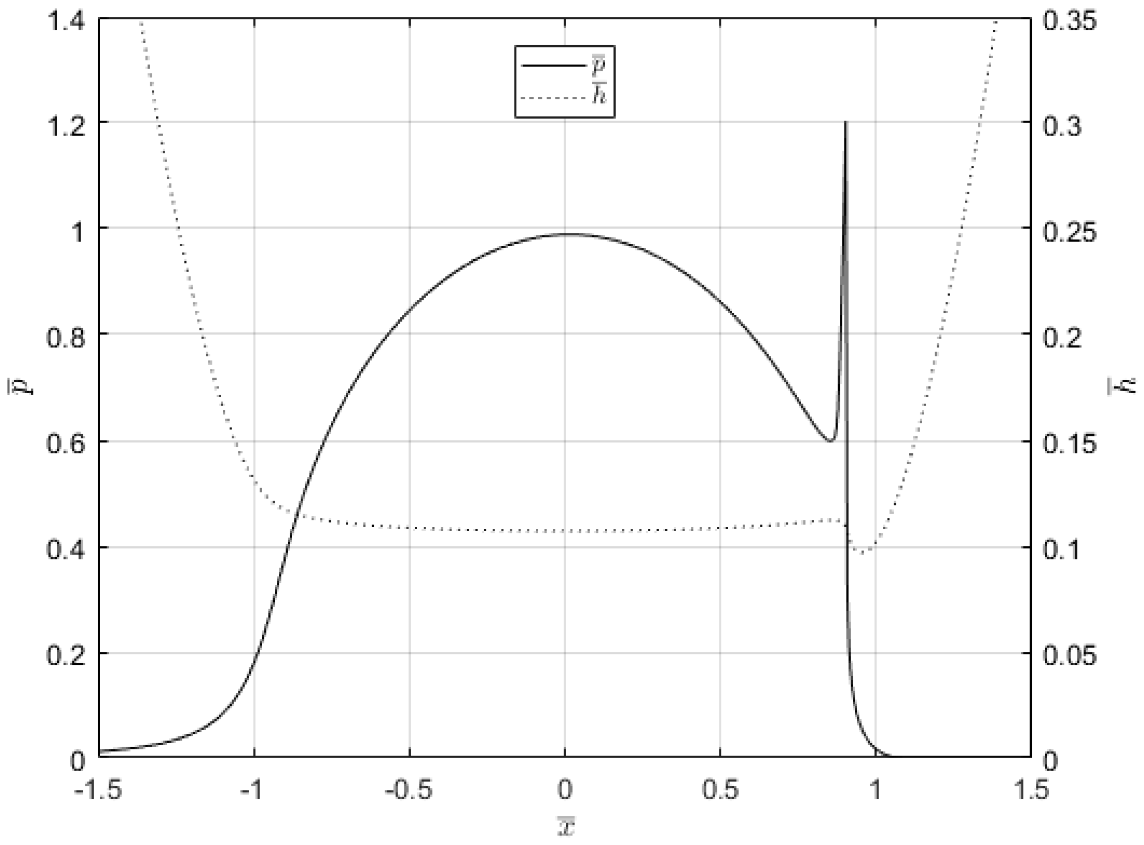
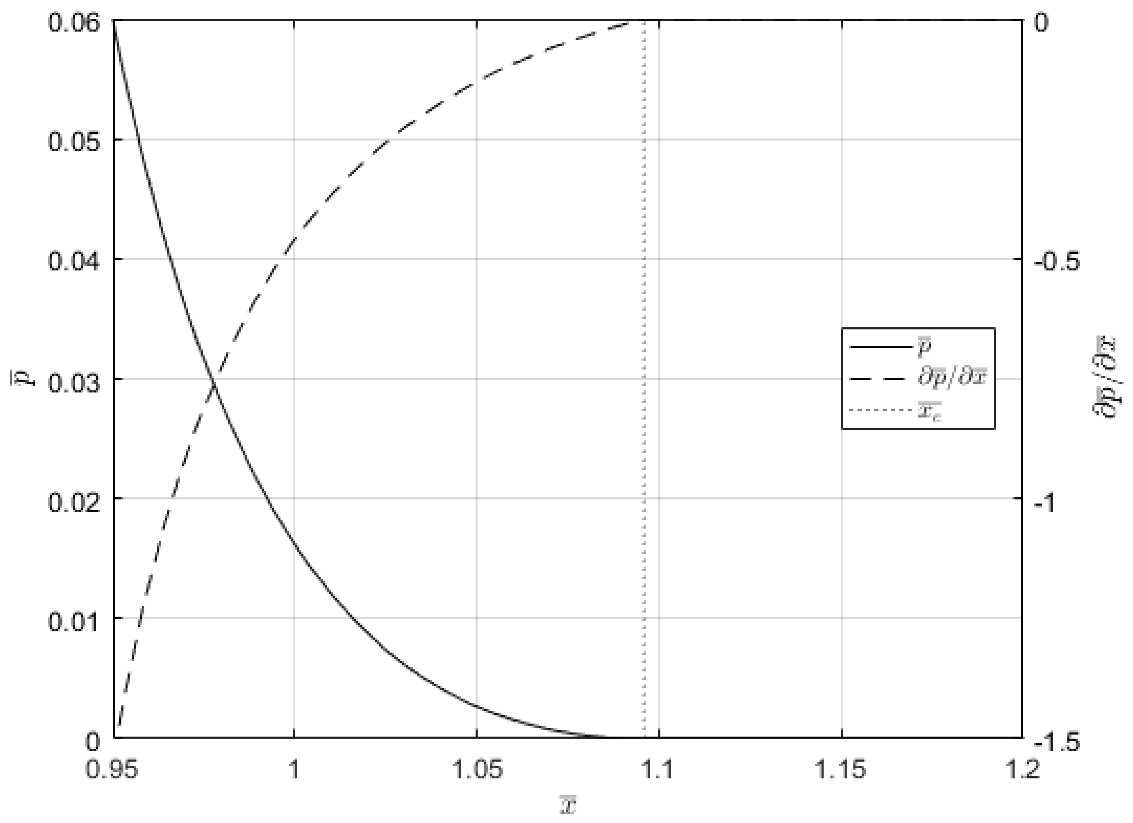
3.1. Steady-State Simulations

Pressure and film thickness distributions for the steady-state EHL solution are shown in Figure 3, both are shown in the spatial frame of reference which was also calculated as part of the solution procedure. The pressure increased from zero downstream up to the Hertz pressure $\overline{\mathrm{p}}=1$ in the centre of the contact, subsequently it reduced then suddenly increased, forming a pressure spike before reducing to zero at the cavitation location from where it remained constant toward upstream. Corresponding to this, the film thickness reduced from downstream toward an almost constant value in the centre of the contact $\overline{\mathrm{h}}=0.101$, then toward the cavitation location a minimum film thickness was reached before it increased towards upstream. These distributions are the expected shape and magnitude of an EHL solution under the conditions imposed and therefore indicates that the ALE formulation is capable of accurately modelling such phenomena.

The solution to the JFO cavitation boundary conditions is given in Figure 4 for the steady-state EHL solution, where both the pressure and pressure gradient tend towards zero at the cavitation location. These are presented in the spatial frame of reference, which moves from the material frame of reference in order to accommodate both the Dirichlet and Neumann constraints imposed for pressure to describe cavitation. The amount by which the cavitation location moves is shown in Figure 5, as is the value of $\overline{{\mathrm{x}}_{\mathrm{c}}}=1.096$ for the problem solved. Figure 5 also demonstrates how the spatial frame is scaled in reference to the material frame to facilitate motion, where the cavitation location moves by the exact amount which reduces the pressure gradient to zero, and the remainder of the domain is moved proportionally such that the upstream and downstream locations are stationary.

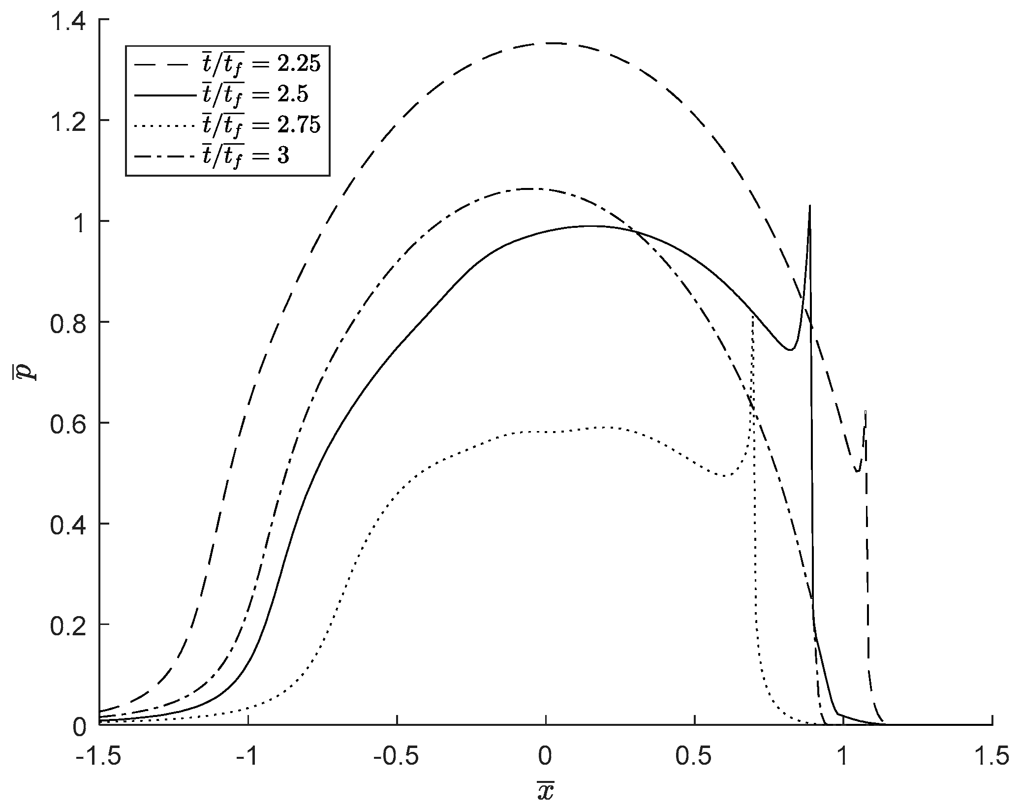
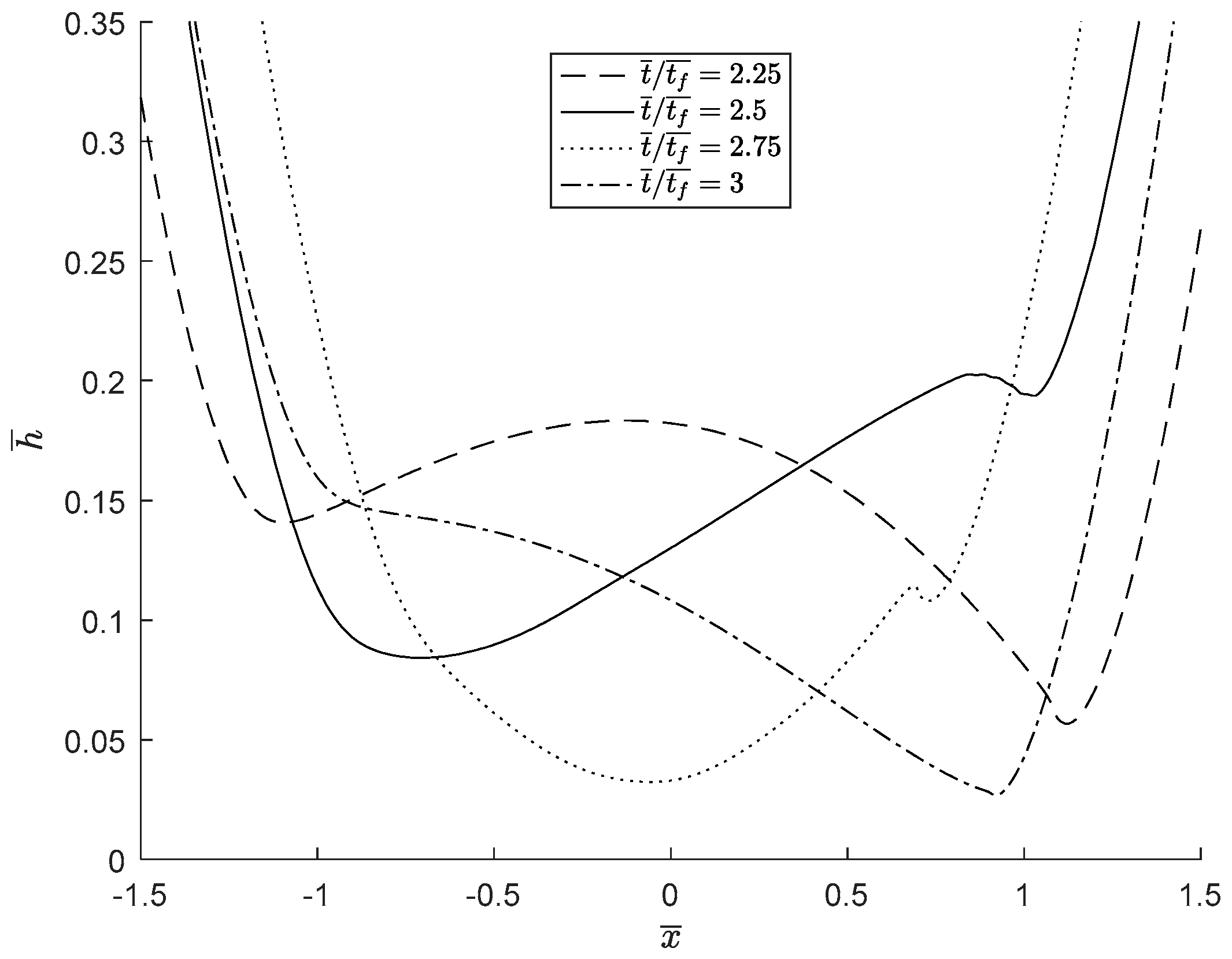
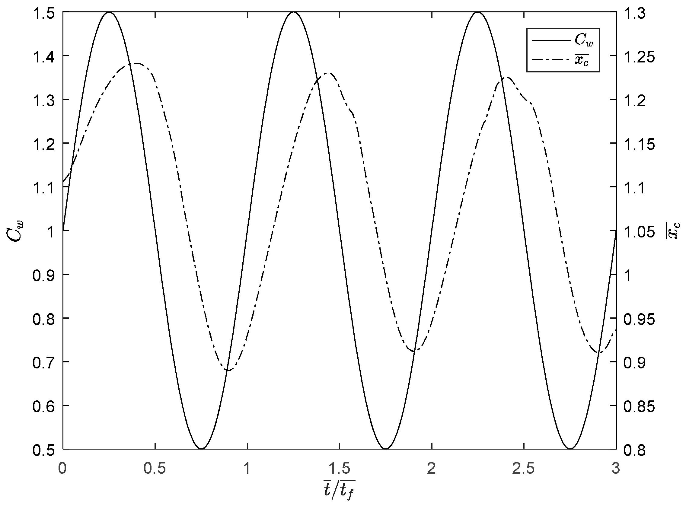
3.2. Transient Simulations

Results generated from the transient simulations showed that the response settled to be periodic with time after the first two complete oscillations. Data obtained over the first three of the five time periods defined in total were therefore been presented. Pressure distributions are given in Figure 6 at time steps $\overline{\mathrm{t}}/\overline{{\mathrm{t}}_{\mathrm{f}}}=2.25,2.5,2.75,3$ for the transient EHL solution, corresponding to this the film thickness distributions are shown in Figure 7. These results indicate the expected response in which an increase in load leads to an increase in pressure and a reduction in film thickness. The pressure in the centre of the contact is increased to 1.33 times and reduced to 0.58 times the initial Hertz pressure when the load is at a maximum and a minimum, respectively. Film thickness is reduced to 0.031 and increased to 0.171 in the centre of the contact at these instances. There are significant differences between the pressure and film thickness distributions given at times $\overline{\mathrm{t}}/\overline{{\mathrm{t}}_{\mathrm{f}}}=2.5,3$ where the load is instantaneously the same. This represents the effect of squeeze in the transient EHL response in which solutions deviate from the steady-state solution and the load-carrying capacity of the contact becomes strongly linked to the rate of change of the film thickness with time.

This deviation of the response over time is further demonstrated in Figure 8 and Figure 9, which show that the loading parameter is exactly periodic with time, whereas the cavitation location, contact separation and minimum film thickness are periodic, but demonstrate anisotropy over a single period. As the load is increased and decreased, the size of the contacting region is also increased and decreased, this causes the cavitation location to move correspondingly as shown by Figure 8. The ALE formulation determines this location with respect to time and implements the required boundary conditions subject to the transient EHL response. Figure 9 shows that the contact separation decreases as the load increases and increases as the load decreases, as was expected. However the minimum film thickness does not follow this trend, instead there are multiple peaks and troughs in the response over a single period. This corresponds to the location of the minimum film thickness being in transition from the near inlet/outlet region to the centre of the contact. This is demonstrated in Figure 7, where at each instance the minimum film thickness is shown to be in motion along the length of the contact.

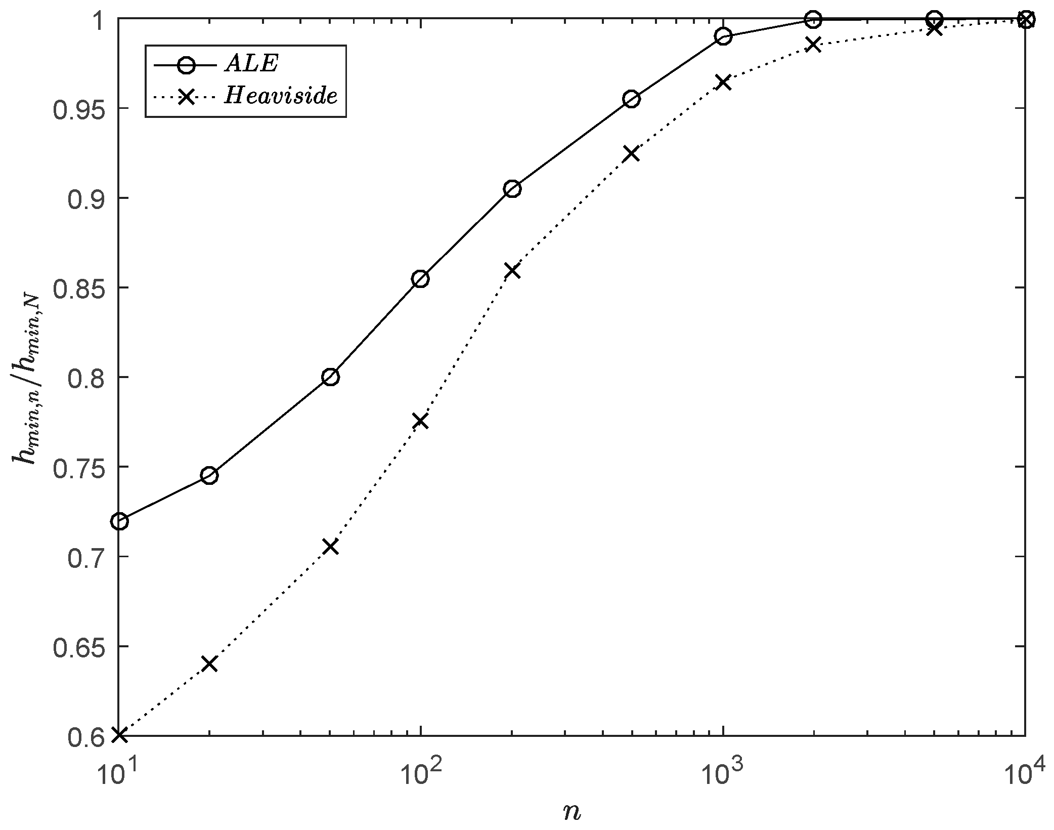
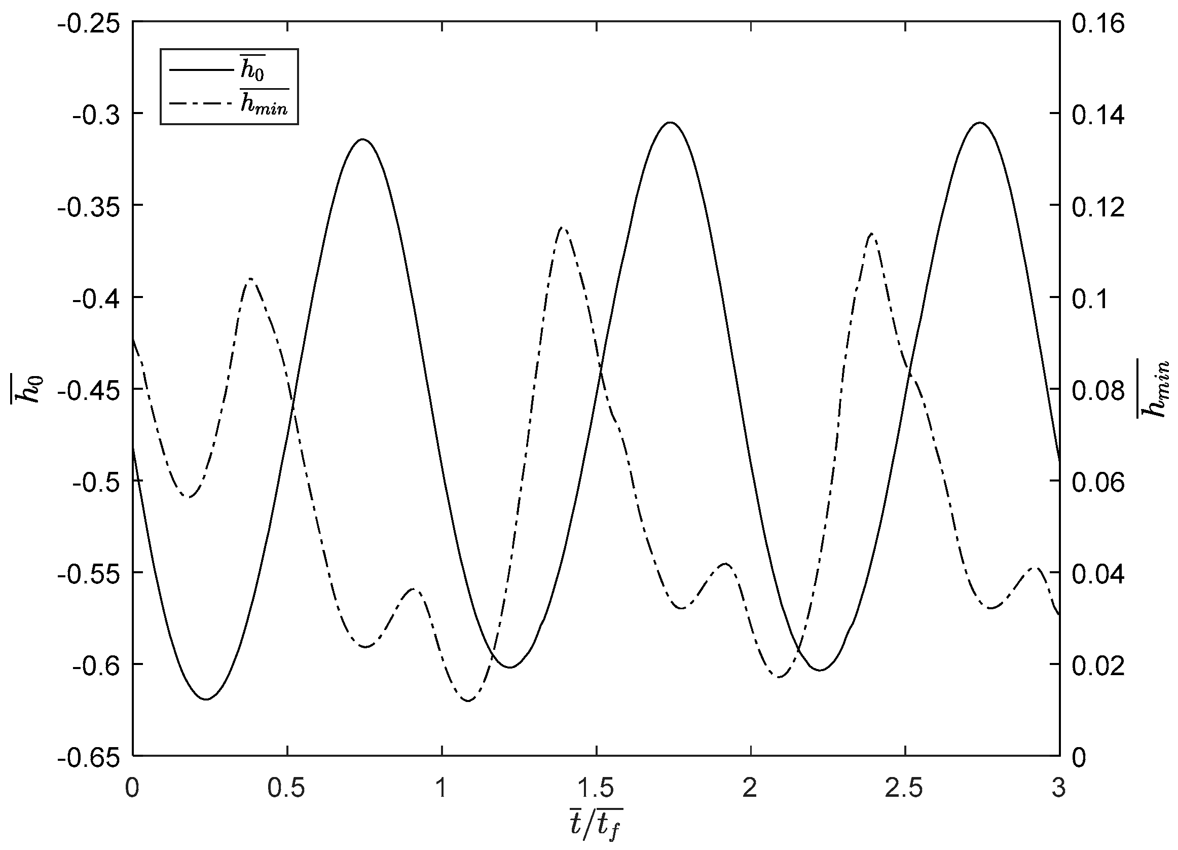
3.3. Analysis of the Minimum Film Thickness

In order to evaluate the ALE formulation, steady-state results were generated over a range of representative operating conditions and compared to equations for the minimum film thickness $\overline{{\mathrm{h}}_{\min }}$ established in the literature. For this purpose the piezoviscous parameters were set to $\mathsf{\alpha }=1.7\times {10}^{-8}$ Pa⁻¹ and $\mathrm{Z}=0.69$ respectively. All other parameters we adjusted accordingly or kept the same as those outlined in Table 1 for the steady-state solution procedure. Subsequently the Moe’s non-dimensional load parameter $\mathrm{M}$ (see Appendix A) was varied over an appropriate range of 10, 20 and 50 for a fixed Moe’s materials parameter $\mathrm{L}=10$. These results were then collated in

Table 3. Minimum film thickness calculations.

Method	$\overline{{\mathbf{h}}_{\mathbf{m}\mathbf{i}\mathbf{n}}}$
	$\mathrm{M}=10,\mathrm{L}=10$	$\mathrm{M}=20,\mathrm{L}=10$	$\mathrm{M}=50,\mathrm{L}=10$
Dowson and Higginson [9]	$1.624\times {10}^{-1}$	$7.443\times {10}^{-2}$	$2.643\times {10}^{-2}$
Hamrock and Jacobson [50]	$1.577\times {10}^{-1}$	$7.325\times {10}^{-2}$	$2.649\times {10}^{-2}$
Pan and Hamrock [51]	$1.519\times {10}^{-1}$	$6.969\times {10}^{-2}$	$2.479\times {10}^{-2}$
Lubrecht et al. [52]	$1.702\times {10}^{-1}$	$7.796\times {10}^{-2}$	$2.768\times {10}^{-2}$
Venner [10]	$1.580\times {10}^{-1}$	$7.338\times {10}^{-2}$	$2.648\times {10}^{-2}$
ALE formulation	$1.576\times {10}^{-1}$	$7.240\times {10}^{-2}$	$2.579\times {10}^{-2}$

for each of the minimum film thickness formulas (see Appendix B) and directly from the ALE method. Note that to account for the different non-dimensionalisation schemes the values were scaled accordingly to match those presented in the rest of the article.

The data presented in Table 3 show that the ALE formulation accurately describes the minimum film thickness $\overline{{\mathrm{h}}_{\min }}$ when compared to the established literature on the subject. The ALE result was shown to be less than 5% from any of the curve fit equations within the range of parameters considered. The ALE formulation therefore is an accurate method for determining the minimum film thickness and subsequently this validates the pressure distributions and other predictions which can be made from the solutions generated. It should be noted that the ALE formulation is limited by the load parameter $\mathrm{M}$, for high values of which the problem becomes mathematically stiff and the series of equations is much harder to solve computationally. The multilevel method [10,11,12] was developed to study this effect and is the preferred approach for highly-loaded EHL problems. However, the ALE formulation can readily be used within a reasonable range of the non-dimensional parameters to solve EHL problems with a high level of accuracy. This is achieved without the computational expense associated with the numerical modelling of cavitation.

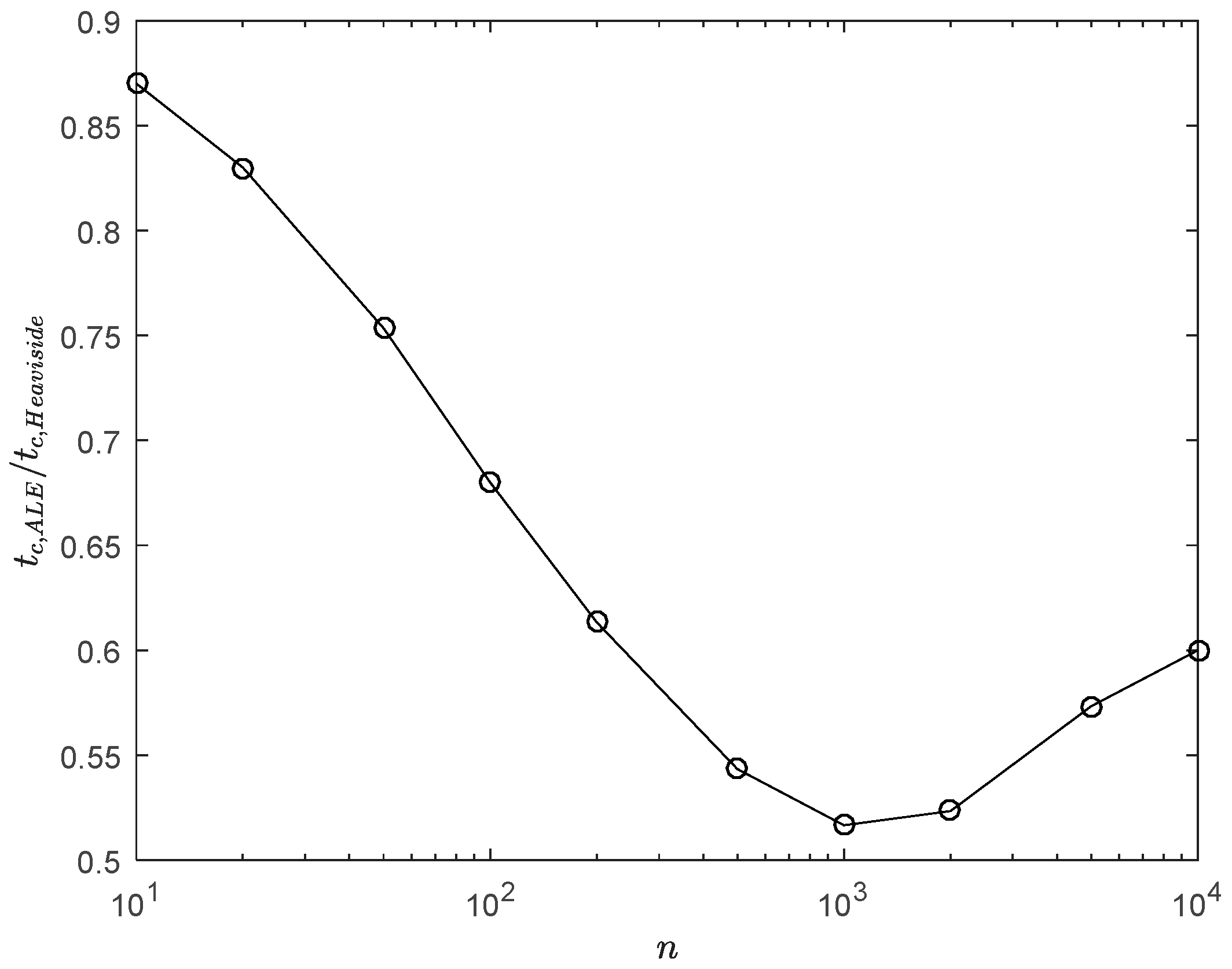
3.4. Analysis of the ALE Formulation and Heaviside Approach

In order to compare the effectiveness of the ALE formulation to that of the Heaviside approach, simulations were undertaken using both methods over a varying number of elements $\mathrm{n}$ up to a maximum $\mathrm{N}$. These simulations were initialised based on the method outlined in Section 2.4. The minimum film thickness reached in each of these simulations was recorded and the ratio of these values determined as a function of the number of elements, where ${\mathrm{h}}_{\min ,\mathrm{n}}$ is the minimum film thickness at any given number of elements and ${\mathrm{h}}_{\min ,\mathrm{N}}$ is the minimum film thickness for the maximum number of elements. Figure 10 presents these trends for both type of approaches, in which it is shown that the convergence of the ALE formulation is better than that of the Heaviside approach. That is where the ratio tends to unity faster for the ALE than compared to the Heaviside, it is also demonstrated that a change of less than 1% is measured at $\mathrm{n}=1000$ for the ALE whereas for the Heaviside $\mathrm{n}=5000$ to achieve the same performance. Additionally, in both cases the resulting values of ${\mathrm{h}}_{\min ,\mathrm{N}}$ were calculated to within 1.34% of each other demonstrating that the results produced by both methods were similar.

Figure 11 presents the ratio of the time to compute using the ALE ${\mathrm{t}}_{\mathrm{c},\mathrm{ALE}}$ to that of the Heaviside approach ${\mathrm{t}}_{\mathrm{c},\mathrm{Heaviside}}$ versus the number of elements used in the simulations $\mathrm{n}$. The value of the ratio is less than unity in call cases considered, which shows that the solutions obtained from the ALE formulation were always calculated faster than the corresponding results based on the Heaviside approach. This clearly demonstrates the efficiency in using the ALE formulation and is the same conclusion as that of Schweizer [42], who noted similar trends when undertaking such a comparison. Interestingly as the number of nodes is increased past $\mathrm{n}=1000$ the efficiency of the ALE formulation begins to diminish comparatively to that of the Heaviside approach. The ALE method has many more degrees of freedom than the same problem defined using Elrod’s model and therefore scales less well as the number of elements increases. For reference at $\mathrm{n}=1000$: ${\mathrm{t}}_{\mathrm{c},\mathrm{ALE}}=13.7$ s and ${\mathrm{t}}_{\mathrm{c},\mathrm{Heaviside}}=26.3$ s; at $\mathrm{n}=10,000$: ${\mathrm{t}}_{\mathrm{c},\mathrm{ALE}}=156.1$ s and ${\mathrm{t}}_{\mathrm{c},\mathrm{Heaviside}}=260.2$ s.

4. Discussion

In this article a new alternative method for modelling cavitation in EHL is presented. This derives an ALE formulation to solve the EHL governing equations in a material frame of reference, which was subsequently moved to a spatial frame of reference where the solution was required. This allowed the JFO cavitation boundary conditions to be implemented such that the cavitation location formed the boundary between the liquid and vapour phases. This location moved proportionately with the error in the Neumann constraint for pressure when determined in the material frame of reference and the Dirichlet constraint was imposed for the liquid phase. The spatial coordinates were additionally solved for, along with those governing fluid flow and load capacity.

Numerical methods were developed and results presented under both steady-state and transient operating conditions, with the distributions of pressure and film thickness exhibiting the shape and magnitude expected from such analyses. For the steady-state simulations, the implementation of the cavitation boundary condition was explored in more detail, and demonstrated how the material coordinates was moved to the spatial coordinates in order to solve for the onset of cavitation. Transient simulations showed how cavitation was modelled with respect to time. Results indicated the effect of squeeze in the response in which there was some deviation from exact periodicity in the cavitation location, contact separation and minimum film thickness under the dynamic loading imposed. Minimum film thickness calculations demonstrated that the ALE formulation accurately describes the EHL response established in the literature [9,10,50,51,52] to within 5% of the predicted values. It was also presented under hydrodynamic conditions that the ALE formulation has better numerical converge and computes in less time than comparative problems solved using the Elrod (Heaviside) approach.

The approach as presented is applicable to lubricants with arbitrary pressure–density and pressure–viscosity relationships; it is a future requirement to include the effect of shear-thinning (non-Newtonian) fluids by reformulating the ALE in application to the generalised Reynolds equation which is used to accurately describe these types of fluid flows. The ALE formulation will also be used to examine problems with a third dimension such as point contacts, which has been investigated by Schweizer [42] under hydrodynamic conditions. The EHL governing equations will be adapted accordingly and the cavitation location will become a cavitation front representing the transition between phases over the contact area. Experimental validation of results generated using the ALE formulation will then be readily achievable and comparisons can be made under matched operating conditions to those considering three-dimensional transient EHL problems in the literature.

Other cavitation-related phenomena such as film reformation, sub-ambient pressures and lower pressure environments (such as those observed in pad bearings and seals where contact pressures are of the order ~10 MPa) will also be formulated into problems which can be solved using an ALE approach. This fundamental work will subsequently allow more complex and irregular geometries to be explored where multiple cavitation locations may be present. Further research will then be needed to explore whether it is a priori that the number of these sites is known, as this is a challenge to modelling cavitation in such problems. The method derived will therefore assist in developing models which describe EHL by including a straightforward means of modelling cavitation.

Results presented were calculated using commercially available software in which the ALE formulation was programmed, this demonstrates that the method can be readily used to solve the difficult numerical problem of EHL using standard practices and commonplace mathematical tools. By removing the complexity of modelling Heaviside or free boundaries, which are usually associated with cavitation [10,14], the equations are less complex to solve and can be calculated without the same numerical requirements. This can be seen as one of the main advantages to using the ALE formulation for EHL, in which solutions to the problem can be obtained to a high degree of accuracy with relative simplicity. Much in the same way that Elrod’s model [14] was established to universally describe cavitation in the fluid and reduce the numerical complexity in modelling the problem.

5. Conclusions

As demonstrated in this article, the ALE formulation for modelling the JFO cavitation boundary conditions in EHL is an effective and straightforward means of implementing such constraints. The approach differs from those currently used for modelling cavitation which either employ a universal equation for describing fluid flow in both the liquid and vapour phases together, or change the solution procedure to ensure a positive pressure. Such approaches rely on Heaviside functions or free boundaries to determine the transition between phases which occurs at the onset of cavitation and as such are subject to additional numerical challenges in addition to those which describe the complex mechanics of EHL. The ALE approach does not require such conditions because the location at which cavitation onset occurs is solved for as part of the solution procedure. The method is a straightforward and accurate means of modelling the JFO conditions in EHL and can therefore been seen as a novel and useful means for the complex issue of numerically solving cavitation problems in lubrication.

References

1. Gohar, R. Elastohydrodynamics, 2nd ed.; Imperial College Press: London, UK, 2002. [Google Scholar]
2. Dowson, D. History of Tribology, 3rd ed.; John Wiley & Sons: Hoboken, NJ, USA, 2009. [Google Scholar]
3. Cameron, A. Basic Lubrication Theory; Longman: London, UK, 1971. [Google Scholar]
4. Floberg, L. Cavitation boundary conditions with regard to the number of streamers and tensile strength of the liquid. In Cavitation and Related Phenomena in Lubrication; IMechE: London, UK, 1974; pp. 31–36. [Google Scholar]
5. Jakobsson, B.; Floberg, L. The Finite Journal Bearing, Considering Vaporization; Gumperts Förlag: Göteborg, Sweden, 1957. [Google Scholar]
6. Olsson, K.-O. Cavitation in Dynamically Loaded Bearings; Scandinavian University Books: Göteborg, Sweden, 1965. [Google Scholar]
7. von Mohrenstein-Ertel, A. Die Berechnung der Hydrodynamischen Schmierung Gekrümmter Oberflächen unter Hoher Belastung und Relativbewegung. In Fortschrittsberichte VDI; Series 1; No. 115. First Published in 1945 in Russian under the name A. M. Ertel; Lang, O.R., Oster, P., Eds.; VDI Verlag: Düsseldorf, Germany, 1949. [Google Scholar]
8. Grubin, A.N. Investigation of the Contact of Machine Components; DSIR Translation No. 337; Central Scientific Research Institute for Technology and Mechanical Engineering: Moscow, Russia, 1949. [Google Scholar]
9. Dowson, D.; Higginson, G.R. Elastohydrodynamic Lubrication; Pergamon Press: Oxford, UK, 1977. [Google Scholar]
10. Venner, C.H. Multilevel Solution of the EHL Line and Point Contact Problems; University of Twente: Enschede, The Netherlands, 1991. [Google Scholar]
11. Venner, C.H.; Lubrecht, A.A. Multi-Level Methods in Lubrication, 1st ed.; Elsevier: Amsterdam, The Netherlands, 2000. [Google Scholar]
12. Habchi, W.; Eyheramendy, D.; Vergne, P.; Morales-Espejel, G.E. Stabilized fully-coupled finite elements for elastohydrodynamic lubrication problems. Adv. Eng. Softw. 2012, 46, 4–18. [Google Scholar] [CrossRef]
13. Wu, S.R. A penalty formulation and numerical approximation of the Reynolds-Hertz problem of elastohydrodynamic lubrication. Int. J. Eng. Sci. 1986, 24, 1001–1013. [Google Scholar] [CrossRef]
14. Elrod, H.G. A cavitation algorithm. J. Tribol. 1981, 103, 350–354. [Google Scholar] [CrossRef]
15. Vijayaraghavan, D.; Keith, T.G., Jr. Development and evaluation of a cavitation algorithm. STLE Tribol. Trans. 1989, 32, 225–233. [Google Scholar] [CrossRef]
16. Bayada, G.; Martin, S.; Vázquez, C. Two-scale homogenization of a hydrodynamic Elrod-Adams model. Asymptot. Anal. 2005, 44, 75–110. [Google Scholar]
17. Bayada, G.; Martin, S.; Vázquez, C. An average flow model of the Reynolds roughness including a mass-flow preserving cavitation model. J. Tribol. 2005, 127, 793–802. [Google Scholar] [CrossRef]
18. Bayada, G.; Martin, S.; Vázquez, C. Micro-roughness effects in (elasto)hydrodynamic lubrication including a mass-flow preserving cavitation model. Tribol. Int. 2006, 39, 1707–1718. [Google Scholar] [CrossRef]
19. Sahlin, F.; Almqvist, A.; Larsson, R.; Glavatskih, S. A cavitation algorithm for arbitrary lubricant compressibility. Tribol. Int. 2007, 40, 1294–1300. [Google Scholar] [CrossRef]
20. Giacopini, M.; Fowell, M.T.; Dini, D.; Strozzi, A. A mass-conserving complementary formulation to study lubricant films in the presence of cavitation. J. Tribol. 2010, 132, 041702. [Google Scholar] [CrossRef]
21. Bertocchi, L.; Dini, D.; Giacopini, M.; Fowell, M.T.; Baldini, A. Fluid film lubrication in the presence of cavitation: A mass-conserving two-dimensional formulation for compressible, piezoviscous and non-Newtonian fluids. Tribol. Int. 2013, 67, 61–71. [Google Scholar] [CrossRef]
22. Fan, T.; Behdinan, K. The evaluation of LCP method in modeling the fluid cavitation for squeeze film damper with off-centered whirling motion. Lubricants 2017, 5, 46. [Google Scholar]
23. Almqvist, A.; Fabricius, J.; Larsson, R.; Wall, P. A new approach for studying cavitation in lubrication. J. Tribol. 2014, 136, 0117061–0117066. [Google Scholar] [CrossRef]
24. Almqvist, A.; Wall, P. Modelling cavitation in (elasto)hydrodynamic lubrication. In Advances in Tribology; Darji, P.H., Ed.; INTECH Open Access Publisher: Rijeka, Croatia, 2016; pp. 197–213. [Google Scholar]
25. Yang, Q.; Keith, T.G., Jr. An elastohydrodynamic cavitation algorithm for piston ring lubrication. STLE Tribol. Trans. 1995, 38, 97–107. [Google Scholar] [CrossRef]
26. Miraskari, M.; Hemmati, F.; Jalali, A.; Alqaradawi, M.Y.; Gadala, M.S. A robust modification to the universal cavitation algorithm in journal bearings. J. Tribol. 2017, 139, 031703. [Google Scholar] [CrossRef]
27. Rothwell, B.; Garvey, S.; Webster, J. A thermal elasto-hydrodynamic lubricated analysis of highly-loaded journal bearings, with varying bulk modulus, to allow high areas of cavitation to be solved. In Proceedings of the 6th World Tribology Congress, Beijing, China, 17–22 September 2017. [Google Scholar]
28. Garcia, G.; Moreno, C.; Vázquez, C. Elrod–Adams cavitation model for a new nonlinear Reynolds equation in piezoviscous hydrodynamic lubrication. Appl. Math. Model. 2017, 44, 374–389. [Google Scholar] [CrossRef]
29. Woloszynski, T.; Podsiadlo, P.; Stachowiak, G.W. Efficient solution to the cavitation problem in hydrodynamic lubrication. Tribol. Lett. 2015, 58, 18. [Google Scholar] [CrossRef]
30. Kumar, A.; Booker, F. A finite element cavitation algorithm. J. Tribol. 1991, 113, 276–284. [Google Scholar] [CrossRef]
31. Grando, F.P.; Priest, M.; Prata, A.T. A two-phase flow approach to cavitation modelling in journal bearings. Tribol. Trans. 2006, 21, 233. [Google Scholar] [CrossRef]
32. Bayada, G.; Chupin, L. Compressible fluid model for hydrodynamic lubrication cavitation. ASME Trans. J. Tribol. 2013, 135, 1–13. [Google Scholar] [CrossRef]
33. Bruyere, V.; Fillot, N.; Morales-Espejel, G.E.; Vergne, P. A two-phase flow approach for the outlet of lubricated line contacts. J. Tribol. 2012, 134, 041503. [Google Scholar] [CrossRef]
34. van Odyck, D.E.A.; Venner, C.H. Compressible Stokes flow in thin films. J. Tribol. 2003, 125, 543–551. [Google Scholar] [CrossRef]
35. van Emden, E.; Venner, C.H.; Morales-Espejel, G.E. Aspects of flow and cavitation around an EHL contact. Tribol. Int. 2016, 95, 435–448. [Google Scholar] [CrossRef]
36. van Emden, E.; Venner, C.H.; Morales-Espejel, G.E. A challenge to cavitation modelling in the outlet flow of an EHL contact. Tribol. Int. 2016, 102, 275–286. [Google Scholar] [CrossRef]
37. Bruyere, V.; Fillot, N.; Morales-Espejel, G.E.; Vergne, P. Computational fluid dynamics and full elasticity model for sliding line thermal elastohydrodynamic contacts. Tribol. Int. 2012, 46, 3–13. [Google Scholar] [CrossRef]
38. Hartinger, M.; Dumont, M.-L.; Ioannides, S.; Gosman, D.; Spikes, H. CFD modelling of a thermal and shear-thinning elastohydrodynamic line contact. J. Tribol. 2008, 130, 041503. [Google Scholar] [CrossRef]
39. Hajishafiee, A.; Kadiric, A.; Ioannides, S.; Dini, D. A coupled finite-volume CFD solver for two-dimensional hydrodynamic lubrication problems with particular application to roller bearings. Tribol. Int. 2017, 109, 258–273. [Google Scholar] [CrossRef]
40. Kärrholm, F.P.; Weller, H.; Nordin, N. Modelling injector flow including cavitation effects for diesel applications. In Proceedings of the 5th Joint ASME/JSME Fluids Engineering Conference (FEDSM2007), San Diego, CA, USA, 30 July–2 August 2007. [Google Scholar]
41. Donea, J.; Huerta, A.; Ponthot, J.-P.; Rodríguez-Ferran, A. Arbitrary Lagrangian-Eulerian methods. In Encyclopedia of Computational Mechanics; Stein, E., de Borst, R., Hughes, T.J.R., Eds.; John Wiley & Sons: Hoboken, NJ, USA, 2004; Volume 1, pp. 1–14. [Google Scholar]
42. Schweizer, B. ALE formulation of Reynolds fluid film equation. J. Appl. Math. Mech. 2008, 88, 716–728. [Google Scholar] [CrossRef]
43. Raske, N.; Hewson, R.W.; Kapur, N.; de Boer, G.N. A predictive model for discrete cell gravure roll coating. Phys. Fluids 2017, 29, 062101. [Google Scholar] [CrossRef]
44. Hewson, R.W. Free surface model derived from the analytical solution of Stokes flow in a wedge. J. Fluids Eng. 2009, 131, 041205. [Google Scholar] [CrossRef]
45. Dowson, D.; Higginson, G.R. Elastohydrodynamic Lubrication: The Fundamentals of Roller and Gear Lubrication; Pergamon Press: Oxford, UK, 1966. [Google Scholar]
46. Roelands, C. Correlational Aspects of the Viscosity-Temperature-Pressure Relationship of Lubricating Oils. Ph.D. Thesis, Technical University Delft, Delft, The Netherlands, 27 April 1966. [Google Scholar]
47. Winslow, A. Numerical solution of the quasi-linear Poisson equations in a nonuniform triangle mesh. J. Comput. Phys. 1967, 2, 149–172. [Google Scholar]
48. COMSOL Inc., USA. COMSOL Multiphysics 5.3 [Computer Software]. 2017. Available online: https://www.comsol.com/ (accessed on 21 December 2017).
49. Joppich, W. Multigrid implementation in COMSOL Multiphysics—Comparison of theory and practice. In Proceedings of the COMSOL Conference 2013, Rotterdam, The Netherlands, 23–25 October 2013. [Google Scholar]
50. Hamrock, B.J.; Jacobson, B.O. Elasto-hydrodynamic lubrication of line contacts. ASLE Trans. 1984, 27, 275–287. [Google Scholar] [CrossRef]
51. Pan, P.; Hamrock, B.J. Simple formulas for performance parameters in elastohydrodynamically lubricated line contacts. ASME J. Tribol. 1989, 111, 246–251. [Google Scholar] [CrossRef]
52. Lubrecht, A.A.; Breukink, G.A.C.; Moes, H.; ten Napel, W.E.; Bosma, R. Solving Reynolds equation for EHL line contacts by application of a multigrid method. Tribol. Ser. 1987, 11, 175–182. [Google Scholar]
53. Lubrecht, A.A.; Venner, C.H.; Colin, F. Film thickness calculation in elasto-hydrodynamic lubricated line and elliptical contacts: The Dowson-Higginson, Hamrock contribution. J. Eng. Tribol. 2009, 223, 511–515. [Google Scholar] [CrossRef]
54. The MathsWorks Inc., USA. Matlab vR017a [Computer Software]. 2017. Available online: https://www.mathworks.com/ (accessed on 21 December 2017).
Figure 1. Sketch of an example elastohydrodynamic lubrication (EHL) solution for the pressure and film thickness in a line contact.
Lubricants 06 00013 g001
Figure 2. A sketch showing the effect of the position of the cavitation location when implementing Dirichlet constraints with respect to: (a) the pressure; and (b) the pressure gradient.
Lubricants 06 00013 g002
Figure 3. Pressure and film thickness distributions for the steady-state EHL solution.
Lubricants 06 00013 g003
Figure 4. Distributions of pressure and pressure gradient showing the implementation of the cavitation boundary condition for the steady-state EHL solution.
Lubricants 06 00013 g004
Figure 5. Material versus spatial coordinates demonstrating motion of the cavitation location for the steady-state EHL solution.
Lubricants 06 00013 g005
Figure 6. Pressure distributions at selected time steps for the transient EHL solution.
Lubricants 06 00013 g006
Figure 7. Film thickness distributions at selected time steps for the transient EHL solution.
Lubricants 06 00013 g007
Figure 8. Dynamic loading coefficient and cavitation location shown as functions of time for the transient EHL solution.
Lubricants 06 00013 g008
Figure 9. Contact separation and minimum film thickness shown as functions of time for the transient EHL solution.
Lubricants 06 00013 g009
Figure 10. Effect of the number of elements on the ratio of minimum film thickness for the arbitrary Lagrangian-Eulerian (ALE) and Heaviside formulations.
Lubricants 06 00013 g010
Figure 11. Effect of the number of elements on the ratio of compute time between the ALE and Heaviside formulations.
Lubricants 06 00013 g011