
Advanced Plasticity Modeling for Ultra-Low-Cycle-Fatigue Simulation of Steel Pipe
by
 ,
,
Rongting Li
1,2,* ,
,
Philip Eyckens
2,
Daxin E
1,*,
Jerzy Gawad
3,
Maarten Van Poucke
4,
Steven Cooreman
4 and
Albert Van Bael
2,* 1
School of Materials Science and Engineering, Beijing Institute of Technology, Beijing 100081, China
2
Department of Materials Engineering, KU Leuven, Kasteelpark Arenberg 44-Box 2450, 3001 Heverlee, Belgium
3
Department of Computer Science, KU Leuven, Celestijnenlaan 200A, 3001 Leuven, Belgium
4
OnderzoeksCentrum voor de Aanwending van Staal, Technologiepark 935, 9052 Zwijnaarde, Belgium
*
Authors to whom correspondence should be addressed.
Metals 2017, 7(4), 140; https://doi.org/10.3390/met7040140
Submission received: 5 March 2017
/
Revised: 11 April 2017
/
Accepted: 13 April 2017
/
Published: 14 April 2017
(This article belongs to the Special Issue Advances in Plastic Forming of Metals)
Abstract
:Pipelines and piping components may be exposed to extreme loading conditions, for instance earthquakes and hurricanes. In such conditions, they undergo severe plastic strains, which may locally reach the fracture limits due to either monotonic loading or ultra-low cycle fatigue (ULCF). Aiming to investigate the failure process and strain evolution of pipes enduring ULCF, a lab-scale ULCF test on an X65 steel pipeline component is simulated with finite element models, and experimental data are used to validate various material modeling assumptions. The paper focuses on plastic material modeling and compares different models for plastic anisotropy in combination with various hardening models, including isotropic, linear kinematic and combined hardening models. Both isotropic and anisotropic assumptions for plastic yielding are considered. As pipes pose difficulty for the measurement of plastic properties in mechanical testing, we calibrate an anisotropic yield locus using advanced multi-scale simulation based on texture measurements. Moreover, the importance of the anisotropy gradient across thickness is studied in detail for this thick-walled pipeline steel. It is found that the usage of a combined hardening model is essential to accurately predict the number of the cycles until failure, as well as the strain evolution during the fatigue test. The advanced hardening modeling featuring kinematic hardening has a substantially higher impact on result accuracy compared to the yield locus assumption for the studied ULCF test. Cyclic tension-compression testing is conducted to calibrate the kinematic hardening models. Additionally, plastic anisotropy and its gradient across the thickness play a notable, yet secondary role. Based on this research, it is advised to focus on improvements in strain hardening characteristics in future developments of pipeline steel with enhanced earthquake resistance.
1. Introduction
The finite element (FE) method has been widely used in the design and implementation of metal forming to predict the distribution of stress and strain in the formed part. Metal forming is usually a complex process in which material properties, i.e., microstructure, crystal orientation, flow stress and plastic anisotropy, will change due to the accumulation of the local plastic deformation. In general, the constitutive plasticity modelling significantly influences the attainable accuracy in FE simulations. As discussed next, the constitutive model is composed of two aspects, i.e., a hardening model and a yield locus model.
Isotropic hardening is often assumed in numerical simulations of sheet metal forming processes. It has the advantage of simplicity, but only approximates real material behavior, as for instance, it is unable to present the Bauschinger effect, which is encountered in many metals. The Bauschinger effect is characterized by a reduced yield stress upon load reversal after initial plastic loading. For instance, in uniaxial tension followed by compression, the flow stress in compression is significantly lower than the flow stress at the end of tensile prestraining. To enable modeling of the Bauschinger effect, the linear kinematic hardening rule has been proposed [1], which translates the yield locus by the kinematic stress tensor or back stress tensor with a single constant hardening modulus. Combined hardening models have also been introduced, which integrate isotropic and kinematic hardening, e.g., as illustrated in Wu [2] and Chung et al. [3]. Combined hardening models may reproduce the Bauschinger effect more accurately, at the cost of a more elaborate hardening parameter identification procedure.
The earliest yield locus for anisotropic plastic deformation was derived by Hill [4] as a straightforward extension of the isotropic von Mises yield locus [5]. The anisotropy parameters of the classical Hill’48 yield locus are usually identified from Lankford coefficients (r-values) measured in tensile test in three directions. More recent yield criteria require more effort in terms of the experimental calibration. Barlat’s criterion Yld2000-2D [6] requires eight measurements: three directional yield stresses obtained from the uniaxial tensile tests, σ0, σ45, σ90, and corresponding r-value, r0, r45 and r90. Additionally, it requires the equibiaxial yield stress σb and the equibiaxial r-value rb, which are typically obtained from either disk compression or bulge test. To provide more accurate predictions, yield locus expressions with more coefficients have been introduced, which necessitate more material tests for calibration. For example, the Yld2004-18p [7] yield function includes 18 parameters; the criterion BBC2008 [8] needs 16 or 24 parameters; and the CPB06 [9] yield locus may contain 28 anisotropy coefficients.
As mentioned above, the coefficients in these yield criteria are typically identified based on the results of various mechanical tests that probe particular points on the yield locus. This entails much technical complexity and methodological issues in ensuring consistency among the tests, which in turn increase the cost of experiments needed for calibration of anisotropy coefficients. To circumvent this issue, one may employ virtual experiments that either replace or complement mechanical testing [6]. The virtual experiments often use multilevel polycrystal plasticity models that derive macroscopic plastic behavior from microstructural features via a homogenization procedure applied on the material response at the micro-scale level. Embedding crystal plasticity models directly in large-scale FE simulations is computationally extremely demanding. Therefore, Van Houtte et al. [10] have established the facet method using homogeneous polynomials to describe the plastic potential in either stress or strain rate space, which comprises much more coefficients than the conventional phenomenological constitutive law. These coefficients have been readily derived from a series of virtual experiments performed on the basis of, e.g., the Taylor or the ALAMEL (Advanced Lamel model) models [11,12,13,14,15,16].
Ultra-low cycle fatigue (ULCF) testing typically applies cyclic loads that induce a small amount (a few percent) of plastic deformation, which leads to failure after applying a low number of cycles, usually less than a hundred. Kanvinde and Deierlein [17] consider that ULCF is in the range of 10–20 cycles, and Xue [18] put the limit to 100 for ULCF. Despite these differences, there is a general agreement that the failure is driven by the plastic response of the material attributed to ULCF [19]. However, the characterization of the parameters driving ULCF was not found until numerous experimental research works were carried out to calibrate the material constants for various metals in the 1950s. The classical constitutive model of predicting material failure due to ULCF is the Barcelona plastic damage model initially proposed by Lubliner et al. [20], which is based on an internal variable-formulation of plasticity theory for the non-linear analysis of concrete. Martinez and Oller et al. [21] developed a new plastic-damage formulation to simulate the mechanical response and failure due to ULCF specially for steels. It is based on the Barcelona plastic model, but provides enhancements by adding a non-linear kinematic hardening law coupled with a new isotropic hardening law. Van Poucke et al. [22] performed simulations of a large-scale bending test under cyclic loading and validated it with experimental ULCF on pipes with or without defect. Different hardening models are considered (isotropic hardening, non-linear kinematic hardening and combined hardening) in combination with isotropic yield locus (von Mises). Assuming combined hardening, the buckle may be accurately predicted for the ULCF test with a buckle-initiating defect. Without such a defect, however, failure occurs near clamping in the test, which could not be accurately predicted, attributed to insufficient modelling of the clamping conditions.
As each combination of the homogenization response of polycrystalline plasticity models and hardening models will lead to a yield criterion [14], the aim of the paper is to investigate the capability of advanced plastic anisotropic yield criteria to represent the behavior of steel pipe during the ULCF forming process including the material failure and the strain evolution, on the basis of the study of Van Poucke et al. and Van Wittenberghe [22]. The advanced plastic anisotropic yield criteria adopted in this research are:
- (1)
- isotropic hardening model combined with von Mises, Hill and facet yield loci.
- (2)
- linear kinematic hardening model in combination with von Mises and Hill yield loci.
- (3)
- combined hardening model combined with von Mises and Hill yield loci.
The adopted anisotropic yield loci (Hill and facet) are calibrated by the ALAMEL polycrystal plasticity model. To investigate the accuracy of the above yield criteria on the prediction of cycles before ULCF failure and strain evolution during the process, finite element simulations were carried out using ABAQUS (6.13, DS SIMULIA, Paris, France) and validations were made with large-scale ULCF experimental results.
2. ULCF Testing and FE Simulation Setup
2.1. Experimental Test Setup
In the full-scale ULCF test of straight pipe (Figure 1), the pure-bending method was selected. The tube is welded to both tube holders to prevent any relative rotation and translation during the test. The test input was a cylinder displacement, and the bending moment in the bending setup was delivered by hydraulic cylinders with a capacity of 500 kN on a moment arm of 2 m, giving the setup a bending capacity of 1000 kNm [22]. The test sample was filled with water and slightly pressurized (to 0.27 MPa). During the test, the water pressure value was monitored to serve as a leak detection where a sudden pressure drop indicates a through-thickness crack. The tube holder was fixed to the tube by using a small weld to avoid a rotational and longitudinal movement of the tube inside the tube holder.
2.2. Finite Element Simulation Setup
The simulations of a four-point bending test were used to validate the experimental ultra-low cycle fatigue (ULCF) tests on pipes as shown in Figure 2. In the Finite Element (FE) simulation, the pipe displacement was imposed in two points along the pipe length (Reference Points (RP) 3 and 4 in Figure 2) with the cyclic loading schedule in the X-direction as shown in Figure 3. In the simulations, the hydraulic cylinder displacement was calculated out of RP 5, 6, 7 and 8 displacements. A single cycle comprises bending in one way followed by unloading, then bending in the other way and finally unloading.
A kinematic coupling interaction was defined in Reference Points 3 and 4 to generate a rigid connection of the reference point with the pipe surface, similarly as the welded connections between the tube and tube holders in the experiment. One support joint (RP1) was axially restrained, and another support (RP2) was only allowed to move freely in the tube axial direction. Like in the experimental test, an internal pressure was imposed on the inner surface of the tube in the simulations, and an axial force in RP2 was defined as the result of pressure on the pipe end section.
Shell elements with four nodes and reduced integration (S4R) were selected for the deformable tube. Having an element size of approximately 10 mm by 12 mm, it resulted in 20,104 elements in total for the tube mesh.
3. Material Model Description
3.1. Pipe Material
The large-scale ULCF tests were performed using an on-shore pipeline of X65 steel. Geometric parameters describing the considered tube are illustrated in Figure 4. To initiate buckling at the pipe center, 1 mm of thickness was removed in a central zone of 200 mm length and 60 mm width at either side (0° and 180° around circumference). The initial steel sheet was formed from a hot-rolled coil by uncoiling and levelling in a cold forming process. Next, the tube was rolled by a series of non-cylindrical rolls and high frequency welded along the axial direction.
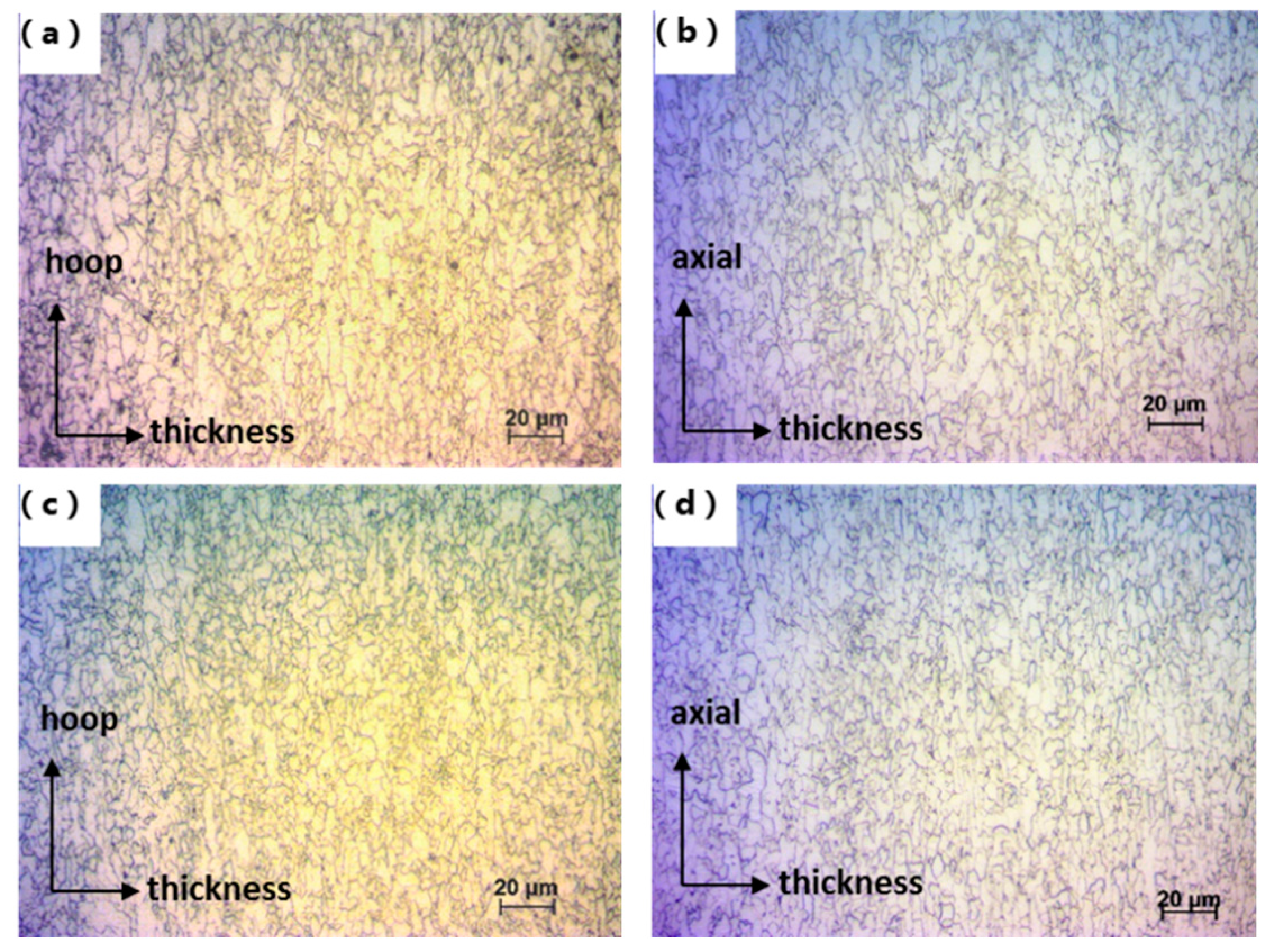
The optical microstructure analysis of the tube was performed in multiple sections. As shown in Figure 5, the microstructure is composed of ferritic (bcc) grains with a small fraction of bainite along ferritic grain boundaries. The average grain diameter is about 5 μm.
3.2. Plastic Strain Hardening
3.2.1. Mechanical Tests
To test the material properties under different stress and strain paths, monotonic tensile tests and a cyclic tension-compression test were performed.
In the monotonic tensile tests, full-thickness tensile specimens of dog-bone geometry, oriented along tube axial direction, have been tested (without prior flattening of the sample). Three tests were performed to guarantee repeatability. The obtained stress-strain curve is presented in Figure 6 for the X65 steel pipe for the monotonic tensile test. The average yield stress and ultimate tensile strength are respectively about 595 MPa and 692 MPa.
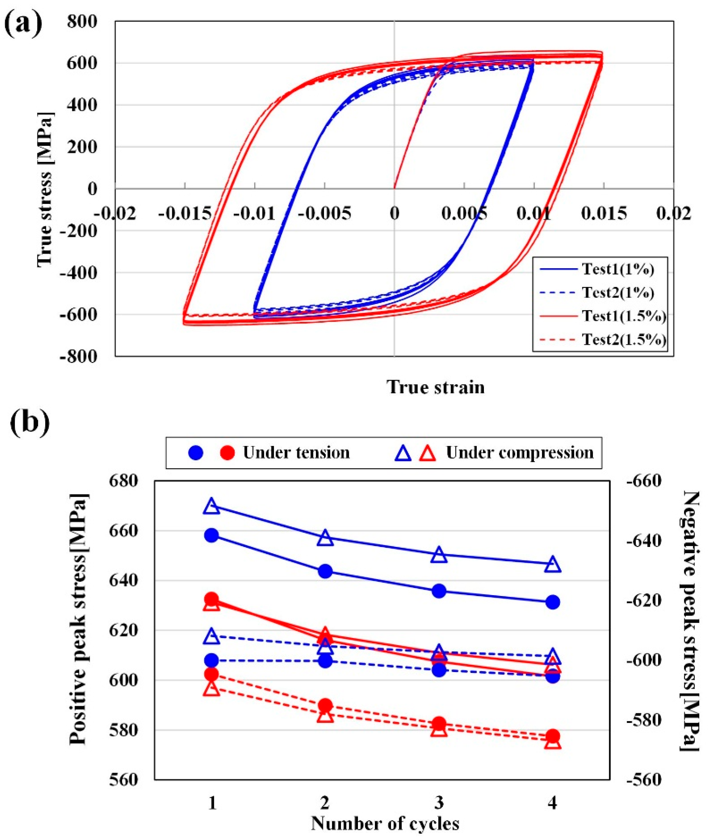
In cyclic tension-compression tests, flat samples of a 3-mm thickness were extracted with face mill and subsequently polished to avoid premature failure. Samples were oriented along the tube axial direction. The tests were performed with strain amplitudes of 1% and 1.5% (Figure 7a). It was observed in Figure 7b that the stress value decreased gradually as the number of cycles increased under all conditions.
3.2.2. Strain Hardening Models
The differences between the isotropic, kinematic and combined hardening models lies in the relationship between yield function and flow stress, as described by continuum mechanics. Neglecting temperature dependence and assuming rate-insensitive behavior, the following general yield criterion holds:
where the yield function is a positive, homogeneous function of one degree, is the stress tensor, is the back stress tensor and represents the flow stress (yield stress), which is a function of the equivalent plastic strain .
- (1)
- For the isotropic hardening, the Voce hardening law is used:which defines the evolution of the flow stress , as a function of the equivalent plastic strain . Here, is the yield stress; is the change of yield surface size at saturation; and b is the rate at which the yield surface grows as plastic straining develops. The stress-strain is calibrated from the quasi-static tension tests presented in Figure 6. For isotropic hardening, the back stress .
- (2)
- For the linear kinematic hardening, the evolution law (3) describes the translation of the yield surface in stress space through the backstress with constant hardening modulus :
The flow stress is a piece-wise linear function of equivalent strain; cf. Table 1. All parameters are calibrated by fitting to uniaxial tensile and tension-compression data.
- (3)
- The evolution law of combined hardening model consists of two components: (i) a nonlinear kinematic hardening component as:in which the kinematic hardening modulus and kinematic hardening exponent are calibrated from cyclic test data and (ii) an isotropic hardening component Equation (2).
Material parameters are given in Table 1 for different hardening models.
3.3. Plastic Anisotropy
3.3.1. Texture Measurements
The non-random orientation of crystal lattice planes, or (crystallographic) texture, is the main microstructural data to calibrate the ALAMEL multi-scale model [23]. The texture at different locations along the tube hoop direction and across the tube wall thickness direction have been measured by X-ray diffraction experiments, from which orientation distribution functions (ODFs) were calculated. A discrete set of 5000 orientations, representative for the texture, was extracted from the continuous ODFs using the STAT algorithm in the MTM-FHM software [24].
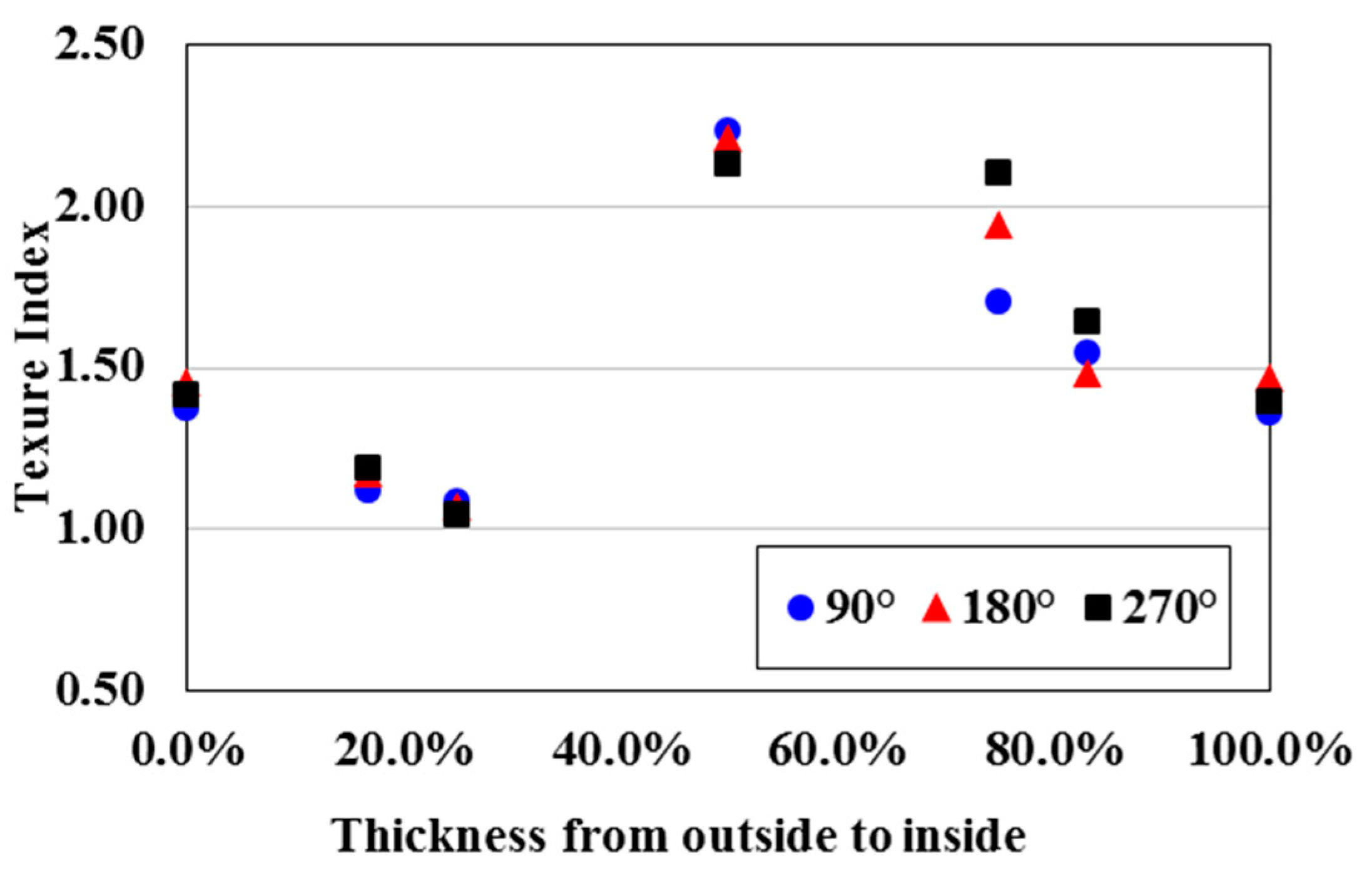
Figure 8 shows 2 = 45° sections of the ODFs of the measured texture for the investigated steel tubes at seven different depths (from outer to inner tube surface: 0%/16.7%/25%/50%/75%/83.3%/100%) and three locations (90°/180°/270°) along the tube hoop direction. A significant texture gradient across thickness is observed. The texture intensity or texture sharpness is quantitatively represented by the texture index (TI) integrated by the square of the ODF function over the entire Euler space:
It is shown in Figure 9 that the texture at 50% depth across thickness has the sharpest texture (highest TI) and that the texture at 25% depth possesses the lowest TI value, which is close to a random texture (i.e., TI = 1).
Figure 10 shows 2 = 45° sections of the merged texture at equal depths across the thickness of three locations along the hoop direction. Further results are merged in the ODF of the overall merged texture of both hoop and thickness direction, as presented. These merged texture data are used as the input data of the multi-scale virtual experiments for the Hill anisotropy calibration, as detailed next.
3.3.2. Advanced Plasticity Modeling
In this study, the following isotropic and anisotropic yield loci have been employed in the FE simulations in order to check their influence on the prediction of ULCF:
- (1)
- von Mises: the isotropic von Mises yield function calibrated by giving the value of the uniaxial yield stress as a function of uniaxial equivalent plastic strain.
- (2)
- Hill-average: the anisotropic Hill yield function calibrated by r-values in three directions. The r-values are obtained from the ALAMEL multi-scale model on the basis of the overall average texture.
- (3)
- Hill-gradient: the Hill yield function with different r-value parameters for the different integration points across tube thickness. They are calibrated by the ALAMEL model from the corresponding texture gradient.
- (4)
- Facet: the anisotropic facet yield function with 360 parameters, calibrated to closely reproduce the behavior of ALAMEL under all conceivable deformation conditions.
The Hill-average, Hill-gradient and facet criteria are detailed in the next paragraphs.
3.3.3. The Hill-Average Yield Function
The quadratic yield function proposed by Hill [4] is a widely used anisotropic yield function for orthotropic materials. It is given by:
in which the stress tensor is expressed in a coordinate system aligned with the main directions of orthotropic symmetry, in this case being a cylindrical Cartesian coordinate system having its first reference direction aligned with the tube axial direction, second with the hoop direction and third with the radial (tube thickness) direction. If the equation holds, the material is yielding at the considered material point.
It is commonly assumed that the yield point in pure shear is independent of the plane and direction, which means that L = M = N. Defining the flow stress as the uniaxial tensile stress in the uniaxial tensile test along rolled direction (RD), it follows that G + H = 1. Therefore, out of six, there remain three independent Hill parameters, which can be associated with the r-values in uniaxial tensile tests at 0°, 45° and 90° to RD, as follows:
For the simulations with the Hill-average yield function, only one material definition and one shell section are defined for the whole tube part. As pipes pose difficulty for the measurement of plastic properties (r-values) in tensile testing along directions other than the axial direction, the r-values in the Hill-average yield criterion are calibrated based on an advanced identification algorithm: the crystal plasticity virtual experiment framework (VEF) [13,15]. The VEF is a software suite that manages high-level stress-based virtual testing capabilities (e.g., uni- and multi-axial tensile/compressive testing, yield locus and r-value calculation) for multi-scale plasticity models that have been developed for strain-rate-based input of plasticity, such as ALAMEL.
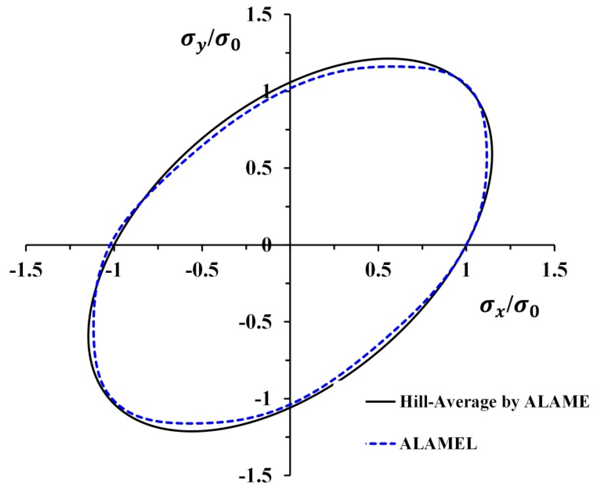
The above overall merged texture (in Section 3.3.1) is used as input data of virtual experiments to calibrate the anisotropy coefficients: r0, r45 and r90 in Table 2. From Equations (7)–(10), the Hill-average normalized – yield locus section is readily generated as shown in Figure 11 (“Hill-average by ALAMEL”). The recalibrated normalized yield locus section by VEF based on ALAMEL is also obtained as shown in Figure 11 (“ALAMEL”). Whereas the quadratic Hill yield criterion generates an elliptic yield locus shape, the yield locus generated directly by ALAMEL deviates from elliptic shape. It can also be seen that the slope of yield locus contours coincide for the point on the horizontal and vertical axes, corresponding to calibration by r0 and r90, respectively.
3.3.4. The Hill-Gradient Yield Function
For the simulations with the Hill-gradient yield locus, Figure 12 illustrates the shell section definition. For the region without thickness reduction (Shell Section 1), five material definitions across thickness are imposed, while for the region with reduced thickness (Shell Section 2), four material definitions are used.
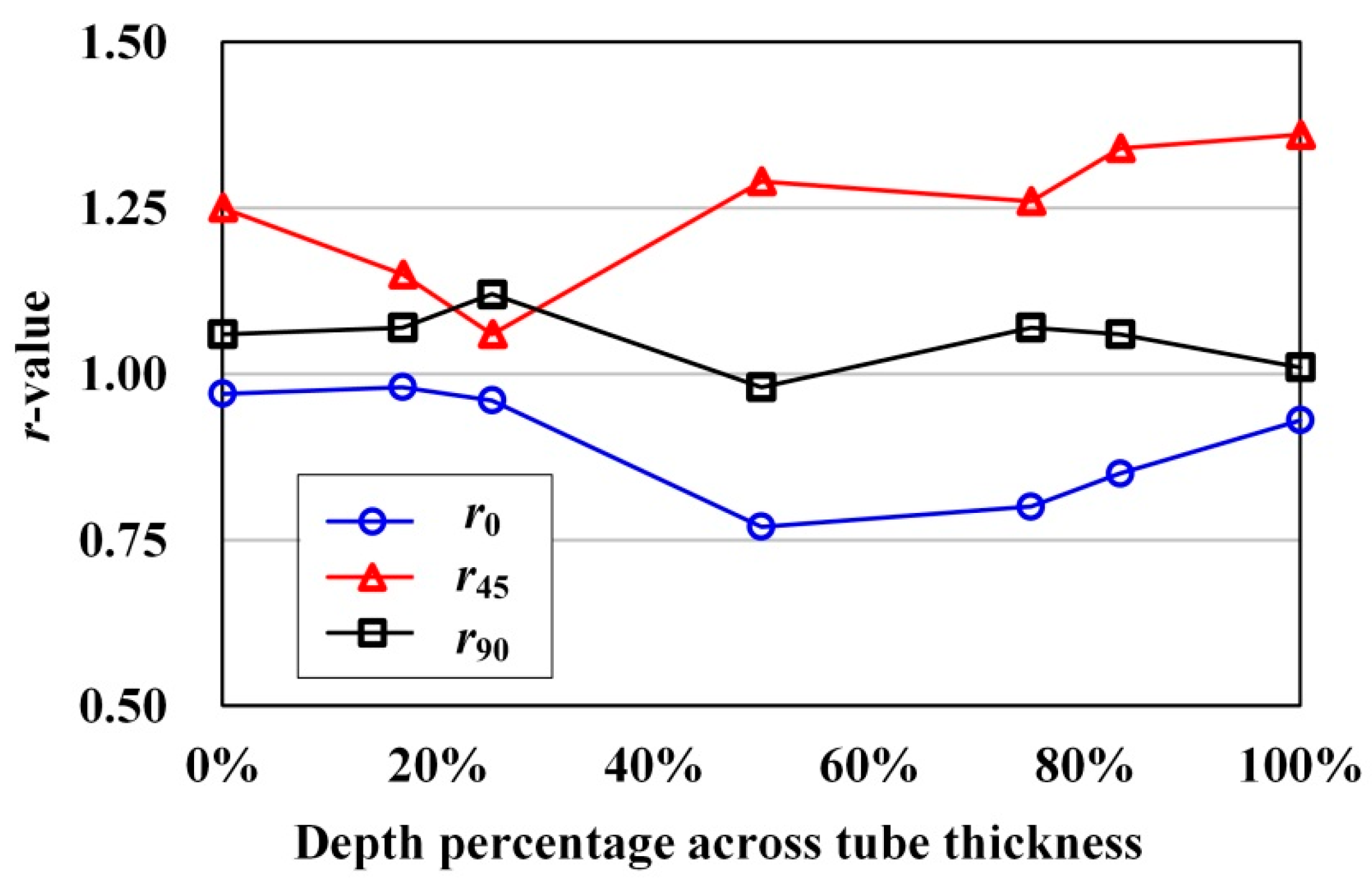
Five sets of r-values corresponding to the merged texture data at five different depths across tube thickness are also calibrated by means of VEF algorithm as shown in Figure 13. Note that at 16% and 25%, the behaviour is near-isotropic (all the r-values close to one), which corresponds to the very weak texture found at these depths. Two-dimensional sections of the yield surfaces, as calculated by ALAMEL, are presented for these for textures at different depths in Figure 14. A significant gradient in plastic properties (r-values and yield surfaces) across thickness is observed.
3.3.5. The Facet Yield Function
Van Houtte et al. [10] have proposed the facet expression, describing the plastic potential by means of a homogeneous polynomial. This mathematical formulation can be used in either strain rate space or stress space. The following is a brief introduction of the method.
Using the description of plastic potential accounting for the plastic anisotropy of textured polycrystalline materials [13], is defined as the plastic potential in strain rate space scaled by the equivalent stress and be expressed as:
where is the plastic strain rate tensor, represents the rate of plastic work per unit volume and is the equivalent stress. Assuming plastic incompressibility and strain rate insensitivity, the deviatoric stress tensor can be derived as:
The facet expression defines the scaled plastic potential in the strain rate space as:
in which is a normalized plastic strain rate, is an even natural number and is a homogeneous polynomial of degree n, expressed as:
where the deviatoric stresses contribute weights to the plastic potential. The superscript m denotes a quantity derived from multi-scale modeling. In the facet method, is required to reproduce the plastic surface. Combing Equations (11)–(14), a normalized deviatoric stress can be derived as:
The ALAMEL model was employed to obtain the stress parameters in Formula (14). In this paper, the anisotropic yield locus by the facet method was calibrated on the basis of the ALAMEL multi-scale model. The anisotropic plastic potential of the pipe was calibrated from the average of the measured texture data. The facet normalized – yield locus section, yield locus “Hill-average” and “ALAMEL” are presented together in Figure 15. It is clear that the facet yield locus approximates the multi-scale model ALAMEL much better than “Hill-average”.
4. Numerical Results of ULCF
4.1. Onset of Buckling
As illustrated in Figure 4 and Figure 16, the wall thickness of the sample was reduced by 1 mm at the pipe center over a surface of 200 mm by 60 mm on both sides of the pipe to induce buckling at the pipe center. In the experimental test, a strain gauge was attached next to the zone of reduced thickness, at 25 cm from the pipe center (Figure 16). The axial strain at this so-called reference position has been used to detect the onset of buckling in both experiment and simulation.
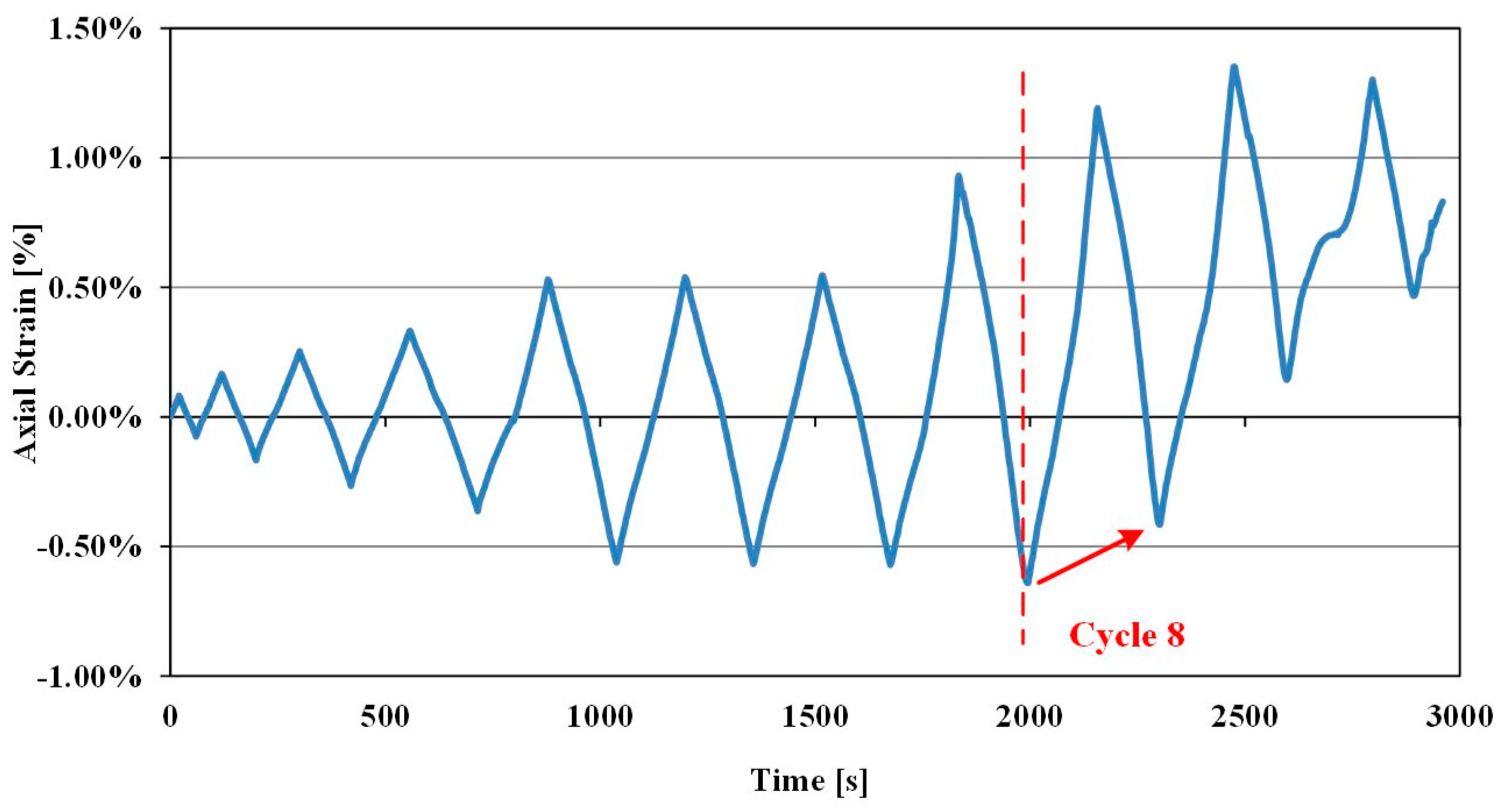
The adopted criterion for onset of buckling in the large-scale ULCF experiments [22] is a significant decrease of oscillation amplitude in axial strain from one half-cycle to the previous one in the reference position, as illustrated in Figure 17.
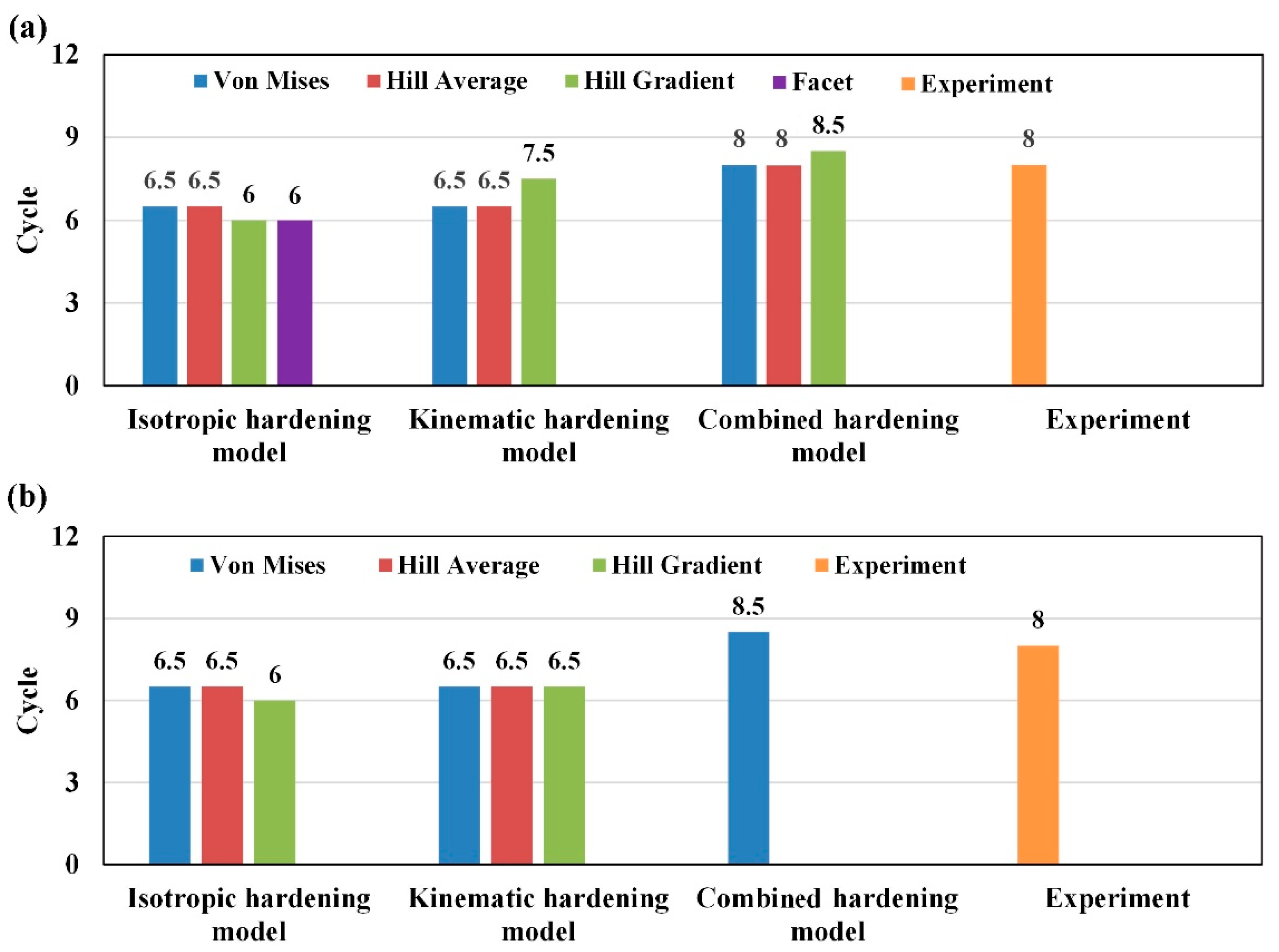
To test the influence of various plasticity modeling assumptions, simulations of the ULCF are performed using ABAQUS, and the results are compared to the stable experimental results with good repeatability in former work [22]. As the calculation with the facet method is available in explicit time integration schemes, in order to compare all of the results with different yield criteria in the same time integration scheme, both explicit and implicit time integration schemes are adopted in the FE simulations to firstly exclude the influence of time integration schemes on the results. A comparison of the number of cycles at onset of buckling is presented in Figure 18. It can be seen that for identical constitutive models, the onset of buckling is in nearly all cases predicted at the same cycle for both explicit (Figure 18a) and implicit (Figure 18b) FE integration schemes. This confirms that the physical phenomenon of ULCF buckling is captured, independent of the numerical implementation in the finite element simulation scheme. Comparing results for the various constitutive models, it is seen that the assumption of combined kinematic hardening leads to close agreement to the experiment, with only a small influence of the adopted yield function. Isotropic and linear kinematic hardening models give systematic under-prediction of the onset of buckling.
4.2. Strain Evolution
4.2.1. Influence of Anisotropic Yield Locus on Strain Evolution and Buckling Subjected to ULCF
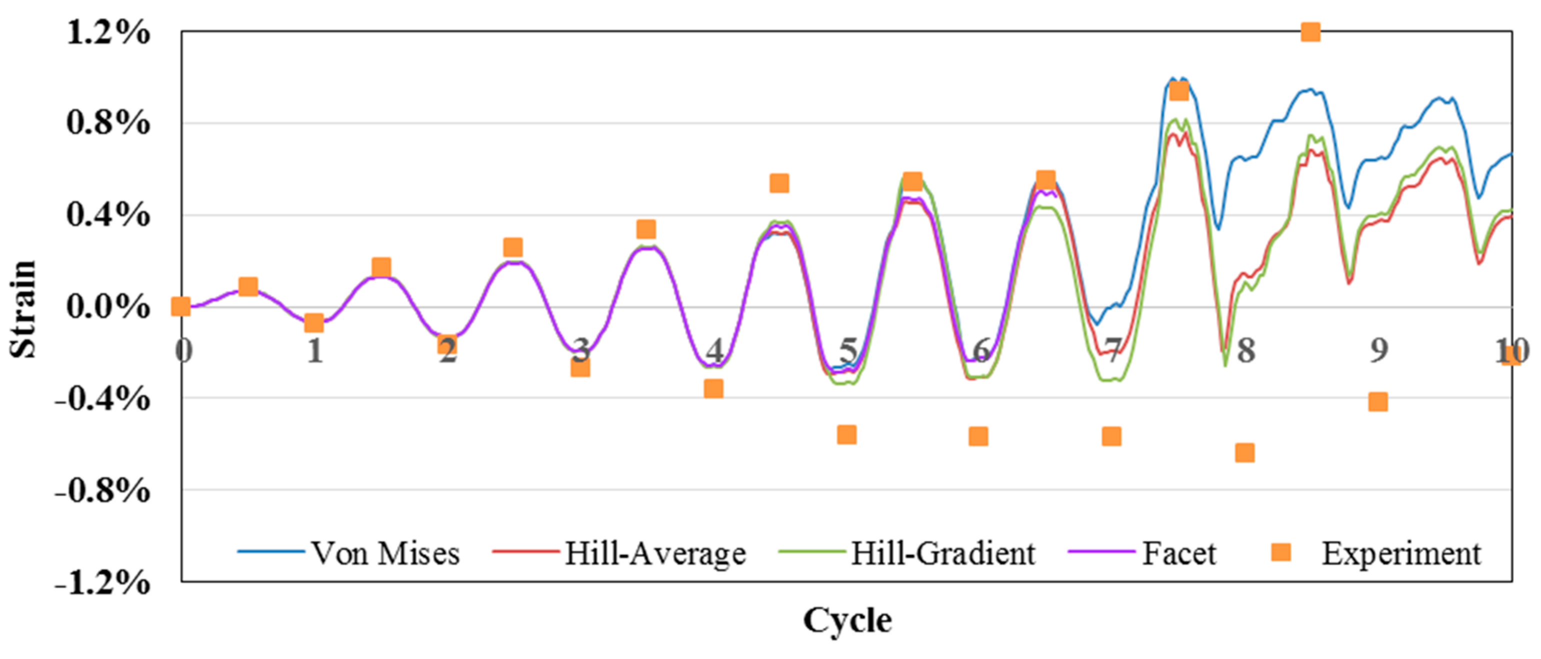
Figure 19, Figure 20, Figure 21, Figure 22 and Figure 23 compare the axial strain evolution of the experimental results at the reference position with those of the numerical simulations with different constitutive models. In all simulations, the occurrence of plastic deformation was captured all around the fourth cycle by the equivalent plastic strain values, resulting in the nearly same strain evolution before the fourth cycle. The differences of axial strain evolution with respect to various plastic models were discussed in terms of the plastic deformation before buckling.
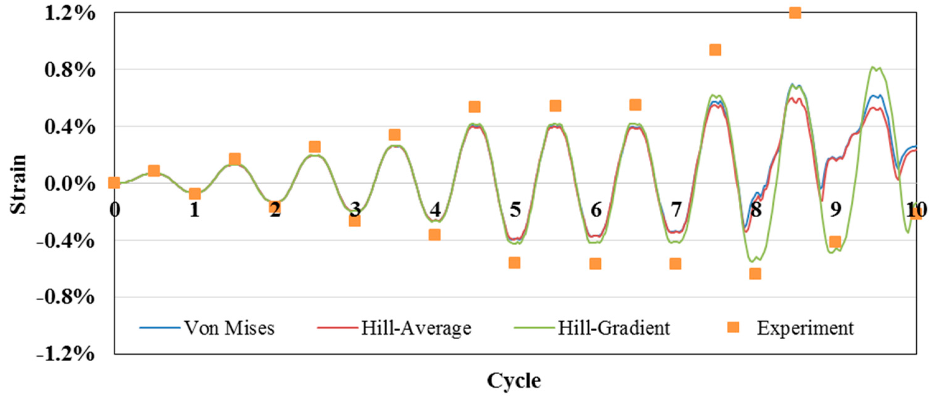
Simulations with different yield criteria taking into account combined hardening all resulted in buckling at the center of the pipe, respectively at the 8.5th cycle for Hill-gradient and the eight cycle for both von Mises and Hill-average. Accurate predictions of strain evolution for these models are obtained (Figure 19).
The experimentally-measured axial strain at 25 cm from the center was as a consequence a bit higher than in the simulation, and the strain-evolution predictions during the ULCF process assuming the Hill anisotropic model with gradient properties over thickness (Hill-gradient) are largest in magnitude and closer to the experiment values.
In BS8010 [25] and Gresnight [26], relationships are proposed to calculate the critical buckling strain from the pipe outer diameter (OD) and wall thickness (WT), independently of the strength of the tube material. Applied to the current geometry (OD = 220 mm and WT = 5.56 mm), the critical buckling strain amplitude is found to be 1.2%. Figure 20 shows the axial strain distribution and buckling with the Hill-gradient yield locus taking into account combined hardening at the 8.5th cycle, which coincides with the occurrence of buckling at the center of the pipe. It can be seen that in the central region with reduced thickness, the strain locally exceeds 1.2% and reaches 2.97%, and this validates the critical strain criterion for buckling proposed in [22].
Figure 21 compares the experimental axial strain at the reference position and the predicted ones for linear kinematic hardening with von Mises, Hill-average and Hill-gradient. Furthermore, in this case, the most accurate prediction of strain evolution before onset of buckling is realized by the Hill-gradient. A similar conclusion can be drawn comparing the different yield loci in combination with the isotropic hardening law in Figure 22.
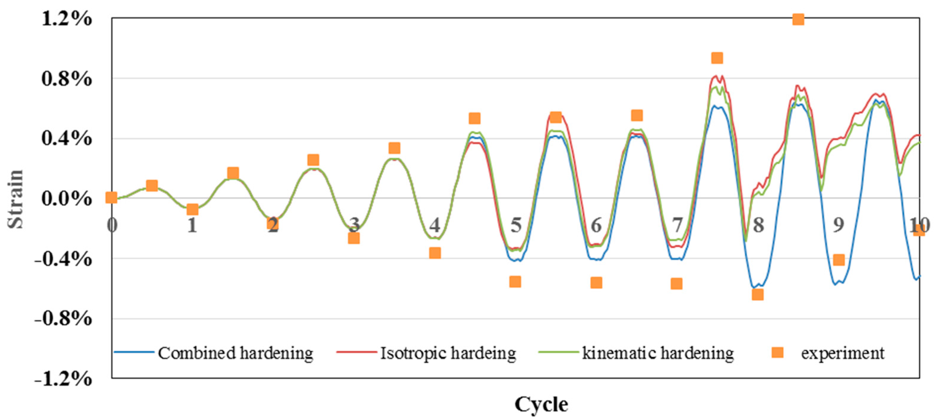
4.2.2. Influence of Strain Hardening on Strain Evolution and Buckling Subjected to ULCF with Hill-Gradient Anisotropic Yield Locus
Considering the comparatively accurate prediction of strain evolution with respect to the Hill-gradient anisotropic yield locus, the axial strain evolution under the Hill-gradient yield locus with different strain hardening models is presented again in Figure 23. The result confirms that the assumption of a combined hardening model delays the onset of buckling in ULCF, compared to isotropic and linear kinematic hardening models.
5. Summary and Conclusions
In this paper, a detailed experimental and numerical study of advanced plasticity modeling for ultra-low cycle fatigue simulation of steel pipe was presented. From the results of numerical simulations and experiments, the following conclusions are drawn:
- 1
- In terms of simulations with different strain-hardening models, the combined hardening model enables predicting accurately the onset of buckling. Compared to isotropic and linear kinematic hardening assumptions, the prediction of buckling is delayed with two bending cycles, resulting in eight or 8.5 cycles in total for the ULCF test setup under consideration, whereas eight cycles are experimentally found.
- 2
- Regarding the yield function assumption, it is systematically found that strain evolution predictions during the ULCF process are closest in agreement with the experiment for the Hill anisotropic model that accounts for the gradient in properties over the tube wall thickness.
- 3
- A significant texture gradient across thickness is observed. The texture anisotropy gradient has an obvious effect on the strain evolution of ULCF simulation and to some degree also on the buckling failure process.
- 4
- Hardening modeling matters more than modeling assumptions regarding the (an-)isotropy (i.e., the choice and calibration of the yield locus) in the simulation of pipeline steel undergoing ULCF.
Acknowledgments
Authors Philip Eyckens and Albert Van Bael gratefully acknowledge the financial support of the Industrieel Onderzoeksfonds of KU Leuven (Project C32/15/017). The author Rongting Li wishes to acknowledge the scholarship of China Scholarship Council to study at KU LEUVEN for one year, gratefully thanks Prof. Van Bael, Philip Eyckens and Jerzy Gawad for all of the guidance in the one year’s study and acknowledges Maarten Van Poucke and Steven Cooreman for the former experimental work and simulation research of the ULCF test.
Author Contributions
Rongting Li performed the sample preparation, finite element simulation data analysis and manuscript writing and editing. Maarten Van Poucke and Steven Cooreman contributed to the lab ultra-low cycle fatigue (ULCF) test and the test analysis. Jerzy Gawad contributed to the computational technology support. Philip Eyckens, Daxin E and Albert Van Bael contributed to program supervision and manuscript revision.
Conflicts of Interest
The authors declare no conflicts of interest.
References
- Prager, W. Recent developments in the mathematical theory of plasticity. J. Appl. Phys. 1949, 20, 235–241. [Google Scholar] [CrossRef]
- Wu, H.-C. Anisotropic plasticity for sheet metals using the concept of combined isotropic-kinematic hardening. Int. J. Plast. 2002, 18, 1661–1682. [Google Scholar] [CrossRef]
- Chung, K.; Lee, M.-G.; Kim, D.; Kim, C.; Wenner, M.L.; Barlat, F. Spring-back evaluation of automotive sheets based on isotropic-kinematic hardening laws and non-quadratic anisotropic yield functions. Int. J. Plast. 2005, 21, 861–882. [Google Scholar] [CrossRef]
- Hill, R. A theory of the yielding and plastic flow of anisotropic metals. Proc. R. Soc. Lond. 1948, 193, 281–297. [Google Scholar] [CrossRef]
- Mises, R.V. Mechanik der plastischen formänderung von kristallen. ZAMM J. Appl. Math. Mech./Z. Angew. Math. Mech. 1928, 8, 161–185. [Google Scholar] [CrossRef]
- Barlat, F.; Ferreira, D.J.M.; Gracio, J.J.; Lopes, A.B.; Rauch, E.F. Plastic flow for non-monotonic loading conditions of an aluminum alloy sheet sample. Int. J. Plast. 2003, 19, 1215–1244. [Google Scholar] [CrossRef]
- Yoon, J.W.; Barlat, F.; Dick, R.E.; Karabin, M.E. Prediction of six or eight ears in a drawn cup based on a new anisotropic yield function. Int. J. Plast. 2006, 22, 174–193. [Google Scholar] [CrossRef]
- Comsa, D.S; Banabic, D. Plane-Stress Yield Criterion for Highly-Anisotropic Sheet Metals; Numisheet 2008: Interlaken, Switzerland, 2008; pp. 43–48. [Google Scholar]
- Plunkett, B.; Cazacu, O.; Barlat, F. Orthotropic yield criteria for description of the anisotropy in tension and compression of sheet metals. Int. J. Plast. 2008, 24, 847–866. [Google Scholar] [CrossRef]
- Van Houtte, P.; Yerra, S.K.; Van Bael, A. The facet method: A hierarchical multilevel modelling scheme for anisotropic convex plastic potentials. Int. J. Plast. 2009, 25, 332–360. [Google Scholar] [CrossRef]
- Van Houtte, P.; Kanjarla, A.K.; Van Bael, A.; Seefeldt, M.; Delannay, L. Multiscale modelling of the plastic anisotropy and deformation texture of polycrystalline materials. Eur. J. Mech. A/Solids 2006, 25, 634–648. [Google Scholar] [CrossRef]
- Van Houtte, P.; Gawad, J.; Eyckens, P.; Van Bael, B.; Samaey, G.; Roose, D. Multi-scale modelling of the development of heterogeneous distributions of stress, strain, deformation texture and anisotropy in sheet metal forming. Procedia IUTAM 2012, 3, 67–75. [Google Scholar] [CrossRef]
- Gawad, J.; Van Bael, A.; Eyckens, P.; Samaey, G.; Van Houtte, P.; Roose, D. Hierarchical multi-scale modeling of texture induced plastic anisotropy in sheet forming. Comput. Mater. Sci. 2013, 66, 65–83. [Google Scholar] [CrossRef]
- Eyckens, P.; Mulder, H.; Gawad, J.; Vegter, H.; Roose, D.; van den Boogaard, T.; Van Bael, A.; Van Houtte, P. The prediction of differential hardening behaviour of steels by multi-scale crystal plasticity modelling. Int. J. Plast. 2015, 73, 119–141. [Google Scholar] [CrossRef]
- Gawad, J.; Banabic, D.; Van Bael, A.; Comsa, D.S.; Gologanu, M.; Eyckens, P.; Van Houtte, P.; Roose, D. An evolving plane stress yield criterion based on crystal plasticity virtual experiments. Int. J. Plast. 2015, 75, 141–169. [Google Scholar] [CrossRef]
- Gawad, J.; Banabic, D.; Comsa, D.S.; Gologanu, M.; Van Bael, A.; Eyckens, P.; Van Houtte, P.; Roose, D. Evolving Texture-Informed Anisotropic Yield Criterion for Sheet Forming. AIP Conf. Proc. 2013, 1567, 350–355. [Google Scholar]
- Kanvinde, A.M. Micromechanical Simulation of Earthquake-Induced Fracture in Steel Structures. Available online: http://adsabs.harvard.edu/abs/2004PhDT.......249K (accessed on 5 March 2017).
- Xue, L. A unified expression for low cycle fatigue and extremely low cycle fatigue and its implication for monotonic loading. Int. J. Fatigue 2008, 30, 1691–1698. [Google Scholar] [CrossRef]
- Campbell, F.C. Elements of Metallurgy and Engineering Alloys; ASM International: Geauga County, OH, USA, 2008. [Google Scholar]
- Lubliner, J.; Oliver, J.; Oller, S.; Oñate, E. A plastic-damage model for concrete. Int. J. Solids Struct. 1989, 25, 299–326. [Google Scholar] [CrossRef]
- Martinez, X.; Oller, S.; Barbu, L.G.; Barbat, A.H.; Jesus, A.M.P.D. Analysis of ultra low cycle fatigue problems with the barcelona plastic damage model and a new isotropic hardening law. Int. J. Fatigue 2015, 73, 132–142. [Google Scholar] [CrossRef]
- European Commission. Ultra Low Cycle Fatigue of Steel under Cyclic High-Strain Loading Conditions (ULCF). Available online: http://bookshop.europa.eu/en/ultra-low-cycle-fatigue-of-steel-under-cyclic-high-strain-loading-conditions-ulcf--pbKINA27731/ (accessed on 5 March 2017).
- Vanhoutte, P. Deformation texture prediction: From the taylor model to the advanced lamel model. Int. J. Plast. 2005, 21, 589–624. [Google Scholar] [CrossRef]
- Van Houtte, P. The MTM-FHM Software System Version 2; MTM-KU: Leuven, Belgium, 1995. [Google Scholar]
- Institution, British Standards. Code of Practice for Pipelines. Pipelines Subsea: Design, Construction and Installation. Available online: http://shop.bsigroup.com/ProductDetail/?pid=000000000000289228 (accessed on 5 March 2017).
- Gresnigt, A.M.; Foeken, R.J.V. Local Buckling of Uoe and Seamless Steel Pipes. In Proceedings of the Eleventh International Offshore and Polar Engineering Conference, Stavanger, Norway, 17–22 June 2001. [Google Scholar]
Figure 1.
The experimental bending setup of ultra-low cycle fatigue (ULCF) [22].
Figure 1.
The experimental bending setup of ultra-low cycle fatigue (ULCF) [22].
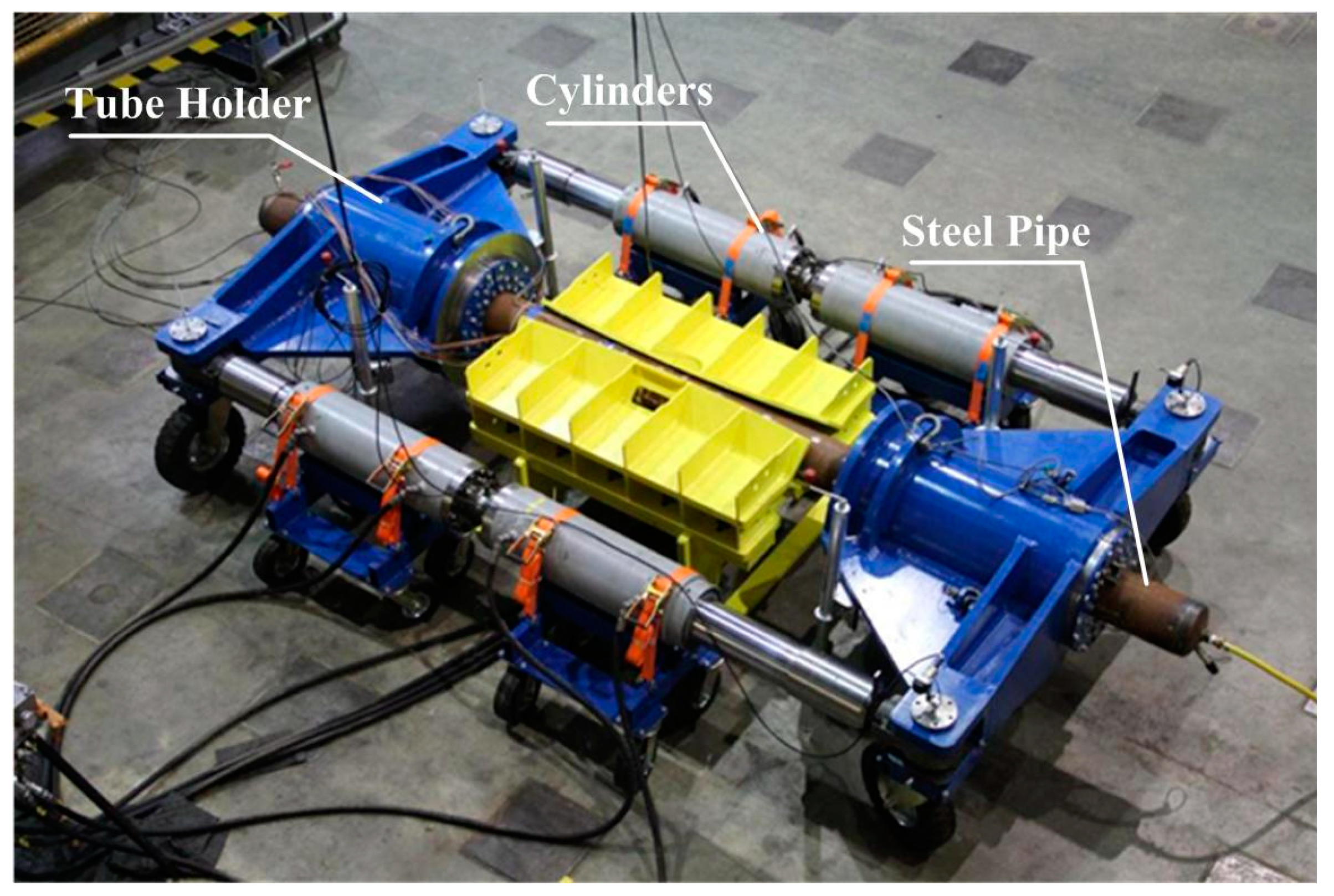
Figure 2.
The geometry of the ULCF in ABAQUS FE model, with four reference points (RP) for defining the boundary conditions.
Figure 2.
The geometry of the ULCF in ABAQUS FE model, with four reference points (RP) for defining the boundary conditions.
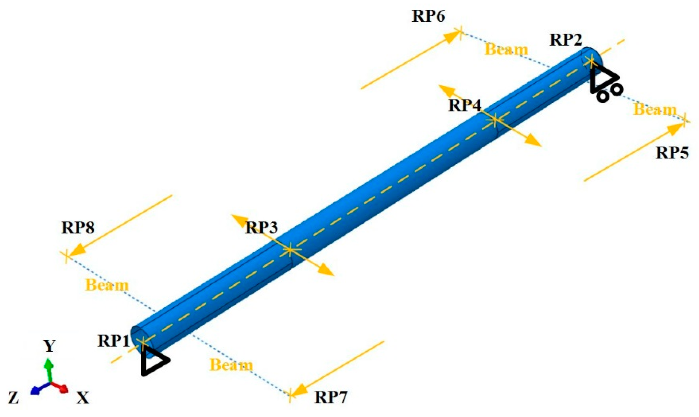
Figure 3.
Schematic of the cyclic load pattern.
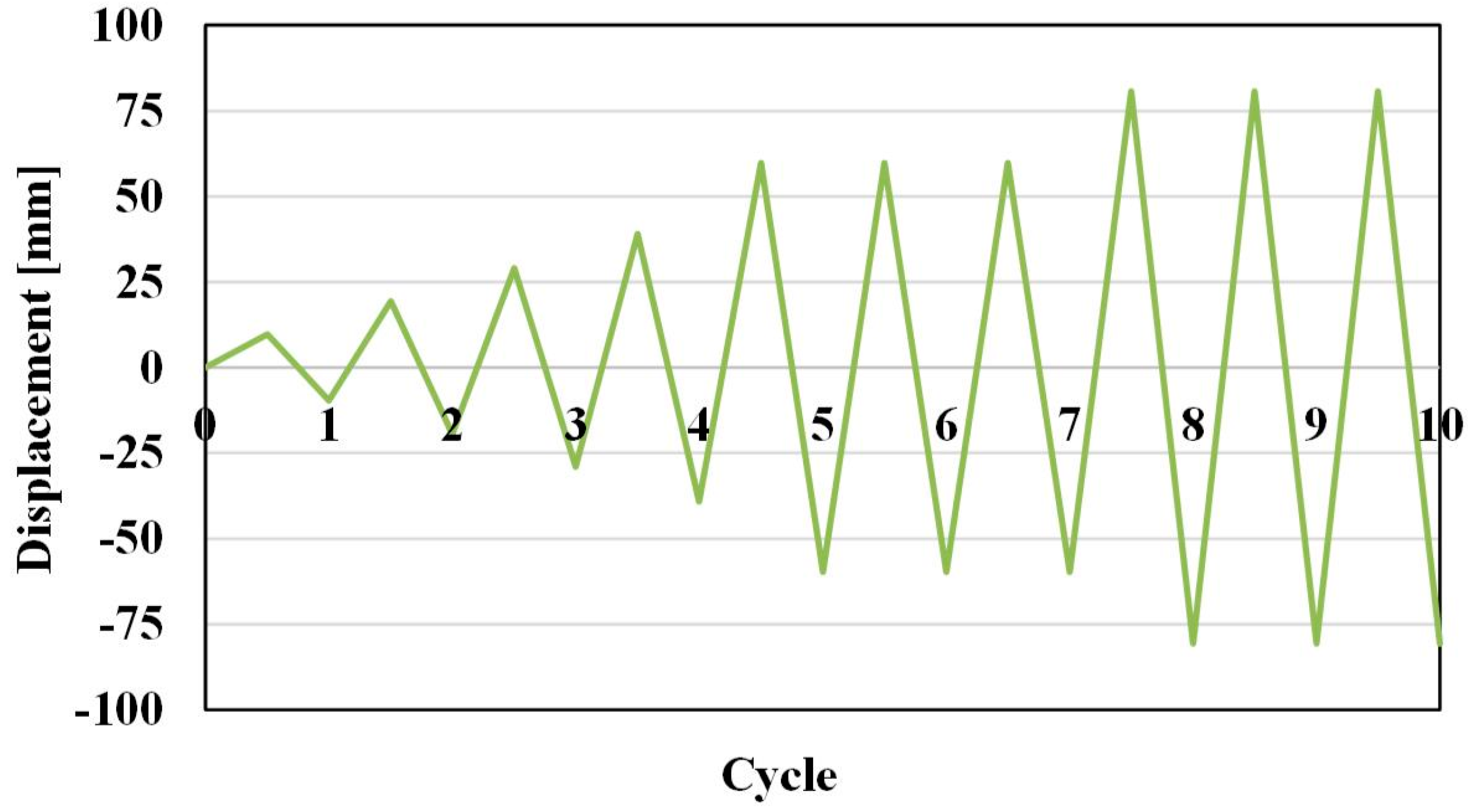
Figure 4.
Geometry and dimensions of the experimental pipe.
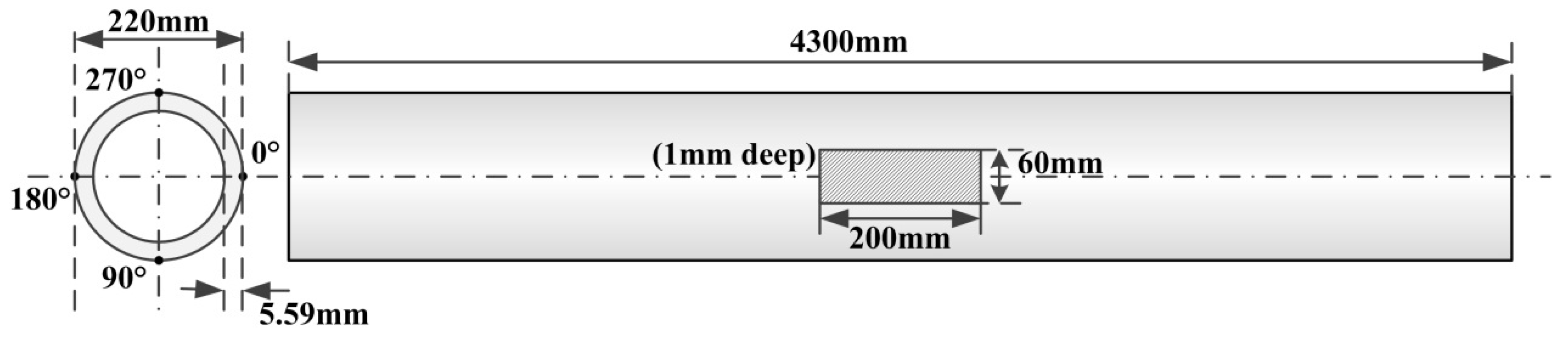
Figure 5.
The optical microstructure of X65 steel: (a,b) in the weld zone; (c,d) 90° to welding.

Figure 6.
The applied stress-strain behavior obtained from monotonic tensile tests along the tube axial direction.
Figure 6.
The applied stress-strain behavior obtained from monotonic tensile tests along the tube axial direction.
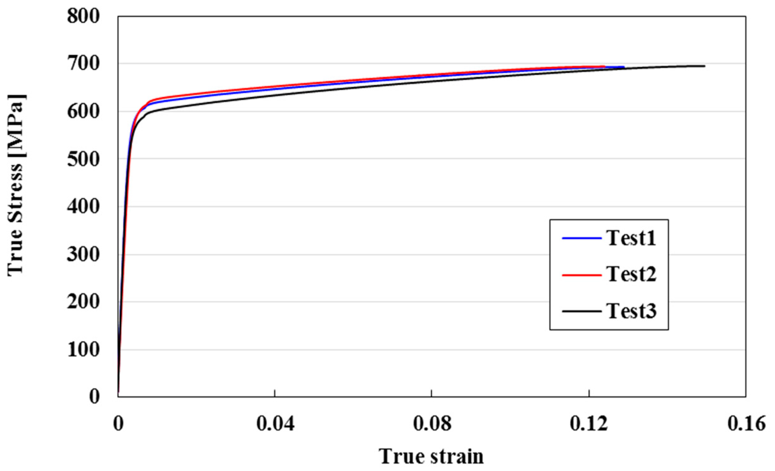
Figure 7.
Results of cyclic tension-compression tests: (a) the true stress-strain curve under strain different amplitudes and (b) changes in stress at the end of tension and compression as a function of the number of cycles.
Figure 7.
Results of cyclic tension-compression tests: (a) the true stress-strain curve under strain different amplitudes and (b) changes in stress at the end of tension and compression as a function of the number of cycles.

Figure 8.
2 = 45° orientation distribution function (ODF) sections of the initial texture of the material at different locations.
Figure 8.
2 = 45° orientation distribution function (ODF) sections of the initial texture of the material at different locations.
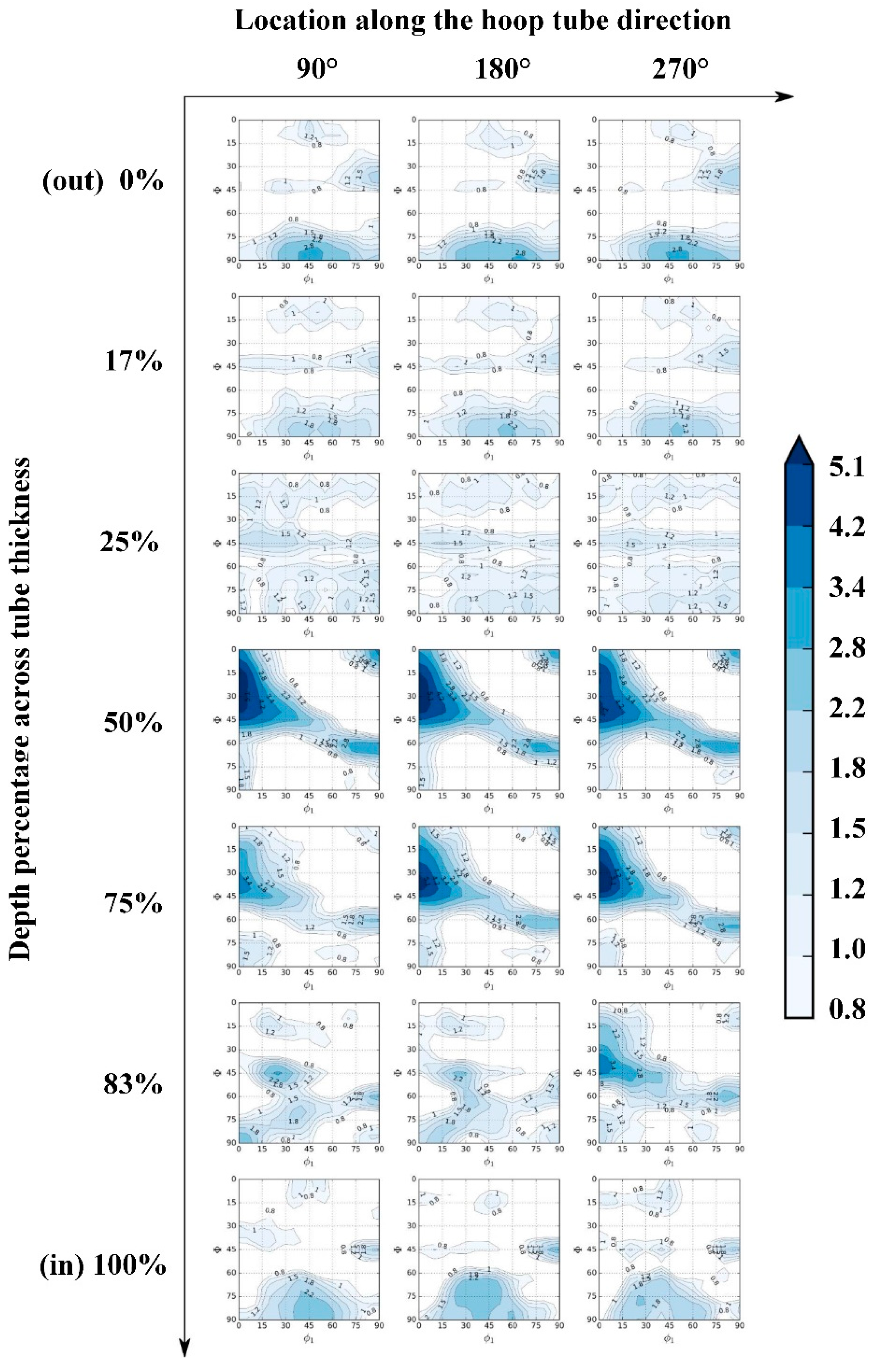
Figure 9.
The texture index at different locations.

Figure 10.
2 = 45° ODF sections of the merged textures along the hoop (positions 90°, 180° and 270°) (first row) and the ODF section of the overall merged texture (second row).
Figure 10.
2 = 45° ODF sections of the merged textures along the hoop (positions 90°, 180° and 270°) (first row) and the ODF section of the overall merged texture (second row).
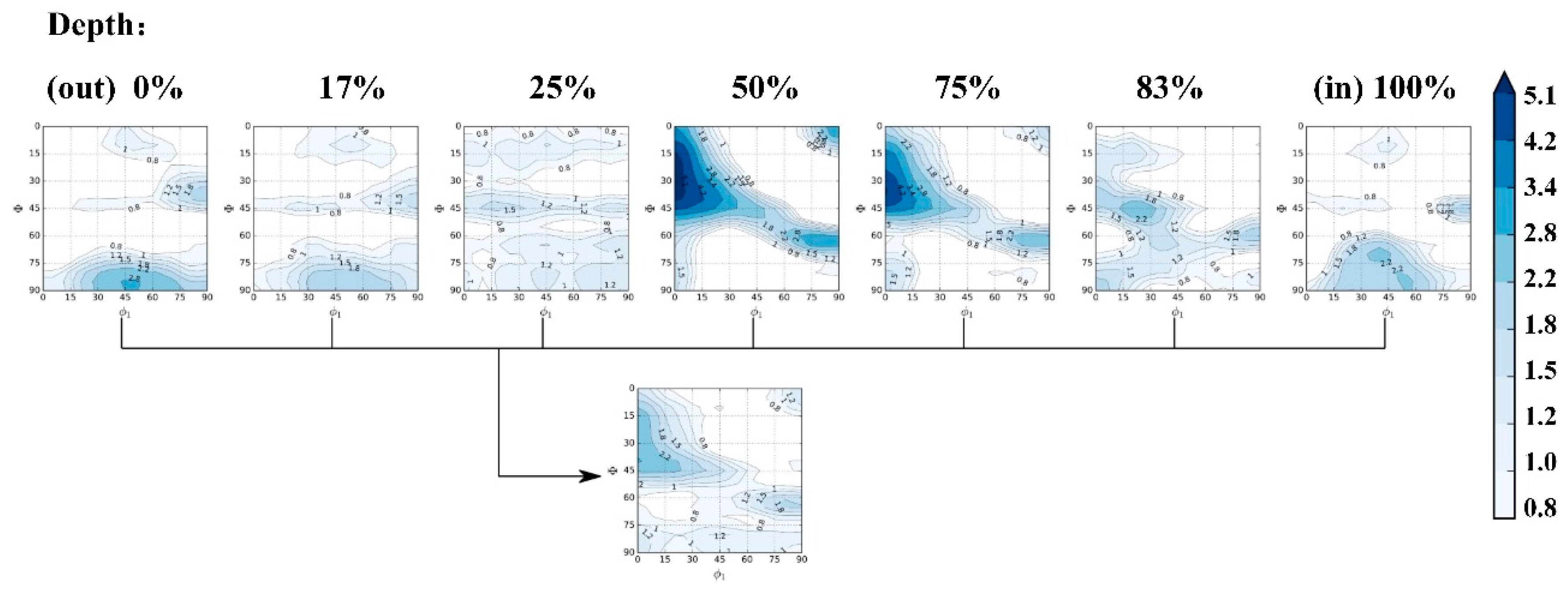
Figure 11.
Two-dimensional sections of the yield surfaces calibrated by VEF.

Figure 12.
The diagram of the material definition in ABAQUS with the Hill-gradient yield locus.
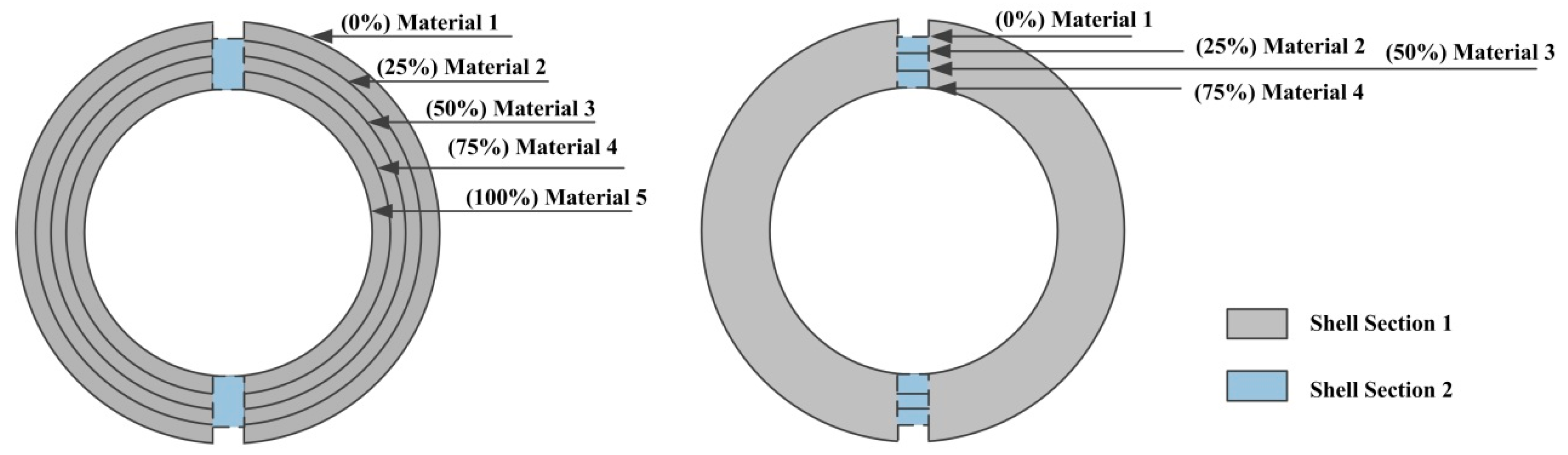
Figure 13.
The r-values corresponding to the merged texture data at five different depths across tube thickness calibrated by VEF.
Figure 13.
The r-values corresponding to the merged texture data at five different depths across tube thickness calibrated by VEF.

Figure 14.
Two-dimensional sections of the yield surfaces calibrated by VEF at 0%, 25%, 50%, 75% and 100% across the thickness.
Figure 14.
Two-dimensional sections of the yield surfaces calibrated by VEF at 0%, 25%, 50%, 75% and 100% across the thickness.

Figure 15.
Two-dimensional sections of the yield surfaces respectively calibrated by the VEF/facet method.
Figure 15.
Two-dimensional sections of the yield surfaces respectively calibrated by the VEF/facet method.
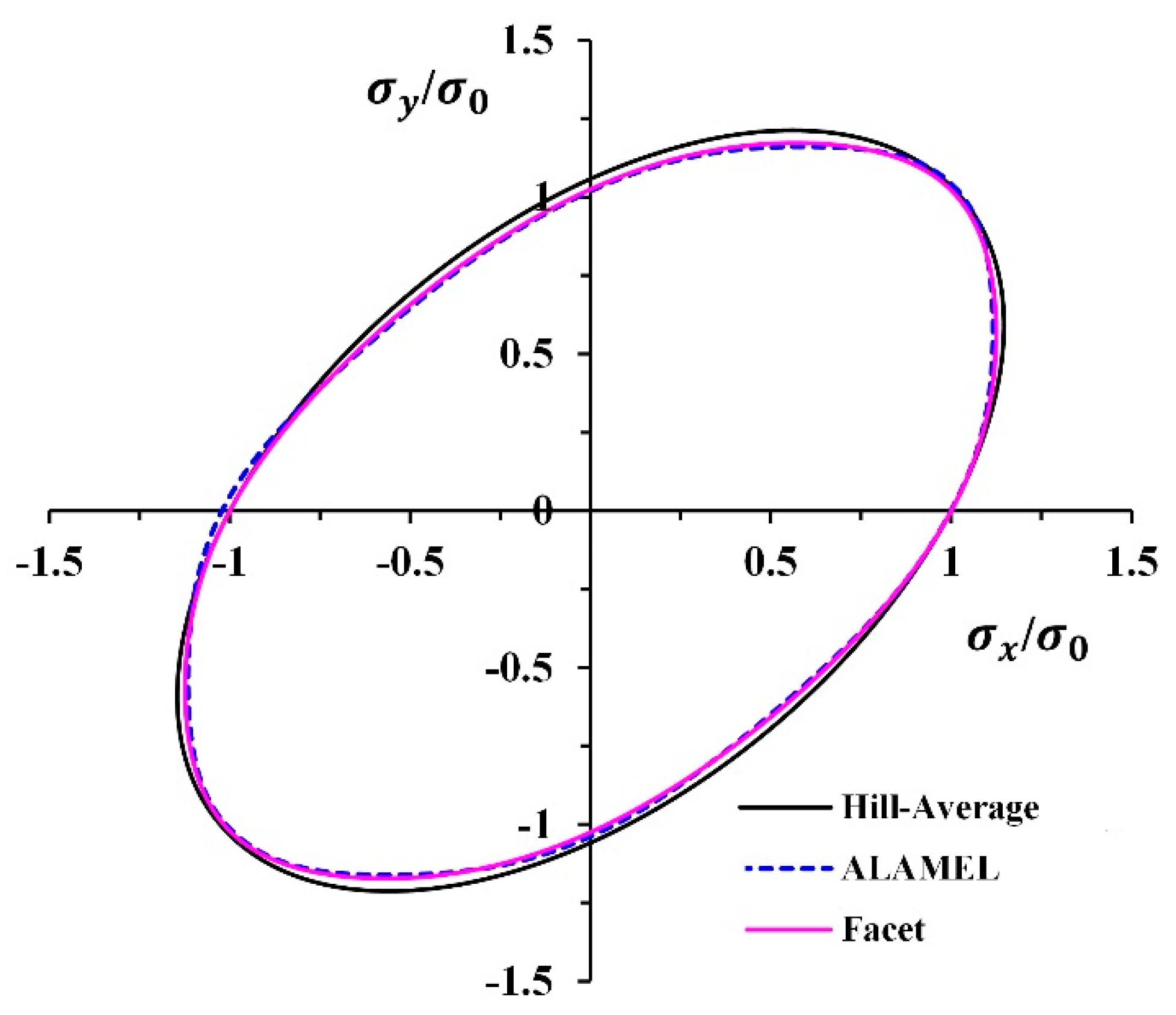
Figure 16.
The reference position for tracking strain evolution in the experiment and simulation.
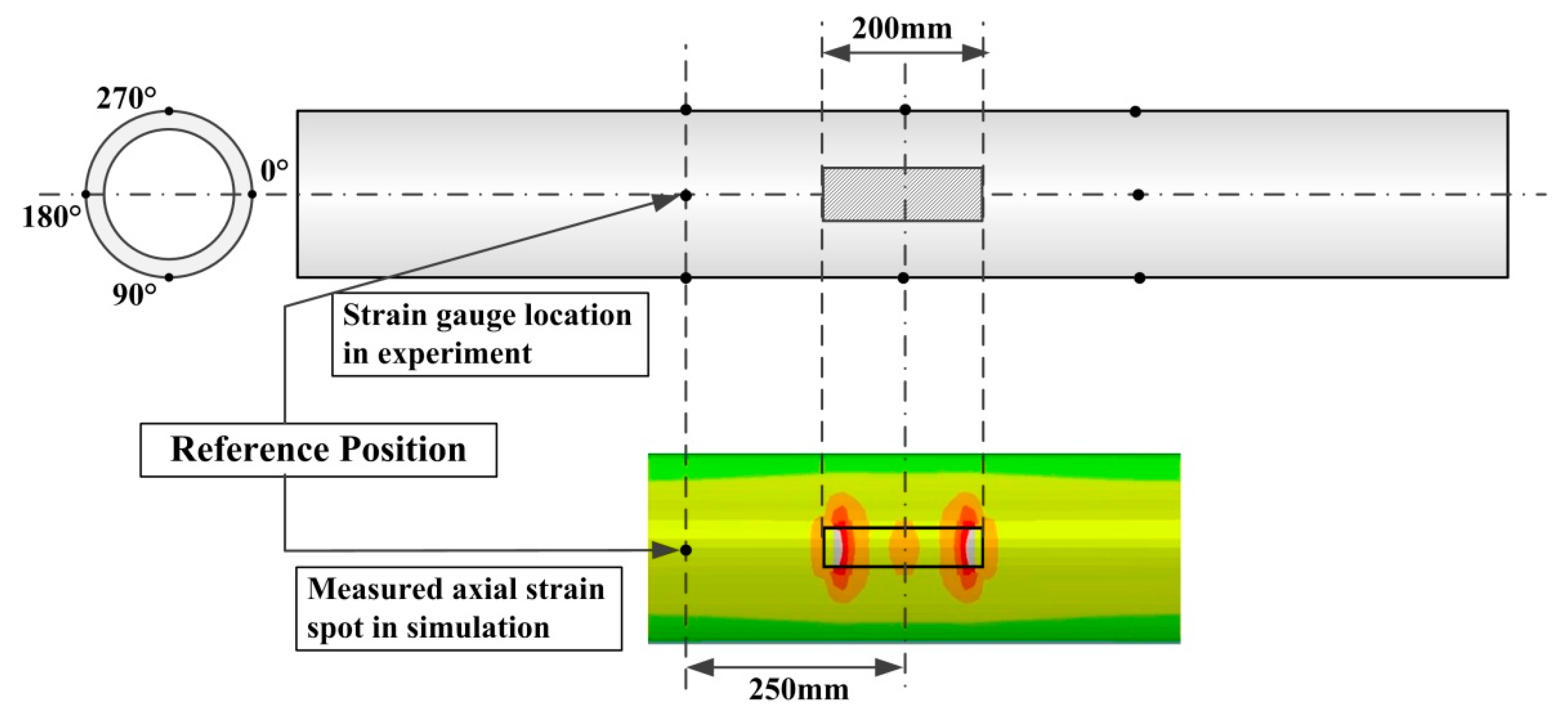
Figure 17.
Illustration of the criterion for determining the onset of buckling. Experimental measurement data of axial strain in the reference position [22].
Figure 17.
Illustration of the criterion for determining the onset of buckling. Experimental measurement data of axial strain in the reference position [22].

Figure 18.
Comparison of prediction of the onset of buckling to the experiment for (a) explicit and (b) implicit FE simulations.
Figure 18.
Comparison of prediction of the onset of buckling to the experiment for (a) explicit and (b) implicit FE simulations.

Figure 19.
Axial strain evolution in explicit time integration FE simulation with the combined hardening model.
Figure 19.
Axial strain evolution in explicit time integration FE simulation with the combined hardening model.

Figure 20.
Axial strain and buckling overview at the 8.5th cycle with combined hardening and the Hill-gradient yield locus.
Figure 20.
Axial strain and buckling overview at the 8.5th cycle with combined hardening and the Hill-gradient yield locus.
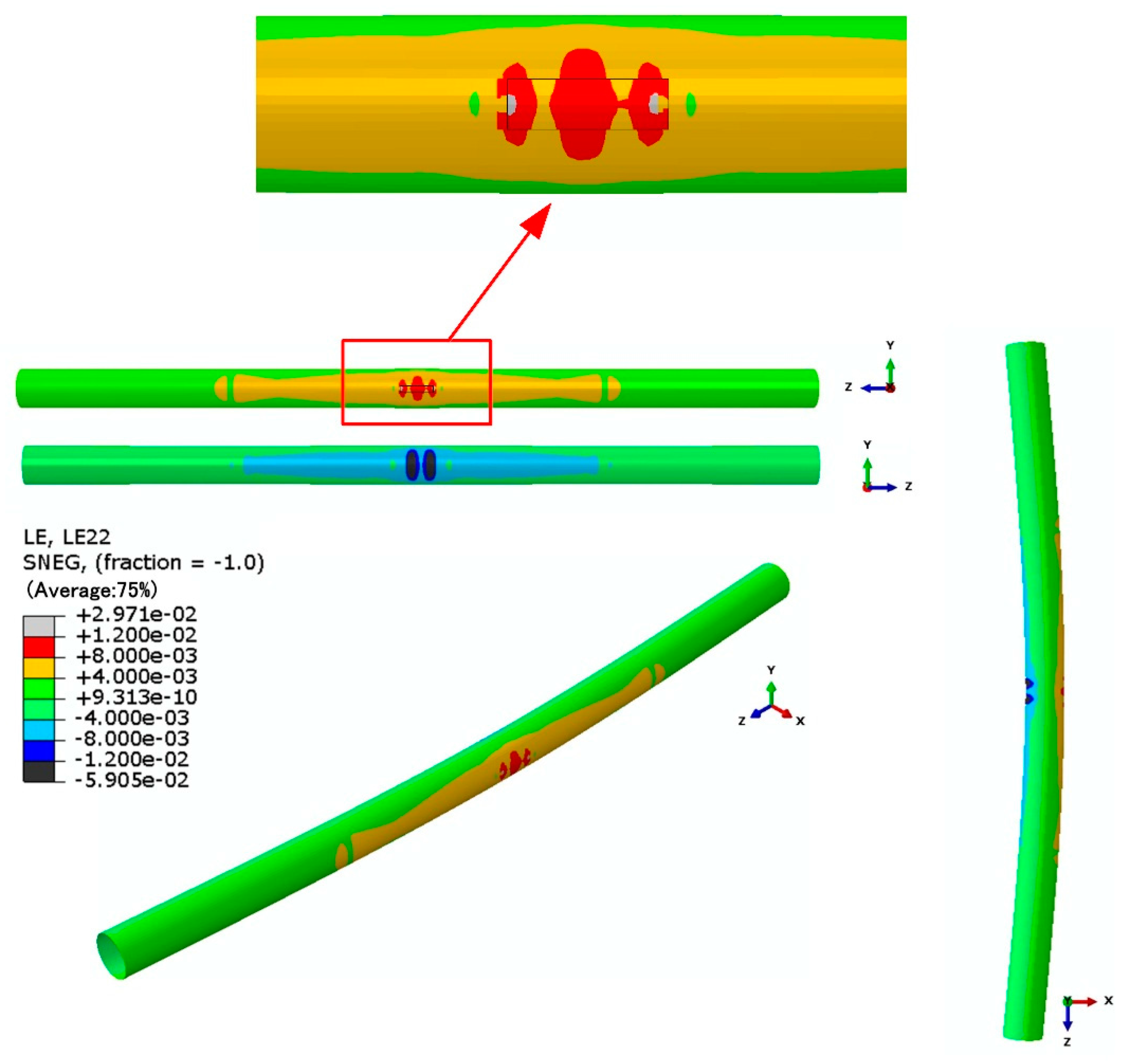
Figure 21.
Axial strain evolution in explicit calculation with the linear kinematic hardening model.
Figure 21.
Axial strain evolution in explicit calculation with the linear kinematic hardening model.
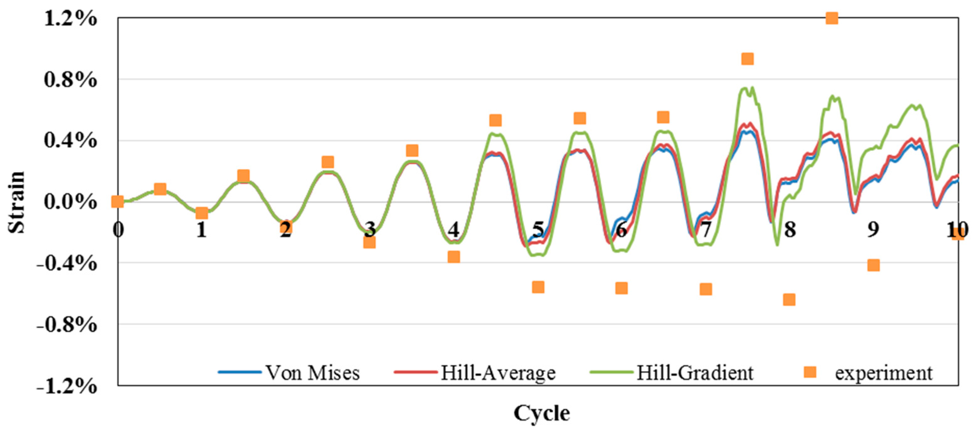
Figure 22.
Axial strain evolution in explicit calculation with the isotropic hardening model.

Figure 23.
Axial strain evolution in explicit calculation with different hardening models.


Table 1.
Material parameters corresponding to the isotropic hardening law, linear kinematic hardening law and combined hardening law.
Table 1.
Material parameters corresponding to the isotropic hardening law, linear kinematic hardening law and combined hardening law.
| Hardening Law | Material Parameters | |||
|---|---|---|---|---|
| (MPa) | Tabular Data | |||
| Isotropic hardening | --- | --- | = 760 MPa | |
| B = 0.05 | ||||
| Linear kinematic hardening | 594 | 0 | = 656 MPa | |
| 678 | 0.128 | |||
| Combined hardening | Nonlinear kinematic hardening component | --- | --- | = 600 MPa |
| = 49,376 MPa | ||||
| = 234.351 | ||||
| Isotropic hardening component | 600 | 0 | --- | |
| 444 | 0.044 | |||
| 512 | 1 | |||
Table 2.
r-values calibrated by VEF based on the ALAMEL model.
| r Value of Overall Merged Texture | |||
|---|---|---|---|
| ALAMEL | r0 | r45 | r90 |
| 0.858 | 1.250 | 1.070 | |
© 2017 by the authors. Licensee MDPI, Basel, Switzerland. This article is an open access article distributed under the terms and conditions of the Creative Commons Attribution (CC BY) license (http://creativecommons.org/licenses/by/4.0/).
Share and Cite
MDPI and ACS Style
Li, R.; Eyckens, P.; E, D.; Gawad, J.; Poucke, M.V.; Cooreman, S.; Bael, A.V. Advanced Plasticity Modeling for Ultra-Low-Cycle-Fatigue Simulation of Steel Pipe. Metals 2017, 7, 140. https://doi.org/10.3390/met7040140
AMA Style
Li R, Eyckens P, E D, Gawad J, Poucke MV, Cooreman S, Bael AV. Advanced Plasticity Modeling for Ultra-Low-Cycle-Fatigue Simulation of Steel Pipe. Metals. 2017; 7(4):140. https://doi.org/10.3390/met7040140
Chicago/Turabian StyleLi, Rongting, Philip Eyckens, Daxin E, Jerzy Gawad, Maarten Van Poucke, Steven Cooreman, and Albert Van Bael. 2017. "Advanced Plasticity Modeling for Ultra-Low-Cycle-Fatigue Simulation of Steel Pipe" Metals 7, no. 4: 140. https://doi.org/10.3390/met7040140
Note that from the first issue of 2016, this journal uses article numbers instead of page numbers. See further details here.