Effect of Constitutive Equations on Springback Prediction Accuracy in the TRIP1180 Cold Stamping

1
Division of Precision and Manufacturing Systems, Pusan National University, Busandaehak-ro 63beon-gil, Geumjeong-gu, Busan 609-735, Korea
2
Press Die Research Team, Nara Mold & Die Co. Ltd., Gongdan-ro 675, Seongsan-gu, Changwon-City, Gyeongnam 642-120, Korea
3
School of Mechanical Engineering, Pusan National University, Busandaehak-ro 63beon-gil, Geumjeong-gu, Busan 609-735, Korea
*
Author to whom correspondence should be addressed.
Metals 2018, 8(1), 18; https://doi.org/10.3390/met8010018
Submission received: 30 October 2017
/
Revised: 21 November 2017
/
Accepted: 25 December 2017
/
Published: 30 December 2017
(This article belongs to the Special Issue Advances in Plastic Forming of Metals)
Abstract
:This study aimed to evaluate the effect of constitutive equations on springback prediction accuracy in cold stamping with various deformation modes. This study investigated the ability of two yield functions to describe the yield behavior: Hill’48 and Yld2000-2d. Isotropic and kinematic hardening models based on the Yoshida-Uemori model were adopted to describe the hardening behavior. The chord modulus model was used to calculate the degradation of the elastic modulus that occurred during plastic loading. Various material tests (such as uniaxial tension, tension-compression, loading-unloading, and hydraulic bulging tests) were conducted to determine the material parameters of the models. The parameters thus obtained were implemented in a springback prediction finite element (FE) simulation, and the results were compared to experimental data. The springback prediction accuracy was evaluated using U-bending and T-shape drawing. The constitutive equations wielded significant influence over the springback prediction accuracy. This demonstrates the importance of selecting appropriate constitutive equations that accurately describe the material behaviors in FE simulations.
1. Introduction
In recent years, lightweight vehicles have gained attention as fuel efficiency and gas emission regulations become increasingly stringent [1]. As weight reduction has become a key goal, many researchers have devoted significant efforts to selecting the materials for manufacturing automotive parts. Advanced high strength steel (AHSS) has been widely used in the automotive industry for its light weight, crashworthiness, and productivity. However, it is difficult to achieve dimensional accuracy with AHSS because its higher elastic recovery and yield strength cause excessive springback [2]. Fabricating a target product shape with AHSS is challenging for part manufacturers, requiring a considerable amount of time as well as additional costs to modify tools for this springback.
Finite element (FE) simulation may be applied to describe AHSS material behaviors and springback, as this provides a cost-effective and reliable method for predicting springback. The constitutive equations used in FE simulations strongly influence the accuracy of the prediction results. Thus, many researchers have suggested varying constitutive equations. Multiple equations have been used to describe the hardening behavior of AHSS, including the nonlinear kinematic hardening model proposed by Chaboche [3], the kinematic hardening model based on cyclic plasticity suggested by Yoshida, and the distortional hardening model recommended by Barlat. In addition, Hill’48 and Yld2000-2d have been widely used to model the anisotropic behavior of AHSS.
Many published studies have investigated the influence of constitutive equations on simulated prediction results. Lee et al. [4] performed a springback evaluation of automotive sheets based on an isotropic kinematic hardening model and anisotropic yield functions. It was found that the hardening behaviors, including Bauschinger and transient elements, were well represented by the modified Chaboche model. Furthermore, the work-hardening data for dual phase steel (DP steel) was found to better conform to a power law-type hardening law than to the Voce-type law. Zang et al. [5] developed an elasto-plastic constitutive model based on one-surface plasticity. Their results demonstrated that the resulting material model is able to accurately predict springback when materials show a constant offset in permanent softening. Furthermore, Larsson et al. [6] concluded that neither isotropic nor kinematic hardening models were sufficient to describe the plastic-hardening behavior seen in non-linear strain paths. Thus, Larsson employed a combined isotropic-kinematic hardening model to evaluate the effects of springback in steel sheets. Eggertsen et al. [7] predicted the springback using various hardening models and yield functions. The Yoshida-Uemori hardening model has been shown to yield results that fit experimental measurements better than other options. Kim et al. [8] performed die compensation based on the Yld2000-2d yield function and Yoshida-Uemori hardening model. It was concluded that the dimensional accuracy of AHSS products can be achieved efficiently through die compensation using the material models in the multi-stage stamping process. Previous studies have demonstrated that the descriptions of anisotropic behavior, the Bauschinger effect, transient behavior, and the permanent softening effect are important. Successful springback prediction via FE simulation is principally dependent on selecting accurate yield criterion, hardening models, and material coefficients [9]. However, the above studies dealt with simply configured products such as those used in U-bending tests [10] and did not focus on AHSS products with various deformation modes. Therefore, it is necessary to evaluate the effect of the constitutive equations on springback prediction accuracy in AHSS cold stamping with multiple deformation modes.
The objective of this study was to evaluate the effect of constitutive equations on springback prediction accuracy in TRIP1180 cold stamping. In this study, two types of yield function were considered to describe the yield behavior: Hill’48 and the Yld2000-2d. Isotropic and kinematic hardening models based on the Yoshida-Uemori model were also adopted to describe the hardening behavior. The chord modulus model was utilized in the FE simulation alongside the hardening model constants. Various material tests, such as uniaxial tension, tension–compression, loading–unloading, and hydraulic bulging tests were conducted to determine material parameters for the models. The obtained parameters were utilized in the FE simulation to predict springback, and the results were compared with experimental data. In addition, U-bending and T-shape drawing were employed to evaluate the accuracy of the springback predictions.
2. Constitutive Equations for the TRIP1180 Sheet Steel
A TRIP1180 steel sheet with a thickness of 1.0 mm was investigated in this study. The TRIP1180 was used as received. The constitutive equations Hill’48 and Yld2000-2d were used to describe its yield behavior. Moreover, isotropic and kinematic hardening models based on the Yoshida-Uemori model were adopted to express hardening behavior. The chord modulus model was used to describe the degradation of the elastic modulus that occurs during plastic loading. The material constants of TRIP1180 for the constitutive equations were obtained from uniaxial tension, tension-compression, loading-unloading, and hydraulic bulging tests.
2.1. Yield Function
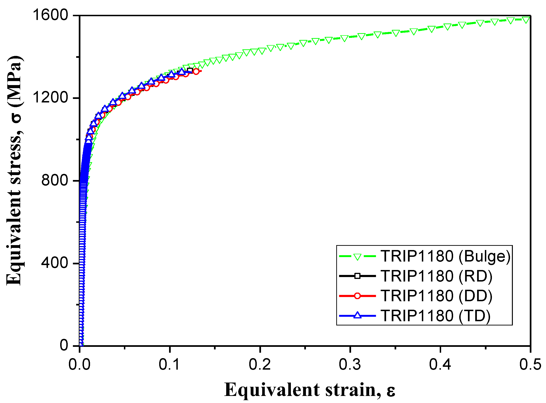
Yield functions define the transition of a material from elastic to plastic behavior in complex stress states. In this study, the Hill’48 and Yld2000-2d yield functions were used to evaluate the anisotropic yield behavior of TRIP1180. In order to determine the material parameters of the yield functions, ASTM E8 standard uniaxial tension tests were performed on specimens using a MTS universal testing machine for different rolling directions (0°, 45°, 90°), and hydraulic bulge tests were conducted to obtain a stable biaxial stress-strain curve with an Erichsen bulge tester. The biaxial yield stress and biaxial anisotropic plasticity coefficients were derived from the developed curve. A mechanical measurement device was placed on the top of the specimen to allow in-plane elongation and curvature measurements using an extensometer. The membrane stress and thickness strain were calculated using these measurements as described in the literature [11]. The yield stress in balanced biaxial tension () was calculated based on the work-equivalence principle by comparing the bulge and uniaxial tension flow curves. The results of these tests are shown in Figure 1.
2.1.1. Hill’48 Yield Function
The anisotropic yield criterion proposed by Hill [12] is one of the most widely used yield functions. The Hill’48 yield function is also easy to express, and as such has been widely used to investigate the effect of anisotropy on springback, especially in steel sheets. This function is defined as follows:
Under plane stress conditions (σzz = σyz = σzx = 0, L = M = 0), the Hill’48 model can be mathematically represented as follows:
where σxx, σyy, and σzz are the normal stresses in the rolling, transverse, and thickness directions, respectively; σxy, σyz, and σzx are the shear stresses in the xy, yz, and zx planes, respectively; and F, G, H, and N are the anisotropic coefficient parameters. The material parameters of the Hill’48 yield function are principally obtained from Lankford values at angles of 0°, 45°, and 90° to the rolling direction. The anisotropic parameters F, G, H and N can be formulated in terms of the r-values r0, r45, r90 as follows:
2.1.2. Yld2000-2d Yield Function
The Yld2000-2d function [13] proposed by Barlat et al. can describe yield behaviors for various deformation modes. This yield function has eight anisotropic coefficients related to the experimental yield stresses (σ0, σ45, σ90, σb) and anisotropic parameters (r0, r45, r90, rb). This function can be expressed as shown in Equation (4):
where is the effective stress and is a constant related to the crystalline structure of the material, which was set to 6 in this study (for FCC, and for BCC , thus, for TRIP1180 ). In Equation (4), and where and are the principal values of the matrices, and , whose components are obtained from the following linear transformations of the Cauchy stress () and deviatoric Cauchy stress (), respectively:
where
The material constants (eight anisotropic coefficients) included in the and tensors can be determined according to the rolling direction using the yield stress and anisotropic coefficient (three uniaxial yield stresses, three r-values in the three material directions, and the balanced-biaxial r-values and yield stress: σ0, σ45, σ90, σb, r0, r45, r90 and rb). This calculation procedure involves solving a system of nonlinear equations. This was performed in the current experiment by using the Newton-Raphson iteration method. The determined anisotropic coefficients are summarized in Table 3.
Based on previous experimental results, the yield surface of the von-Mises, Hill’48, and Yld2000-2d models can be plotted alongside experimental results. The yield surface results are shown in Figure 2. It can be seen that the Yld2000-2d model matches well with the experimental results.
2.2. Hardening Model
In plasticity, the hardening rule is used to describe the behavior of a material during plastic deformation. In this study, the isotropic and Yoshida-Uemori kinematic hardening models were applied to evaluate the hardening behavior of TRIP1180. In order to accurately predict the springback, it is essential to analyze the stress-strain behaviors of sheet metals during tension-compression loading. For this reason, tension-compression tests were performed on a specimen modified from the standard SEP1240 [14] with a gauge length of 50 mm, as depicted in Figure 3a. A vertical load was applied to the uniform elongation portion of center of the specimen to prevent buckling, as shown in Figure 3b. This allowed tension-compression tests to be performed reliably.
2.2.1. Isotropic Hardening Model
When expansion of the yield surface is uniform in all directions in the stress space, the hardening behavior is referred to as isotropic. The Swift isotropic hardening model [15] used in this study can successfully describe isotropic behavior under these conditions. The Swift isotropic hardening model is defined as follows:
where is the effective stress and is the effective strain (total true strain minus recoverable strain). Thus, represents the residual true strains after elastic unloading. Constants K, n, and ε0 are material constants related to the hardening behavior. The material parameters of the Swift hardening model were principally obtained via uniaxial tension tests, and the determined material constants are summarized in Table 4.
2.2.2. Yoshida-Uemori Hardening Model
As the material behavior is considerably complex during cyclic loading, a hardening rule should be able to accurately predict deformation behavior during cyclic loading. The Yoshida-Uemori model [16] is one of the most sophisticated models and can reproduce transient Bauschinger effects, permanent softening, and work hardening stagnation during large elasto-plastic deformation.
The Yoshida-Uemori model accounts for both the translation and expansion of the bounding surface, while the active yield surface evolves in a kinematic manner. A schematic of yield surfaces according to the Yoshida-Uemori model was presented in Chongthairungruang et al. [17]. The relative displacement of the two yield surfaces in a bounding surface can be defined as follows:
where α represents the current center of the yield surface, β represents the center of the bounding surface, and represents the relative position of the two surfaces. An additional definition for is given in Equation (9), which determines the relative movement of the yield and bounding surfaces:
where B represents the initial size of the bounding surface, R represents the isotropic hardening component, Y represents the initial yield strength, and C is a material parameter of the kinematic yield surface hardening rule. The isotropic and kinematic hardening behaviors of the bounding surface can be defined as follows:
where Rsat is the saturated value of the isotropic hardening stress R for an infinitely large plastic strain and m is a material parameter controlling the rate of isotropic hardening. is an increment of the plastic deformation rate and b is a material constant. The Yoshida-Uemori model constants were derived via inverse finite element optimization. Inverse optimization was performed using Matlab’s fminsearch function, which identifies the constant value that minimizes the error value relative to the tension-compression experiment results using the Nelder-Mead method [18]. The Yoshida-Uemori model constants determined for the TRIP1180 sheets are presented in Table 5.
A comparison of the experimental stress-strain curves and the calculated results based on the selected hardening models is shown in Figure 4. It can be observed that the Yoshida-Uemori hardening model matches well with the experimental results and captures the Bauschinger effect.
2.3. Chord Modulus Model
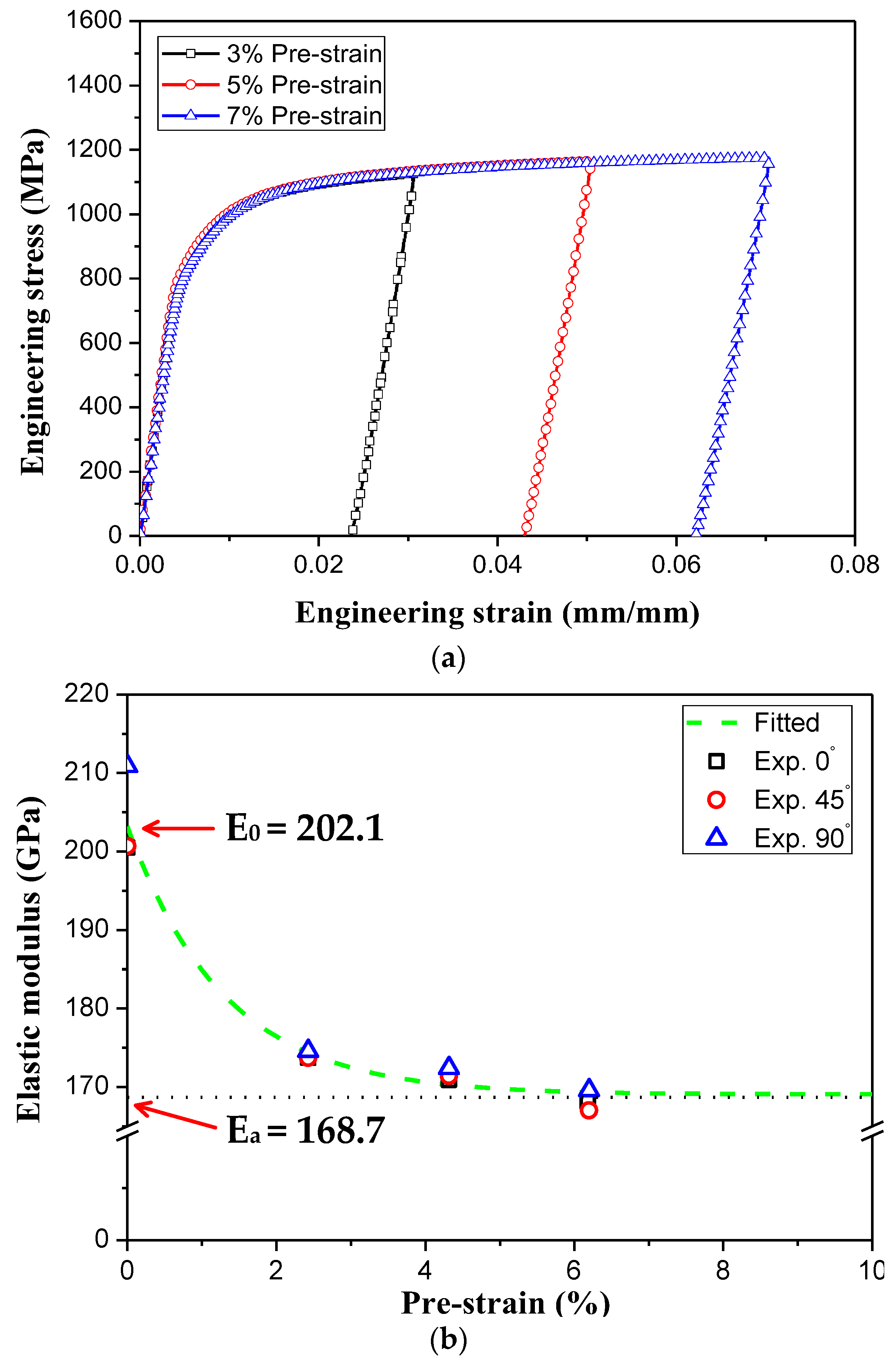
In order to determine the material constants of the chord modulus model, ASTM E8 standard loading–unloading tests were performed on specimens using a MTS universal testing machine for different rolling directions (0°, 45°, 90°). The elastic modulus changes during plastic deformation are reflected in the chord modulus model. The results of this test are shown in Figure 5. Generally, the elastic modulus of steel sheets decreases as the effective strain increases [19,20]. The initial elastic modulus under uniaxial tension, denoted as E0, was determined using the linear regression fitting method. The elastic moduli for pre-strained sheet specimens were defined as the slope of a straight line drawn through the two stress–strain end points at a corresponding prescribed plastic strain. Changes in the chord modulus were applied to the FE simulation along with the hardening model constants. This phenomenon was formulated as shown in Equation (12):
where E represents the unloading elastic model under uniaxial tension, Ea represents the chord modulus obtained under an infinitely large plastic pre-strain, and and are material parameters determining the rate at which E decreases. The optimized constants are given in Table 6.
3. Test Conditions
In this study, FE simulations and experiments were performed for various forming processes including U-bending and T-shape drawing. A commercial program (PamStamp 2G) was used to perform the FE simulation. The experimental and analytical results were compared using various constitutive equations and the material constants determined in Section 2. Both U-bending and T-shape drawing were employed to evaluate the accuracy of springback predictions.
3.1. U-Bending Test
Previous works have confirmed the U-bending test to be a significant verification model for springback prediction [21,22,23]. The tools used in U-bending are shown in Figure 6, consisting of a punch, blank holder, and die. The dimension of the blank was 300.0 mm × 30.0 mm × 1.0 mm. The gap between the die and the punch was designed to be 1.1 mm. Testing was conducted using a 200-ton servo press machine. The total punch stroke was 60.0 mm, with a punch speed of 1 mm/s and a blank holding force of 20 kN. Additional tests were performed in various rolling directions (0°, 45°, 90°). Each set of experimental conditions was repeated five times to ensure the reliability of the experiment. After stamping, the final dimensions of the formed specimens were measured along the middle cross section using a laser coordinate measuring machine (a two-dimensional inspection machine), allowing for comparison between the experimental and FE simulation results.
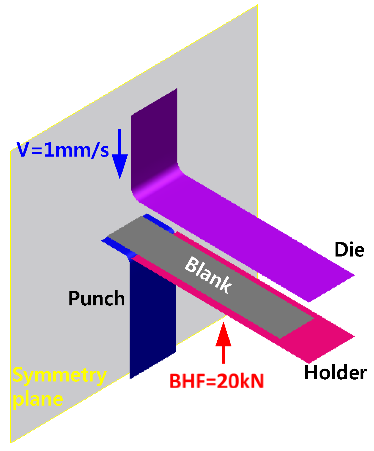
To evaluate the springback behavior observed in the U-bending tests, FE simulations were conducted for forming and springback analysis. The analytical model was designed to mimic the experiment, though only a half model of the tools and blank was simulated as shown in Figure 7, considering the geometric symmetry of the test. The specimen used for FEA was a Belytschko-Lin-Tsay (BLT) shell element of uniform size (1.0 mm × 1.0 mm) with five integration points in the thickness direction. The die was assumed to be a rigid body. The FE simulation conditions were identical to the experimental conditions. The Coulomb friction coefficient between the die and specimen was set to 0.12, a value that assumed an unlubricated condition. In the FE simulation, mass-scaling and mesh-refinement techniques were applied to ensure the efficiency of the analysis. The shapes of the specimens calculated in the FE simulations were compared to those from the experimental results [24].
3.2. T-Shape Drawing Test
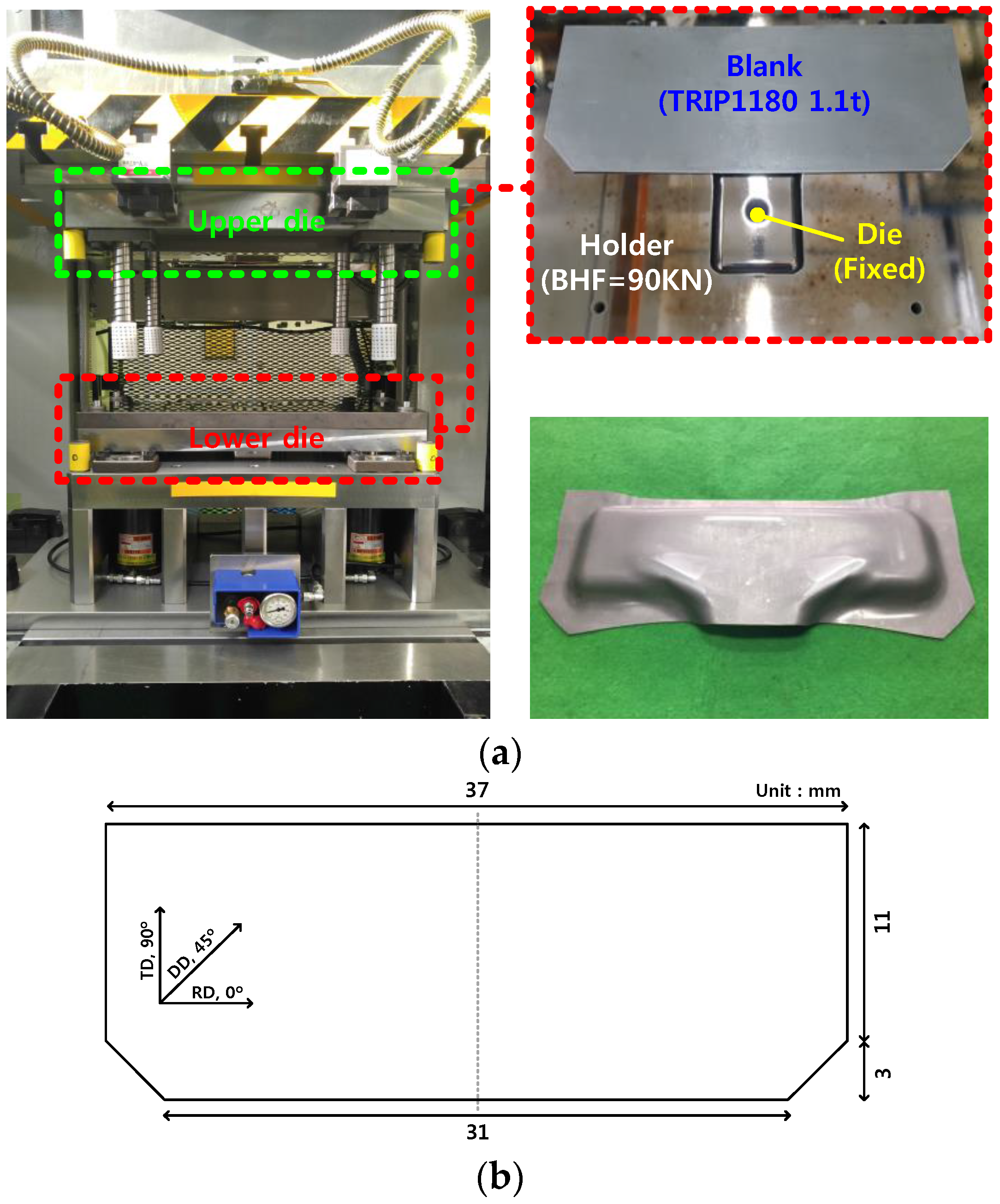
In this study, a T-shape drawing test was performed to evaluate the effect of the constitutive equations on the prediction accuracy of springback in complex deformation modes. The blank size used in T-shape drawing and the experimental set-up for the T-shape drawing test, consisting of a punch, blank holder, and die, are shown in Figure 8. The gap between the die and punch was designed to be 1.1 mm, and the test was conducted using a 200-ton servo press machine. The total punch stroke was 22.0 mm, with a punch speed of 20 mm/s and blank holding force of 90 kN. Experiments were repeated five times to ensure reliability. After stamping, the final dimensions of the formed specimens were measured using a 3D optical scanning system (three-dimensional inspection equipment), allowing for comparison between the experimental and FE simulation results.
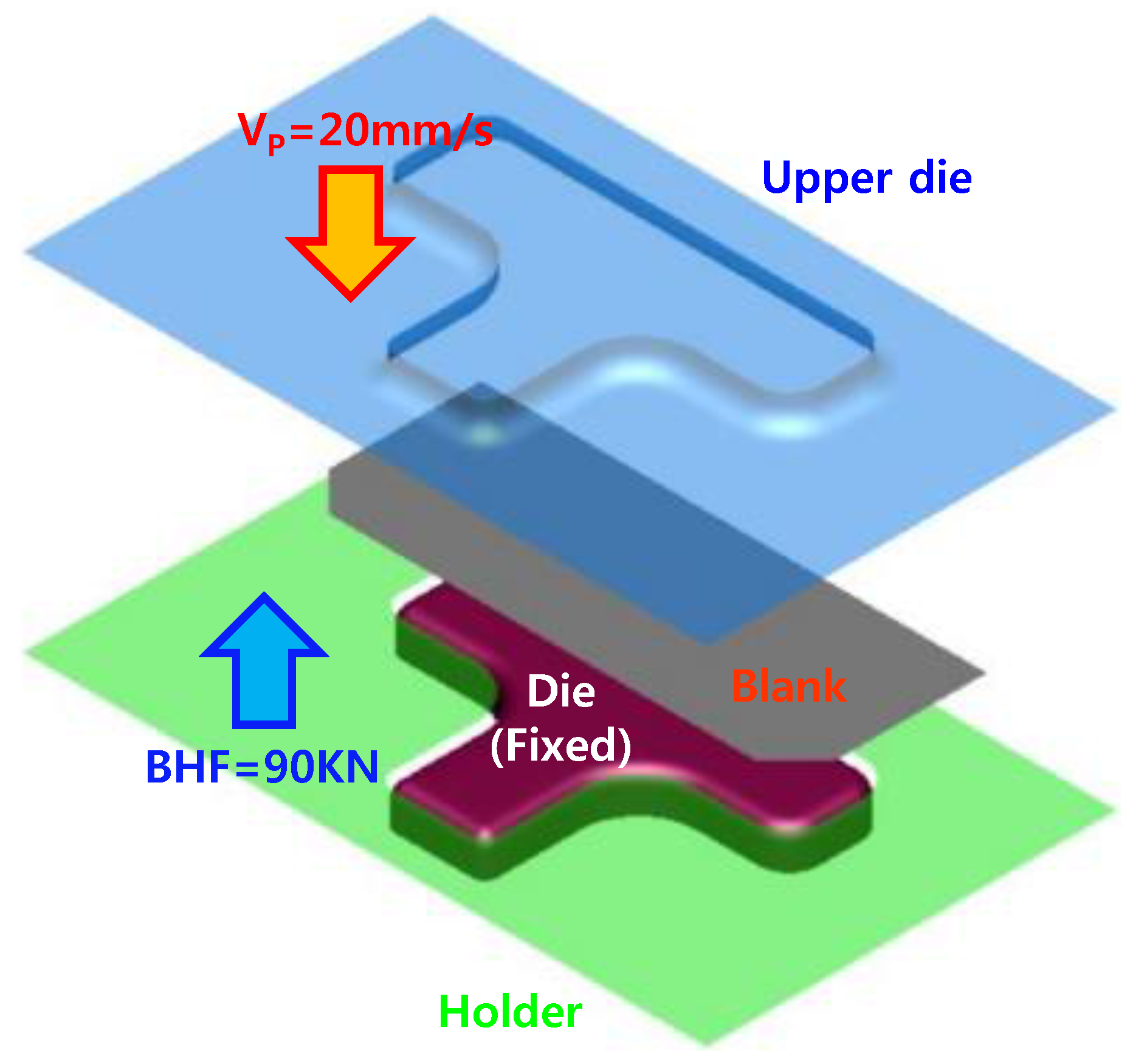
To investigate the springback behavior during T-shape drawing tests, FE simulations were conducted for forming and springback analysis. The analytical model was designed to mimic the experiments, and Figure 9 shows the FE model that was used. A significant number of conditions for the T-shape drawing FE simulation were equivalent to those in the U-bending test simulation and the experimental conditions of the T-shape drawing test. The shapes of the specimens determined via FE simulations were compared with those obtained experimentally. In this study, a commercial reverse-design program (Geomagic Design X), was employed to quantitatively compare the configurations. For this comparison, the experimental results were input as the reference configuration to measure the dimensional errors between the experimental and analytical results.
4. Results and Discussion
4.1. Springback Prediction for U-Bending Test
In order to determine the springback prediction accuracy dependent on the constitutive equations, the predicted U-bending test results were compared to the experimental results. The result is shown in Figure 10. The combination of the Hill’48 yield function and isotropic hardening model resulted in specimen shapes different from those observed experimentally. The combined Yld2000-2d yield function and Yoshida-Uemori model, however, predicted shapes that were similar to those of the manufactured parts.
Springback parameters were employed in this study to quantitatively compare the springback. In Figure 11a, the springback parameters of the defined Numisheet’93 benchmark problem are shown [25]. The 2D draw-bending test proposed as a benchmark problem in Numisheet’93 involves two-dimensional blank holders to show both the effects of the material as well as the process parameters. As previously mentioned, when the results of the combined Yld2000-2d yield function and Yoshida-Uemori model were used, the prediction accuracy for springback was excellent in various rolling directions, including 0°, 45°, and 90°, as shown in Figure 11.
Comparing the predicted and experimental results from the U-bending test, the hardening model was the predominant influence on springback prediction accuracy. When an isotropic hardening model was used, the predicted shape differed significantly from the experimental results. However, when the Yoshida-Uemori model was used, the predicted shape was similar to the experimental results. This demonstrates that the Yoshida–Uemori model resulted in better springback predictions relative to the isotropic hardening model, which is consistent with improved approximations of the reverse-loading curves. For the U-bending test, the deformation mode of the sheet was a uniaxial tension mode, and the sheet was deformed with nonlinear loading conditions. The anisotropic behavior in the uniaxial tension mode could be described well by both the Hill’48 and Yld2000-2d yield functions. However, the hardening behavior from the nonlinear loading conditions is only described by the Yoshida-Uemori model because this model effectively considers changes in the elastic modulus due to pre-strain, the Bauschinger effect, and transient behavior. Furthermore, since the inflow amount of the test specimen was large during the U-bending test, the tension-compression behavior is repeated at the wall of the test specimen as the experiment progresses, as shown in Figure 12. This increases the importance of considering nonlinear loading conditions.
4.2. Springback Prediction for T-Shape Drawing Test
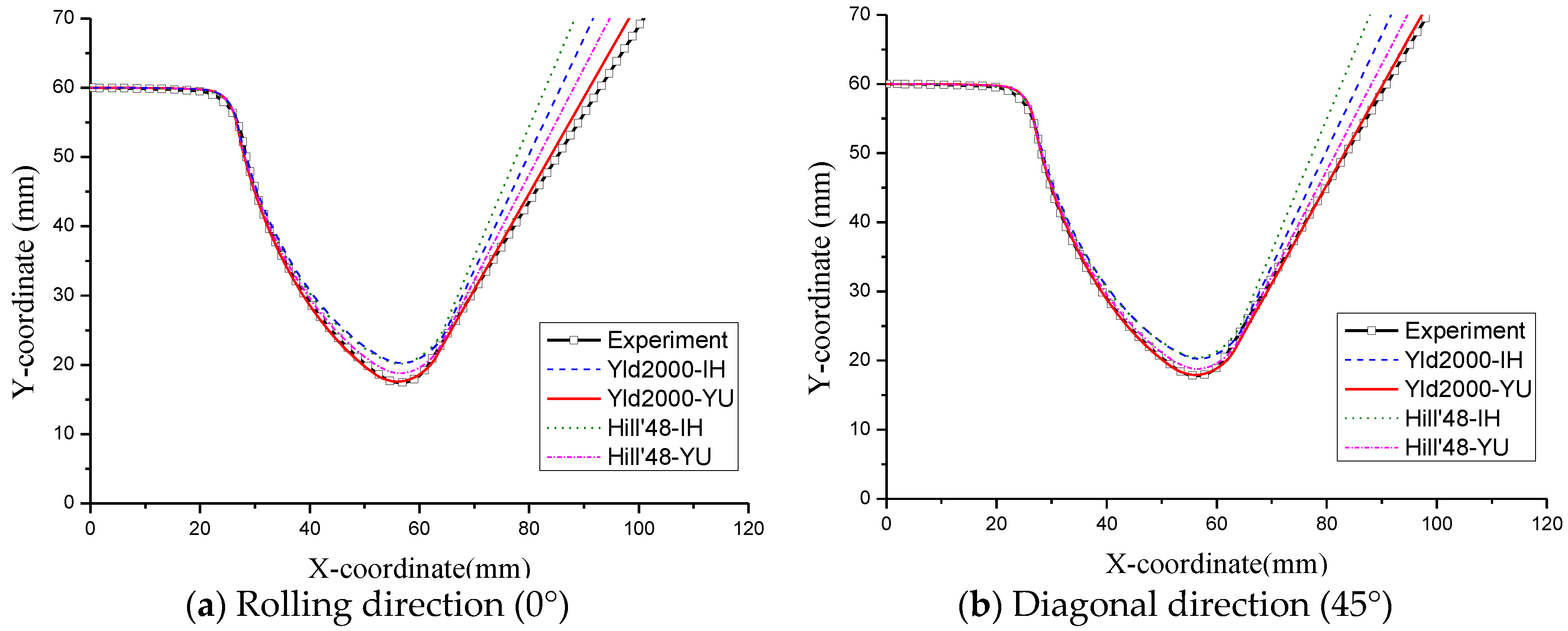
In order to investigate the effects of the constitutive equations on springback prediction accuracy, the predicted and experimental results of the T-shape drawing test were compared, as shown in Figure 13. The springback prediction accuracies in T-shape drawing displayed the same tendencies observed in the U-bending test. The results of the Yld2000-2d yield function and Yoshida-Uemori model combination demonstrated an agreement rate of 82.21%, whereas the combined result of the Hill’48 yield function and isotropic hardening model showed low prediction accuracy with an agreement rate of 73.54%. In this study, the agreement rate was defined as follows:
where A±0.5 represents the area within an allowable tolerance of ±0.5 mm and Atotal represents the total area of the manufactured part. The allowable tolerance was that acceptable variation from the specified dimensions. In this study, the differences between the analytical and experimental results defined using the Geomagic Design X program should be within ±0.5 mm.
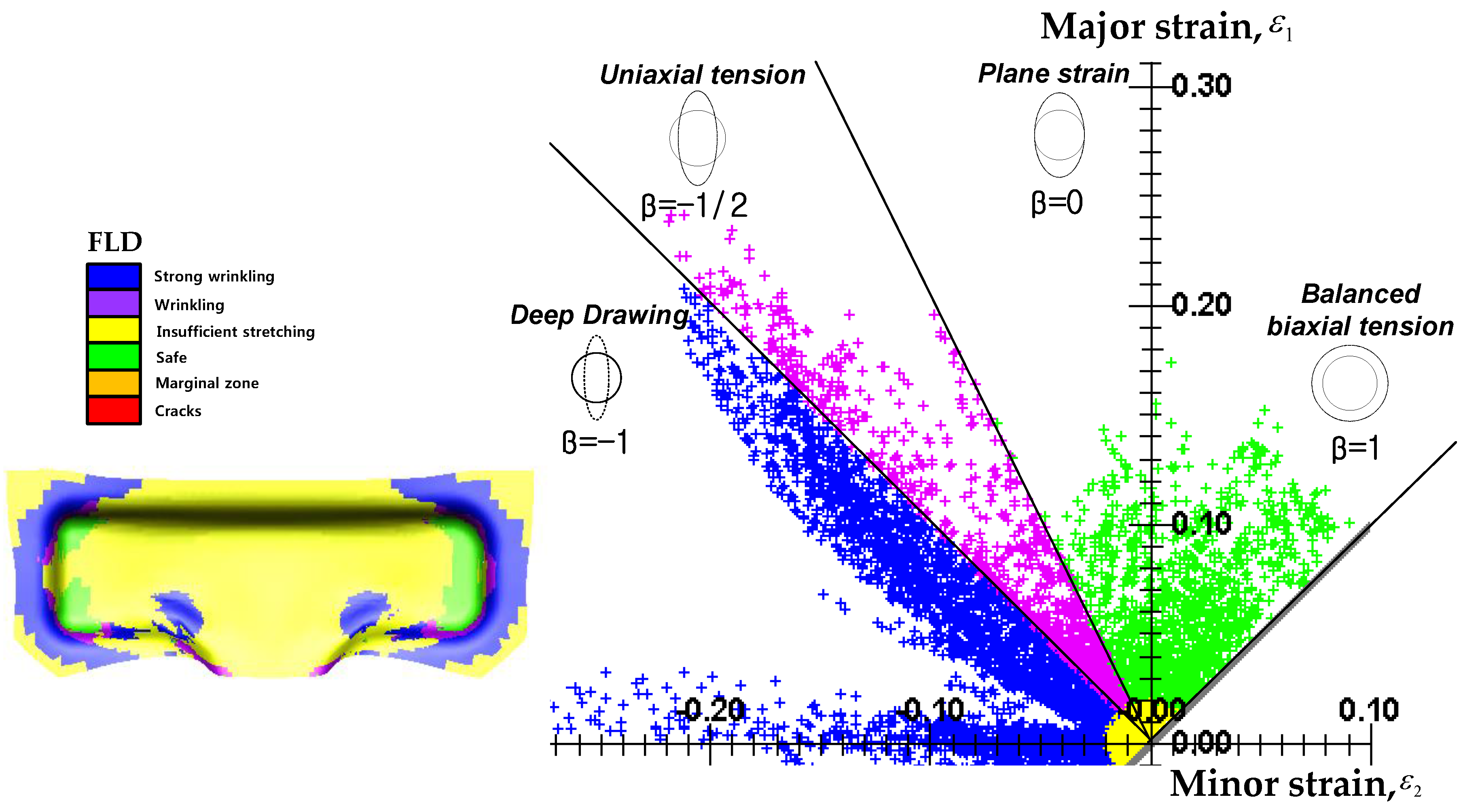
When the predicted and experimental results for the T-shape drawing test were compared, it was observed that the yield function was the predominant influence on springback prediction accuracy. Although the uniaxial deformation mode is dominant in U-bending, T-shape drawing has various deformation modes. Additionally, since the inflow amount of the test specimen is small during the T-shape drawing, it is more important to consider the biaxial Lankford value and yield stress than to consider the non-linear condition. When the Hill’48 yield function was used, the predicted shapes differed greatly from those observed experimentally. However, when Yld2000-2d was used, the predicted shape was similar to the experimental results. In the T-shape drawing test, various deformation modes such as the biaxial tension, plane strain, and deep drawing modes were represented, as shown in Figure 14, and the sheet was deformed with an approximately linear loading condition. The hardening behavior in the linear loading condition could be described well by both the isotropic and Yoshida-Uemori hardening models. However, the yield behaviors for various deformation modes are only described by the Yld2000-2d yield function because it considers Lankford values and yield stresses according to the rolling direction and biaxial deformation mode.
5. Conclusions
In this study, FEA and experiments were conducted to evaluate the effect of constitutive equations on springback prediction accuracy for the cold stamping of a TRIP1180 sheet. Based on the experimental and analytical results, the following conclusions can be drawn:
- Uniaxial tension, bulge, tension-compression, and loading-unloading tests were conducted to investigate anisotropy, nonlinear hardening behavior, and changes in the elastic modulus of a TRIP1180 sheet. The material constants of various constitutive equations were determined based on the experimental results, and were implemented in FE simulations for modeling and analyzing springback.
- FE simulations and experiments were performed to evaluate springback behavior in U-bending and T-shape drawing tests. In both cases, the Yld2000-2d yield function and Yoshida-Uemori model showed excellent prediction accuracy, whereas the Hill’48 yield function and isotropic hardening model showed low prediction accuracy.
- In the U-bending test, the hardening model had a more dominant influence on the prediction accuracy of springback than the yield function due to the nonlinear loading conditions. The hardening behavior observed under nonlinear loading conditions was only described by the Yoshida-Uemori model, because it effectively considered changes in the elastic modulus due to the pre-strain, the Bauschinger effect, and transient behavior.
- In the T-shape drawing test, the yield function had a more dominant influence on the prediction accuracy of springback than the hardening model because various deformation modes were present. The yield behavior for various deformation modes was only described by the Yld2000-2d yield function because this function considered the Lankford values and yield stresses according to the rolling direction and biaxial deformation mode.
- To predict the springback present in AHSS cold stamping, it is necessary to use appropriate constitutive equations according to the forming process. Furthermore, these constitutive equations need to accurately describe the yield behavior, elastic modulus changes, and hardening behavior for a variety of deformation modes.
Acknowledgments
This work was supported by the Small and Medium Business Administration of Korea (SMBA) grant funded by the Korea government (MOTIE) (No. S2315965).
Author Contributions
Ki-Young Seo and Byung-Min Kim conceived and designed the experiments; Ji Hoon Kim interpreted results; Ki-Young Seo and Jae-Hong Kim wrote and revised the manuscript; Hyunk-Seok Lee measured the experiment specimens and supplied the materials.
Conflicts of Interest
The authors declare no conflict of interest.
References
- Hisashi, H.; Nakagawa, T. Recent trends in sheet metals and their formability in manufacturing automotive panels. J. Mater. Process. Technol. 1994, 115, 2–8. [Google Scholar]
- Chen, P.; Koc, M. Simulation of springback variation in forming of advanced high strength steels. J. Mater. Process. Technol. 2007, 190, 189–198. [Google Scholar] [CrossRef]
- Chaboche, J.L. Constitutive equations for cyclic plasticity and cyclic viscoplasticity. Int. J. Plast. 1989, 5, 247–302. [Google Scholar] [CrossRef]
- Lee, M.G.; Chung, K.; Kim, D.; Kim, C.; Wenner, M.L.; Barlat, F. Spring-back evaluation of automotive sheets based on isotropic–kinematic hardening laws and non-quadratic anisotropic yield functions, Part I: Theory and formulation. Int. J. Plast. 2005, 21, 861–882. [Google Scholar]
- Zang, S.L.; Guo, C.; Thuillier, S.; Lee, M.G. A model of one-surface cyclic plasticity and its application to springback prediction. Int. J. Mech. Sci. 2011, 53, 425–435. [Google Scholar] [CrossRef]
- Larsson, R.; Bjoerklund, O.; Nilsson, L.; Simonsson, K. A study of high strength steels undergoing non-linear strain paths—Experiments and modelling. J. Mater. Process. Technol. 2011, 211, 122–132. [Google Scholar] [CrossRef]
- Eggertsen, P.A.; Mattiasson, K. On the modeling of the bending-unbending behaviour for accurate springback predictions. Int. J. Mech. Sci. 2009, 51, 547–563. [Google Scholar] [CrossRef]
- Kim, B.M.; Lee, H.S.; Kim, J.H.; Kang, G.S.; Ko, D.C. Development of Seat Side Frame by Sheet Forming of DP980 with Die Compensation. Int. J. Prec. Eng. Manufacturing. 2017, 18, 115–120. [Google Scholar]
- Yoshida, F. Material models for accurate simulation of sheet metal forming and springback. In Proceedings of the AIP Conference Proceedings 1252, Pohang, Korea, 13–17 June 2010. [Google Scholar]
- Zhu, Y.X.; Liu, Y.L.; Yang, H.; Li, H.P. Development and application of the material constitutive model in springback prediction of cold-bending. Mater. Des. 2012, 42, 245–258. [Google Scholar] [CrossRef]
- Lee, M.G.; Kim, D.; Kim, C.; Wenner, M.L.; Wagoner, R.H.; Chung, K. Spring-back evaluation of automotive sheets based on isotropic-kinematic hardening laws and non-quadratic anisotropic yield functions Part II: Characterization of material properties. Int. J. Plast. 2005, 21, 883–914. [Google Scholar]
- Hill, R. A theory of the yielding and plastic flow of anisotropic metals. Proc. R. Soc. Lond. 1948, 193, 281–297. [Google Scholar] [CrossRef]
- Barlat, F.; Brem, J.C.; Yoon, J.W.; Chung, K.; Dick, R.E.; Lege, D.J.; Pourboghrat, F.; Choi, S.H.; Chu, E. Plane stress yield function for aluminum alloy sheets—Part I: Theory. Int. J. Plast. 2003, 19, 1297–1319. [Google Scholar] [CrossRef]
- SEP1240: Testing and Documentation Guideline for the Experimental Determination of Mechanical Properties of Steel Sheets for CAE-Calculations, 1st ed.; Verlag Stahleisen GmbH: Düsseldorf, Germany, 2006.
- Swift, H.W. Plastic instability under plane stresses. J. Mech. Phys. Solids. 1952, 1, 1–18. [Google Scholar] [CrossRef]
- Yoshida, F.; Uemori, T. A model of large-strain cyclic plasticity describing the bauschinger effect and workhardening stagnation. Int. J. Plast. 2002, 18, 661–686. [Google Scholar] [CrossRef]
- Chongthairungruang, B.; Uthaisangsuk, V.; Suranuntchai, S.; Jiratheranat, S. Springback prediction in sheet metal forming of high strength steels. Mater. Des. 2013, 50, 253–266. [Google Scholar] [CrossRef]
- Nelder, J.A.; Mead, R. A simplex method for function minimization. Comput. J. 1965, 7, 308–313. [Google Scholar] [CrossRef]
- Chatti, S.; Fathallah, R.A. A study of the variations in elastic modulus and its effect on springback prediction. Int. J. Mater. Form. 2014, 7, 19–29. [Google Scholar] [CrossRef]
- Ghaei, A.; Green, D.E.; Aryanpour, A. Springback simulation of advanced high strength steels considering nonlinear elastic unloading–reloading behavior. Mater. Des. 2015, 88, 461–470. [Google Scholar] [CrossRef]
- Lee, M.G.; Kim, D.; Kim, C.; Wenner, M.L.; Wagoner, R.H.; Chung, K. Spring-back evaluation of automotive sheets based on isotropic-kinematic hardening laws and non-quadratic anisotropic yield functions, Part III: Applications. Int. J. Plast. 2005, 21, 915–953. [Google Scholar] [CrossRef]
- Ouakdi, E.H.; Louahdi, R.; Khirani, D.; Tabourot, L. Evaluation of springback under the effect of holding force and die radius in a stretch bending test. Mater. Des. 2012, 35, 106–112. [Google Scholar] [CrossRef]
- Jung, J.B.; Jun, S.W.; Lee, H.S.; Kim, B.M.; Lee, M.G.; Kim, J.H. Anisotropic hardening behaviour and and springback of advanced high-strength steels. Metals 2017, 7, 480. [Google Scholar] [CrossRef]
- Gomes, C.; Onipede, O.; Lovell, M. Investigation of springback in high strength anisotropic steels. J. Mater. Process. Technol. 2005, 159, 91–98. [Google Scholar] [CrossRef]
- Makinouchi, A.; Nakamachi, E.; Onate, E.; Wagoner, R.H. NUMISHEET’93 Benchmark Problem. In Proceedings of the 2nd International Conference on Numerical Simulation of 3D Sheet Metal Forming Processes-Verification of Simulation with Experiment, Isehara, Japan, 31 August–2 September 1993. [Google Scholar]
Figure 1.
Results of uniaxial tension and bulge tests.

Figure 2.
Yield surfaces characterized by different yield functions.
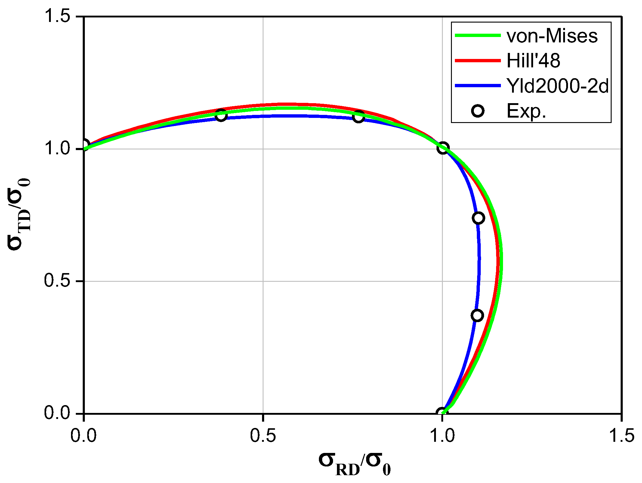
Figure 3.
(a) Dimensions of the specimen used for tension–compression test. (b) A schematic view of the tension-compression test.
Figure 3.
(a) Dimensions of the specimen used for tension–compression test. (b) A schematic view of the tension-compression test.
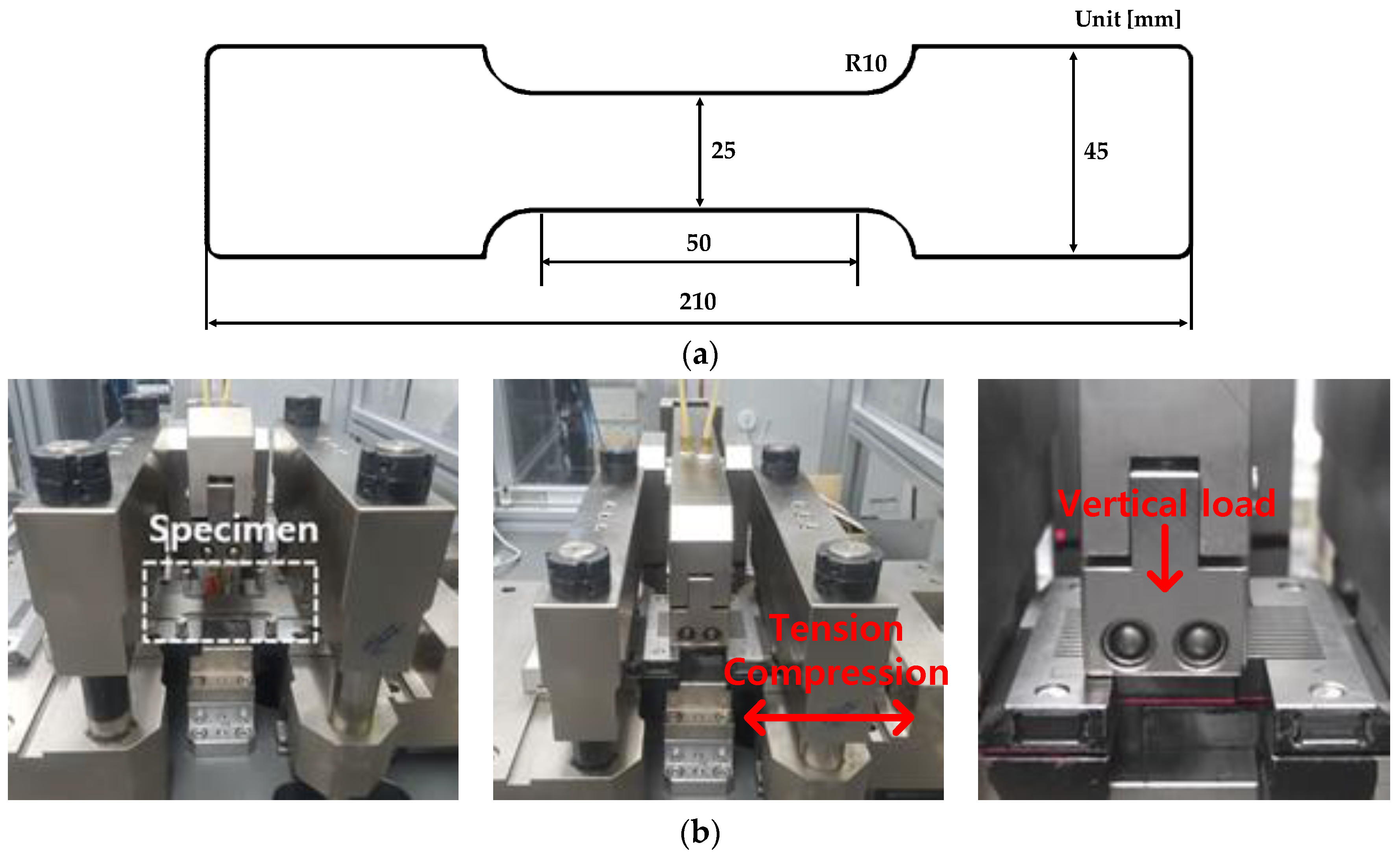
Figure 4.
Measured and calculated tension-compression stress-strain curves from multiple hardening models.
Figure 4.
Measured and calculated tension-compression stress-strain curves from multiple hardening models.
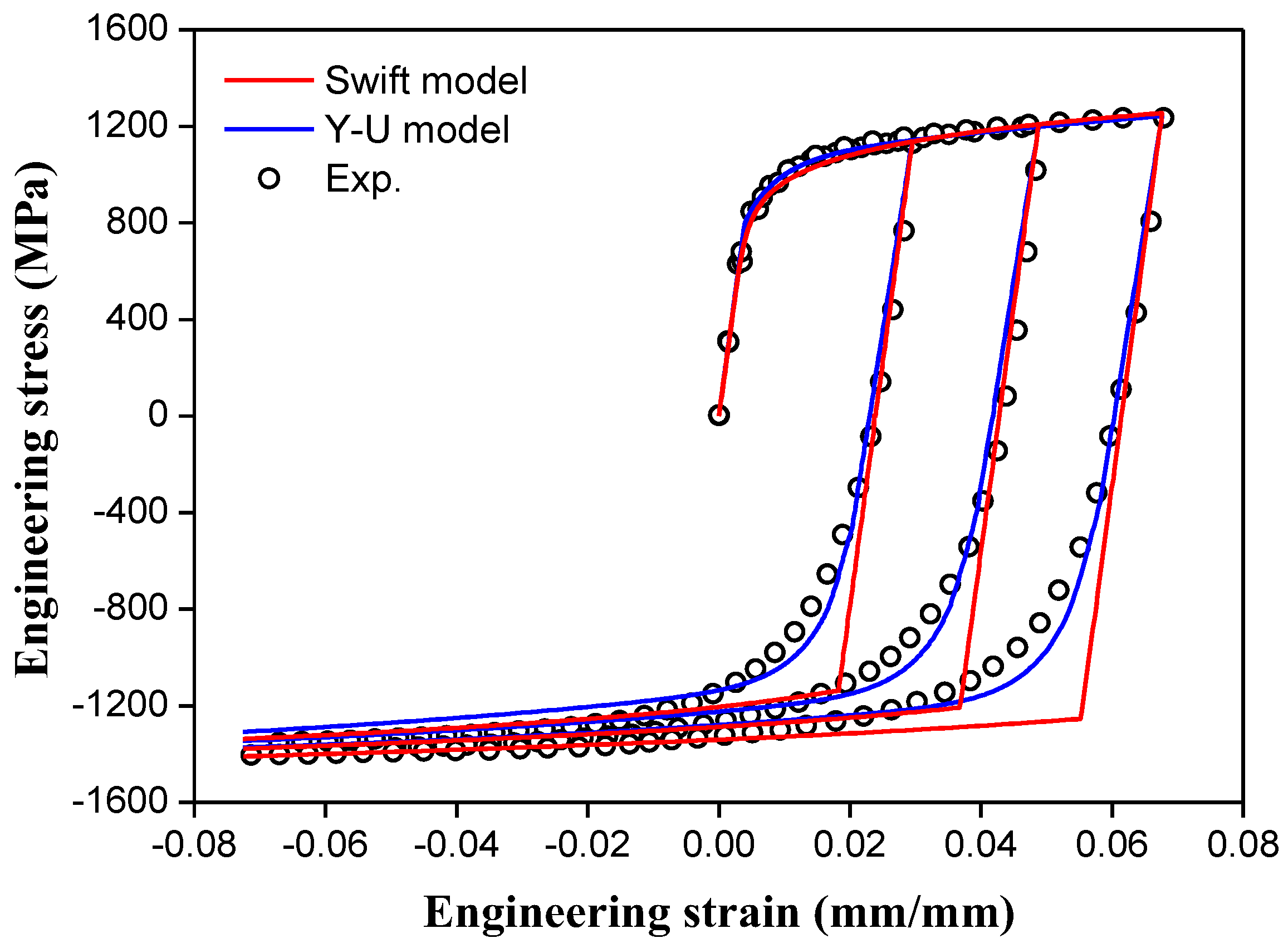
Figure 5.
(a) Results of loading-unloading test. (b) Results of chord modulus model.

Figure 6.
(a) Tools for U-bending test. (b) Blank size of U-bending test.
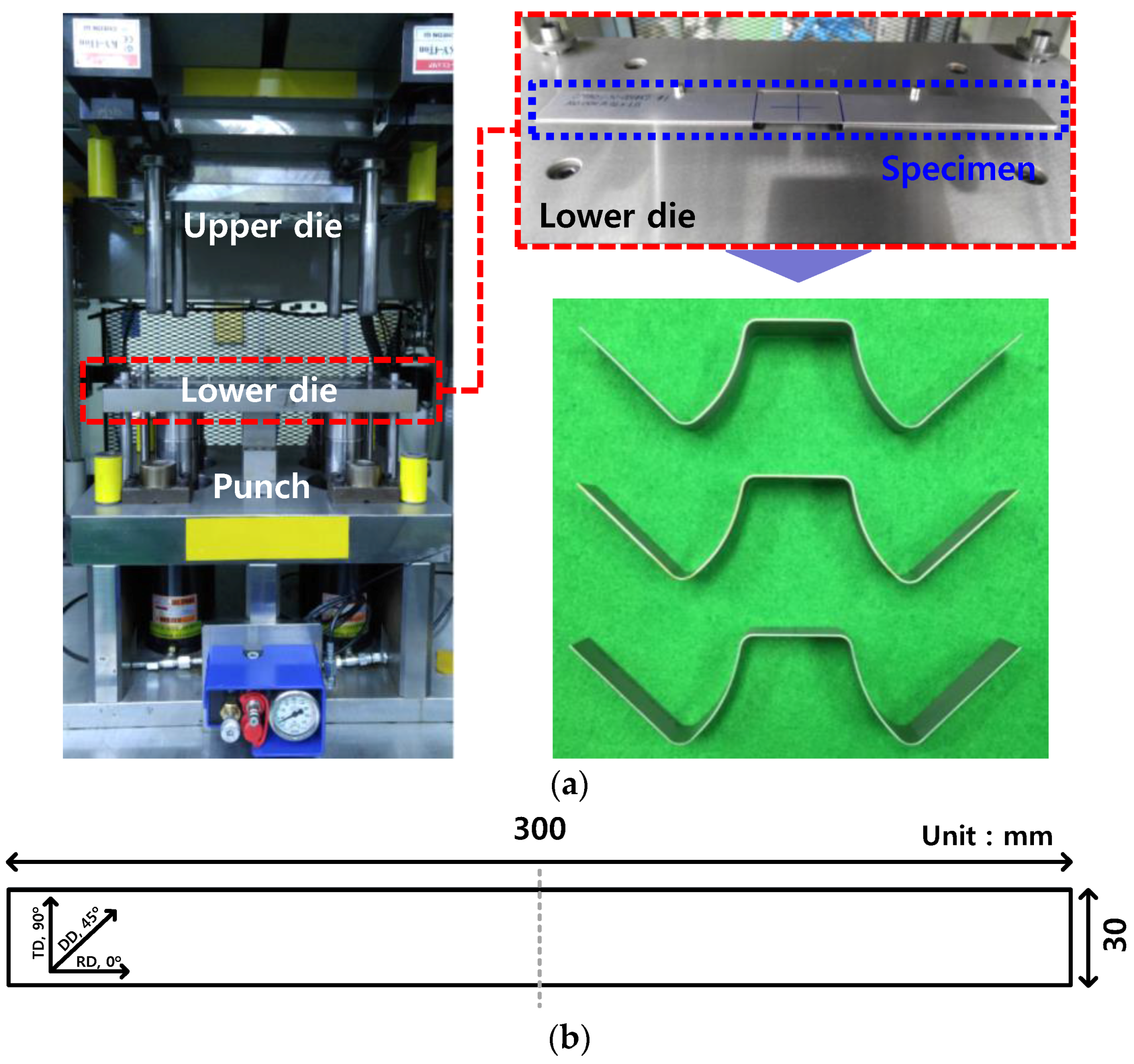
Figure 7.
Finite element (FE) model of U-bending.

Figure 8.
(a) Experimental set-up for T-shape drawing test. (b) Blank size of T-shape drawing test.

Figure 9.
Finite element (FE) model for T-shape drawing test.

Figure 10.
Shape comparison between predictions and experiments for U-bending test.

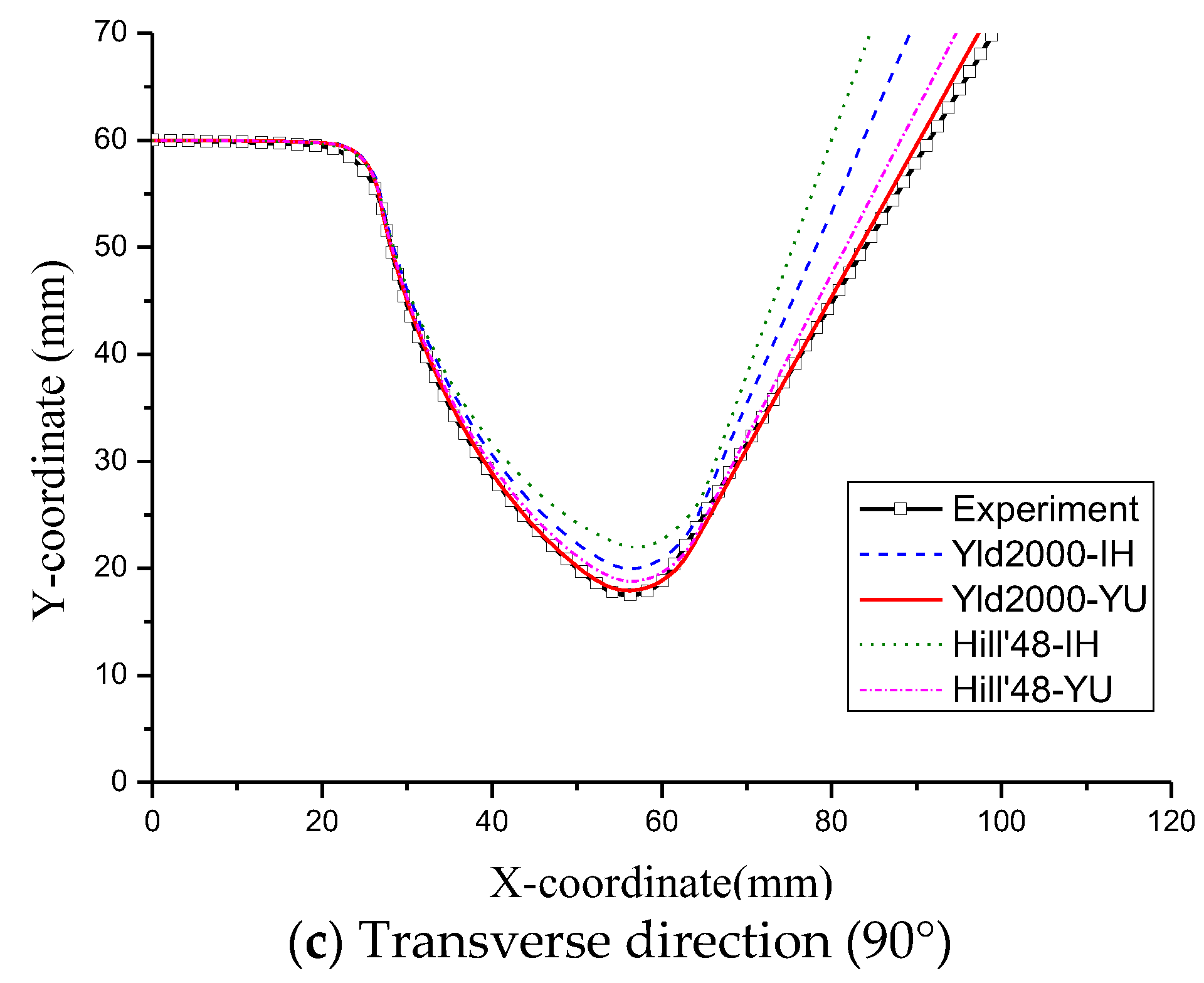
Figure 11.
Comparison of springback with springback parameters for U-bending test.
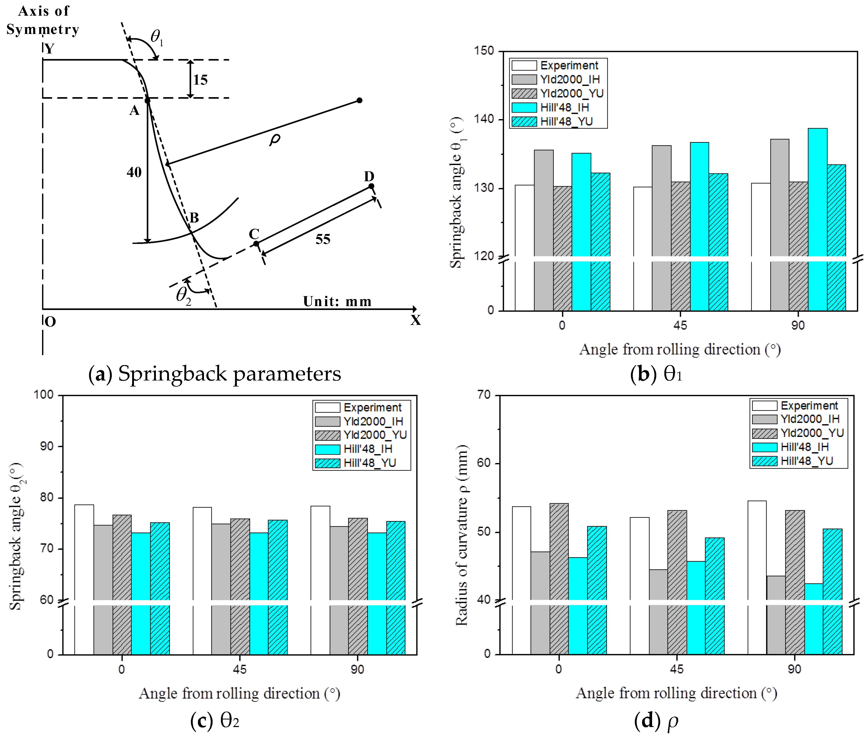
Figure 12.
Tension-compression behavior of the U-bending test.
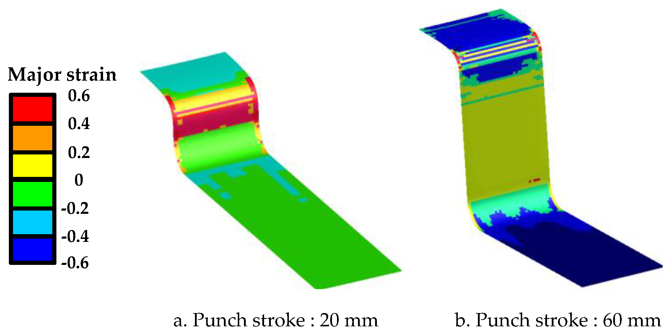
Figure 13.
Comparison between predictions and experiments for T-shape drawing test.
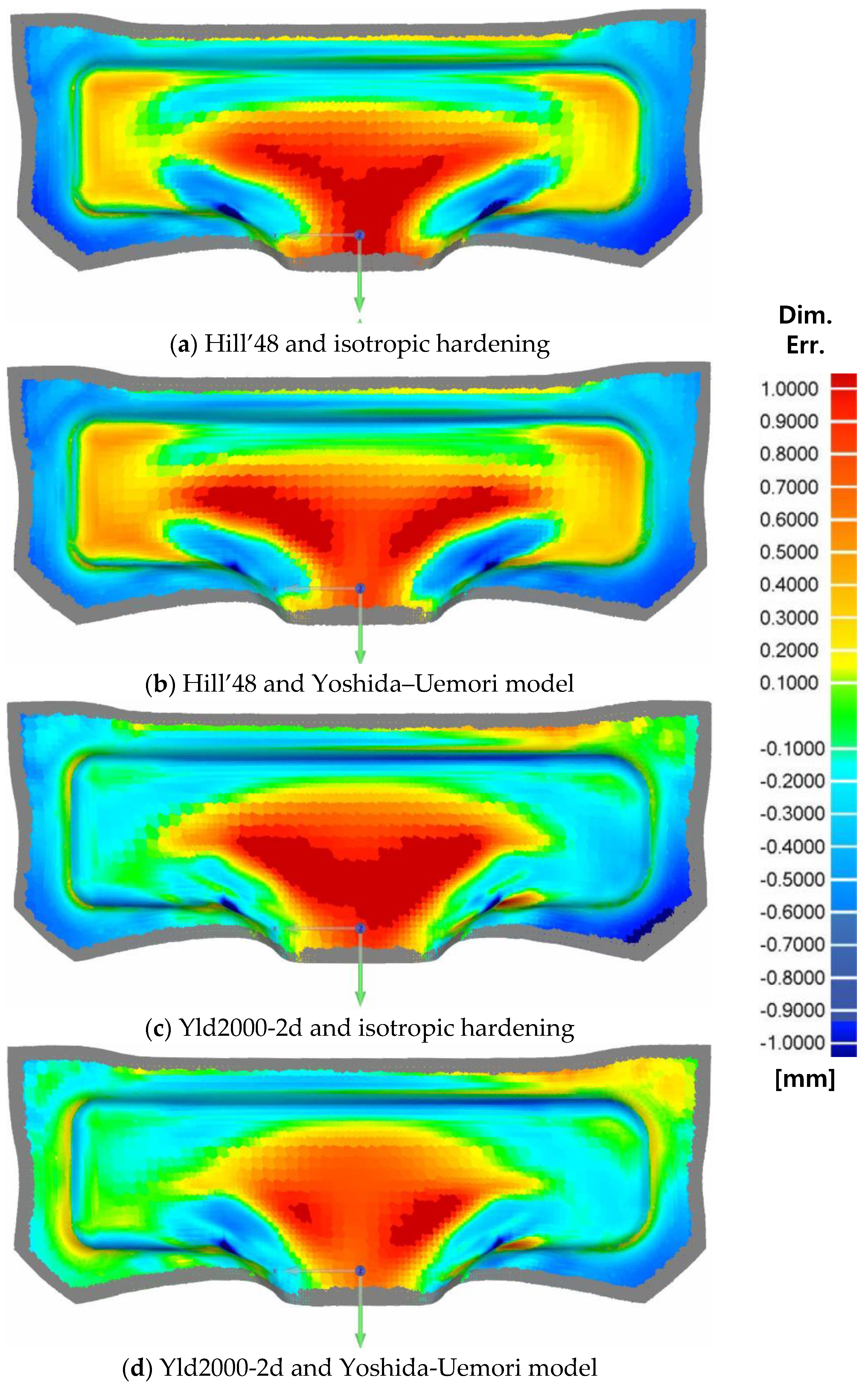
Figure 14.
T-shape drawing with various deformation modes.

Table 1.
Material properties of TRIP1180 steel.
| Test Direction | E0 (GPa) | YS (MPa) | UTS (MPa) | Elongation (%) | R-Value |
|---|---|---|---|---|---|
| Rolling direction (0°) | 200.5 | 861.9 | 1180 | 17.2 | 0.795 |
| Diagonal direction (45°) | 200.7 | 866.6 | 1175 | 16.0 | 0.958 |
| Transverse direction (90°) | 206.3 | 866.2 | 1182 | 14.9 | 0.967 |
Table 2.
Material constants of TRIP1180 for the Hill’48 yield function.
| Material | F | G | H | N |
|---|---|---|---|---|
| TRIP1180 | 0.4580 | 0.5571 | 0.4429 | 1.480 |
Table 3.
Material constants of TRIP1180 using the Yld2000-2d yield function.
| α1 | α2 | α3 | α4 | α5 | α6 | α7 | α8 |
|---|---|---|---|---|---|---|---|
| 0.9471 | 1.0199 | 0.9867 | 0.9925 | 1.0141 | 0.9815 | 0.9910 | 1.0007 |
Table 4.
Coefficients of the Swift isotropic hardening model for TRIP1180.
| Material | K (MPa) | n | |
|---|---|---|---|
| TRIP1180 | 1672.8 | 0.1044 | 4.8605E-14 |
Table 5.
Material constants of TRIP1180 for the Yld2000-2d yield function.
| Y | B | Rsat | b | m | C1 | C2 | εp,ref |
|---|---|---|---|---|---|---|---|
| 800 | 284.9 | 294.2 | 88 | 9.62 | 366.8 | 366.8 | 0.005 |
Table 6.
Material constants of TRIP1180 softening behavior.
| Material | E0 (GPa) | Ea (GPa) | ξ |
|---|---|---|---|
| TRIP1180 | 202.1 | 168.7 | 72.9 |
© 2017 by the authors. Licensee MDPI, Basel, Switzerland. This article is an open access article distributed under the terms and conditions of the Creative Commons Attribution (CC BY) license (http://creativecommons.org/licenses/by/4.0/).
Share and Cite
MDPI and ACS Style
Seo, K.-Y.; Kim, J.-H.; Lee, H.-S.; Kim, J.H.; Kim, B.-M. Effect of Constitutive Equations on Springback Prediction Accuracy in the TRIP1180 Cold Stamping. Metals 2018, 8, 18. https://doi.org/10.3390/met8010018
AMA Style
Seo K-Y, Kim J-H, Lee H-S, Kim JH, Kim B-M. Effect of Constitutive Equations on Springback Prediction Accuracy in the TRIP1180 Cold Stamping. Metals. 2018; 8(1):18. https://doi.org/10.3390/met8010018
Chicago/Turabian StyleSeo, Ki-Young, Jae-Hong Kim, Hyun-Seok Lee, Ji Hoon Kim, and Byung-Min Kim. 2018. "Effect of Constitutive Equations on Springback Prediction Accuracy in the TRIP1180 Cold Stamping" Metals 8, no. 1: 18. https://doi.org/10.3390/met8010018
Note that from the first issue of 2016, this journal uses article numbers instead of page numbers. See further details here.