Development of Amplifier Circuit by Active-Dummy Method for Atmospheric Corrosion Monitoring in Steel Based on Strain Measurement


1
Department of Risk Management and Environmental Sciences, Graduate School of Environmental and Information Sciences, Yokohama National University, Yokohama 240-8501, Japan
2
Department of Electrical Engineering, Faculty of Engineering, Lampung University, Bandar Lampung 35141, Indonesia
3
Division of Material Science and Engineering, Graduate School of Engineering, Yokohama National University, Yokohama 240-8501, Japan
4
Nippon Steel & Sumikin Research Institute, Tokyo 100-0005, Japan
*
Author to whom correspondence should be addressed.
Metals 2018, 8(1), 5; https://doi.org/10.3390/met8010005
Submission received: 31 October 2017
/
Revised: 14 December 2017
/
Accepted: 18 December 2017
/
Published: 22 December 2017
(This article belongs to the Special Issue Advanced Non-Destructive Testing in Steels)
Abstract
:This paper describes an amplifier circuit fabricated by the active-dummy method for atmospheric corrosion monitoring based on strain measurement. The circuit was used to determine the relationship between the voltage and strain. Experiments involving the thickness reduction of low-carbon steel test pieces induced by galvanostatic electrolysis were carried out with the amplifier circuit. The circuit was capable of accurately measuring signals induced by the thickness reduction of the test piece. Moreover, the circuit was assessed for the effects of environmental temperature drift, and was found to exhibit a high tolerance. The proposed amplifier circuit would be suitable for atmospheric corrosion monitoring in many types of infrastructure.
1. Introduction
Corrosion damages the steel that is used for many types of infrastructure. It causes significant damage to steel, which can lead to catastrophic structural failure. Based on this, corrosion detection on steel structures is necessary. There is a great deal of research on how to detect corrosion, such as using a radio-frequency identification (RFID) sensor [1,2,3] and the methods involving optic fibers [4,5,6,7,8]. These methods are all effective in ensuring the safety level of steel structures.
Atmospheric corrosion monitoring is also important in predicting the corrosion damage of steel structures. Factors governing atmospheric corrosion are the temperature, dew, precipitation, relative humidity, and nitrate, chloride, and sulfate ions. At high temperatures, some electrolytes become highly reactive. Dew, precipitation, and relative humidity also have a large effect on the corrosion process. Nitrate, chloride, and sulfate ions can increase the corrosiveness of the environment. All these factors require further elaboration in order to clearly describe the phenomenon of atmospheric corrosion.
Several conventional methods for atmospheric corrosion monitoring, such as weight and thickness loss [9,10,11,12,13,14,15,16], polarization resistance [17], the corrosion behavior of steels with different nickel content [18,19], stainless steels [20], galvanized steel [21,22], zinc [23], and electrochemical impedance spectroscopy [24,25,26,27,28,29], have been extensively used to monitor atmospheric corrosion. Recent developments for monitoring atmospheric corrosion including using electric resistance sensors [30,31], pulsed Eddy current testing (ECT) [32], and passive wireless sensors [33]. In addition to new methods, in order to develop the atmospheric corrosion monitoring (ACM) sensor, many researchers also investigated various characteristics of corrosion. These included metal loss, material characteristics of corrosion layers [34] which were analyzed using different analysis methods, such as finite element analysis (FEA) models that used two layers of the corrosion layer and test piece [7,30], microscopic analysis [5,28], and X-ray diffraction [6,25,26]. In addition to these techniques, electrochemical methods are useful because they allow in situ corrosion monitoring [35]. However, precise monitoring is difficult because electrochemical methods are very sensitive to the corrosion reactions. Once an electrode begins to corrode, the redox reactions of the corrosion products affect the current density signals. In the case of steel, ferrous and ferric ions coexist in the corrosion product. These factors ultimately prevent precise evaluation of atmospheric corrosion. Thus, a highly-accurate in situ sensor capable of monitoring atmospheric corrosion is needed.
Against this background, we have developed a new principle for measuring corrosion rates in real-time. A highly-accurate in situ sensor, capable of atmospheric corrosion monitoring by measuring the thickness of carbon steel, is proposed. Previous research on in situ monitoring of thinning of test pieces by galvanostatic electrolysis [36] has shown that strain can provide a measure of the reduction in thickness due to corrosion. However, in actual applications, there is significant noise due to variations in temperature and other factors during field measurements.
Therefore, the purpose of this study is to develop an amplifier circuit for atmospheric corrosion monitoring based on strain measurement by using the active-dummy method, which has high sensitivity and can reduce the effect of temperature on the measurement environment. A dummy circuit compensated for the temperature drift in the signal with an active circuit was successfully designed, and experiments involving galvanostatic electrolysis were conducted by using the amplifier circuits to determine the thinning of test pieces through strain measurements. In addition, the effect of the temperature on the measurement environment on the signals, was investigated.
2. Materials and Methods
2.1. Design of Amplifier Circuit by Active-Dummy Method
2.1.1. Principle of ACM (Atmospheric Corrosion Monitoring) Sensor Based on Strain Measurement
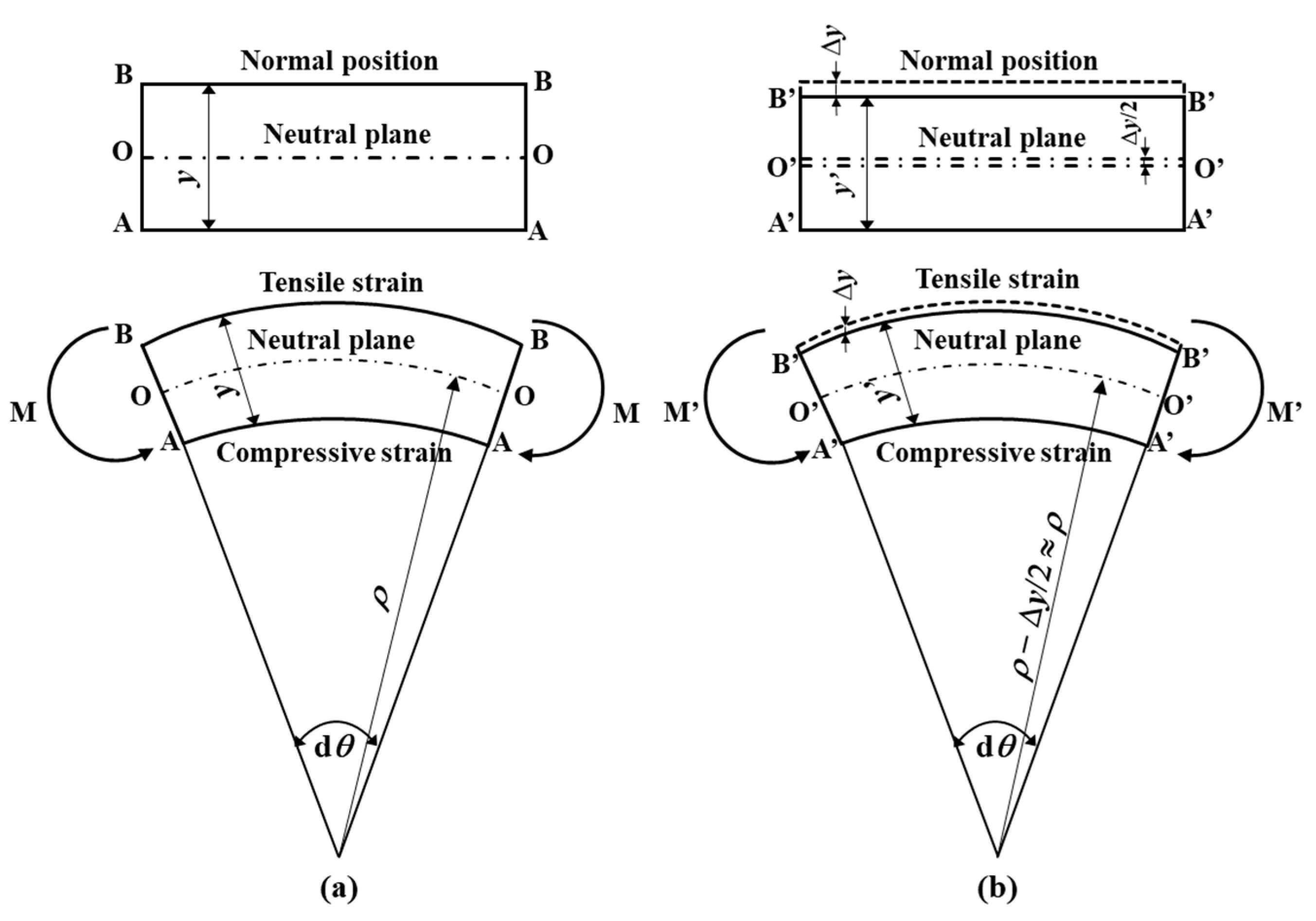
The mechanism whereby the ACM sensor can measure the thinning of test pieces is shown in Figure 1. A test piece with a thickness y is subjected to a bending moment M; the radius of the curvature of the test piece is denoted by ρ, and the center angle by dθ. Line segment O-O represents the neutral plane, and its length is the unaltered by the deformation. Line segment A-A is shortened upon deformation and its length is equal to (ρ − ) dθ. The strain on the A-A surface can be expressed by [35]:
When the test piece thickness is reduced as a result of corrosion, the distance between the neutral plane and the surface of the test piece decreases, as seen in Figure 1. From Equation (1), the change in strain is expressible as:
The change in the test piece thickness under a constant ρ can be measured by the change in strain of the concave surface. Through Equation (2), we can monitor the diminishing thickness of the test piece by monitoring the change in strain.
2.1.2. Concept of Amplifier Circuit by Active-Dummy Method
The amplifier circuit fabricated by the active-dummy method for atmospheric corrosion monitoring consists of bridge circuits with strain gauge sensors connected to the test piece, pre-amplifier circuits based on an instrumentation stage operational amplifier with a circuit identical to that used in the active-dummy method, and a differential circuit that differs from the active-dummy circuit. The design concept of the amplifier circuit used in the active-dummy method to monitor atmospheric corrosion is illustrated in Figure 2. εμ,τ,ο is the strain with input from the signal and environmental factor. εμ is the strain from the thinning of the test piece due to corrosion stress. ετ,ο is the strain due to environmental effects, such as temperature and humidity. The active circuit has not only εμ but also ετ,o as inputs, whereas in the case of the dummy circuit, the only input is ετ,ο. The differential circuit subtracts the output from the active circuit from the output from the dummy circuit. Since the dummy circuit compensates for the effects of environmental or atmospheric conditions on the active circuit, an accurate value is obtained for εm.
2.2. Experimental Setup
2.2.1. Design of ACM Sensor
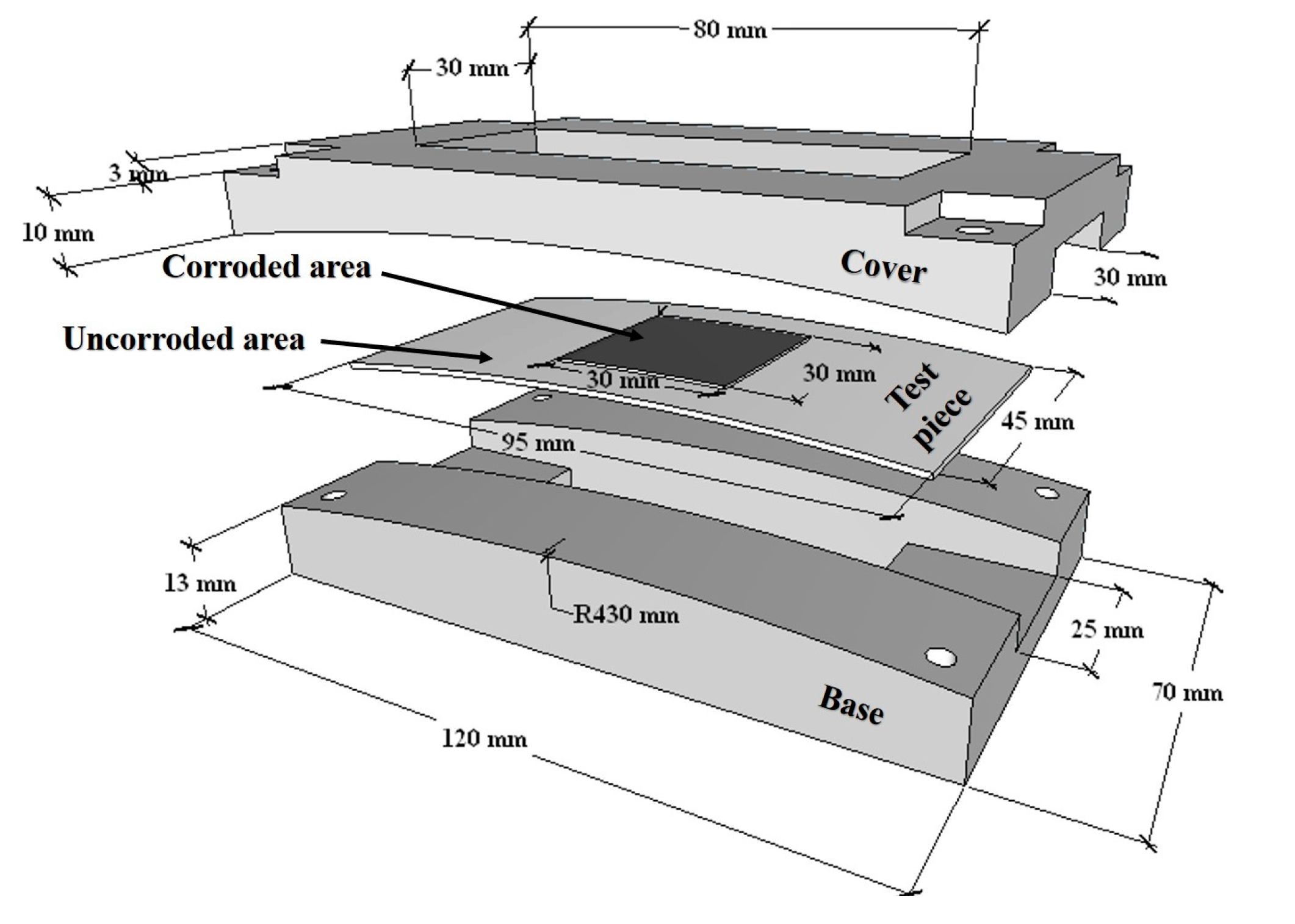
The test piece was 95 mm in length, 45 mm in width, 0.48 mm in thickness, and made of low-carbon steel. To remove the residual stress, the test piece was heat-treated at 450 °C for 1 h. A corroded area, 30 mm in length and 30 mm in width, was arranged in the center of the test piece with no plastic coating, while the remaining area was coated with plastic to prevent corrosion (in other words, an uncorroded area), as shown in Figure 3. The corroded area which becomes thinner as a result of corrosion, enables the calculation of the reduction in thickness. To calculate the radius of the curvature of the apparatus, ρ, Hooke’s law and Equation (1) can be combined, yielding the equation:
By using a yield stress of 240 MPa, a Young’s modulus of 210 GPa [34], and a test piece thickness of 0.5 mm, ρ in the elastic deformation range was calculated via Equation (3) to be 219 mm. To prevent local plastic deformation of the test piece, ρ should be roughly twice this value. Thus, ρ = 430 mm.
The apparatus comprises a base and cover made of polyvinyl chloride, as shown in Figure 3. According to [34], Δy = 0.86 × Δε. The units of Δε are με (µm/m), the units of Δy are μm, and the units of the coefficient 0.86 are m/ε. A strain gauge, which was in contact with the back of the test piece, was installed in the apparatus.
2.2.2. Strain Gauge Configuration of Test Piece for Active and Dummy Circuit
The test piece for the active circuit is TPA, and the test piece for the dummy circuit is TPD. TPA has active and dummy strain gauges at positions 1 and 3, and a strain gauge for the commercial strain measurement device at position 1. TPD has active and dummy strain gauges at positions 2 and 3. TPA has a 900 mm2 corroded area at the center of the test piece; the remaining area is uncorroded. TPD only has a corroded area. The configuration of the strain gauges on the test piece is shown in Figure 4. Position 1 is at the center of the active test piece with curvature ρ, and has active gauges (RAA) on the back of the corrosion area. Position 2 is at the center of the dummy test piece with curvature ρ, and has active gauges (RAD) on the back of the uncorroded area. Position 3 is at the edge of both test pieces on the back of the uncorroded area, and has dummy strain gauges (RDA and RDD). The first letter in the subscript denotes whether the gauge is active or dummy, while the second letter denotes whether the circuit is active or dummy. RAA is placed at the center of TPA with curvature ρ to exert a stress on the strain gauges, as well as on the back of the corroded area in order to receive signals from the corrosion-induced thinning of the test piece. RDA is placed at the edge of TPA and on the back of the corroded area without stress to compensate for the effects of atmospheric conditions on the active gauge. RAD and RDD, as identical gauges of the active circuit, compensated for the active circuit and are placed in the uncorroded area on TPD. SG is the strain gauge for measuring the strain in the corroded area with a commercial strain meter and is placed at the center of the corroded area without bending. The strain gauges and their functions are shown in Table 1.
2.2.3. Design of the Amplifier Circuit with the Active-Dummy Method
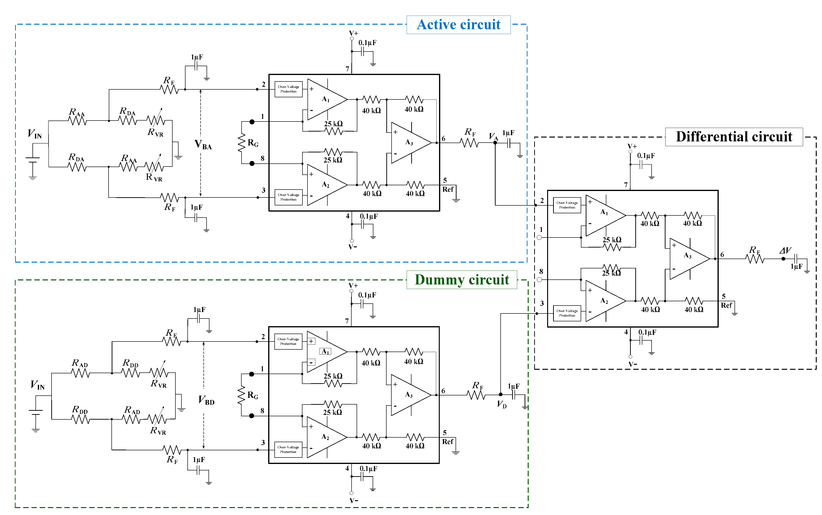
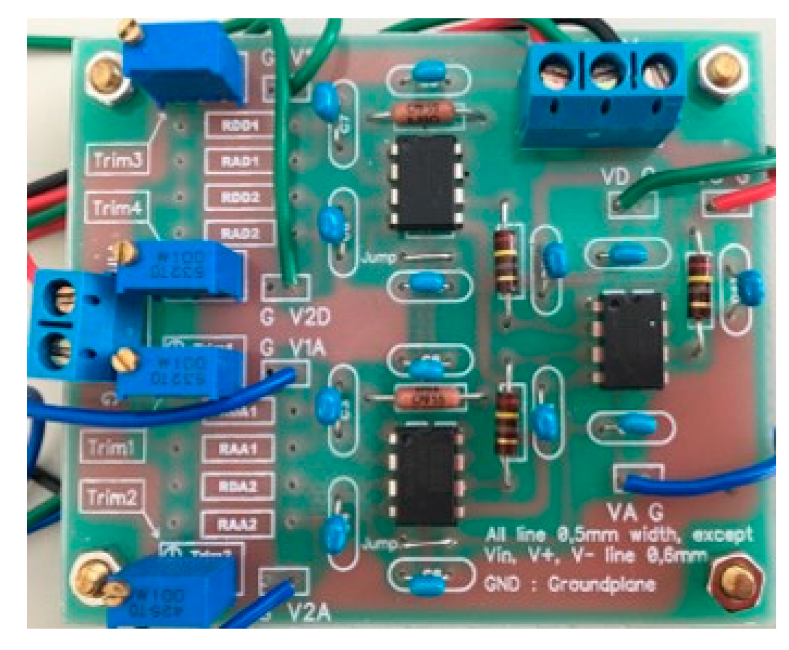
The amplifier circuit used in the active-dummy method (see Figure 5), with its gain of 10,000, was designed to measure very small strains of Tokyo Sokki FLA-5-11 strain gauges (Tokyo Sokki Kenkyujo Co., Ltd., Tokyo, Japan) when it was placed in a bridge circuit, such that RAA, RDA, RAD and RDD, all have the same resistance of 120 Ω. Using a voltage input (VIN) of 3 V to adjust the current through the strain gauge, the output voltages of (i) the active bridge circuit, VBA, (ii) the dummy bridge circuit, VBD, (iii) the active circuit, VA, (iv) the dummy circuit, VD, and (v) the amplifier circuit, ΔV, should all be zero under balanced conditions. When a variation in the strain gauge resistance appeared in the signal, VBA appeared and, when amplified, became VA, in addition to ΔV also appearing. The input for the operational amplifier VCC and VEE is 10 V and became the maximum voltage of the circuit. To reduce the noise, capacitors were used as a filters in the input area, as well as a filter consisting of capacitors and resistors in the output area. INA128 op-amplifiers (Texas Instruments, Dallas, TX, USA), which are largely unaffected by temperature variations, were used. The other components had low coefficients of thermal expansion and low tolerance. Figure 6 illustrates an amplifier circuit built by the present active-dummy method.
2.2.4. Master Curve of the Strain-Voltage Relationship
This experiment employed a Graphtec GL7000 data logger (Graphtec Co., Yokohama, Japan) to monitor the voltage from the amplifier circuit and the temperature of the measurement environment, and a Kyowa Sensor Interface PCD-300B (Kyowa Electronic Instruments Co., Ltd., Tokyo, Japan) to measure the strain.
To induce a strain on TPA, the edge of the test piece was fixed, and different weights were attached to the edge of the test piece. The center of the test piece exhibited a strain due to bending. Within the elastic strain region of the test piece, the relationship between strain and weight was linear. Meanwhile, the TPD did not detect the variations in strain, only the behavior of the environment.
The output voltages of the active circuit, dummy circuit, and amplifier circuit were measured by taking data at a rate of 1 sample/s. SG, which has the same position as RAA, was modified from the cantilever position using a balance. SG, VA, and VS change simultaneously as the balance is moved. The balance was modified every 50 g to get the variation in the data up to the 10 V maximum.
2.2.5. In Monitoring of Thinning of Test Piece by Galvanostatic Electrolysis
This experiment was carried out to investigate the accuracy of the amplifier circuit using the active-dummy method, as described in Section 2.1.2. Figure 7 shows the experimental setup used to measure the change in strain due to the thinning of the TPA of the ACM sensor through galvanostatic electrolysis. The electrolytic solution in the reservoir was 1 mol·L−1 hydrochloric acid solution. The working electrode was TPA, and the counter electrode consisted of the same material as TPA. The thickness of the working electrode was reduced by galvanostatic electrolysis with a current of 1 A, and the strain of the test piece was measured to assess the change in thickness. The corroded area was 900 mm2. The difference in weight (ΔW) and thickness (ΔyA) of the test piece of the working electrode before and after the experiment were also measured. The data sampling interval was 30 s. TPD was set in the apparatus, near the reservoir.
2.2.6. Strain Due to Temperature Change without Corrosion
To investigate the effect of environmental temperature drift on the amplifier circuit, the voltage and temperature were measured using the amplifier circuit with an active-dummy before any corrosion occurred. TPA and TPD with attached Tokyo Sokki FLA-5-11 strain gauges RAA, RDA, RAD, and RDD were placed in the bending position using the same configuration as Figure 4. Both TPA and TPD were placed under the same ambient conditions. The signal and temperature were monitored for 166 h prior to corrosion, with a data sampling interval of 20 min. The ambient temperature was measured by a thermocouple set near the circuit.
3. Results and Discussion
3.1. Master Curve of the Strain-Voltage Relationship
Through the experiment described in Section 2.1, the strain (ε) from the strain measurement device and the voltage (V) from the amplifier circuit were monitored. Figure 8 plots the master curve for strain versus voltage. The graph shows that the amplifier circuit had a linear relationship with the strain via the equation ε = −15 + 39V. The present amplifier circuit, successfully designed by the active-dummy method for the ACM sensor, has a high sensitivity with a slope of 39 με for 1 V. This master curve is used in the following section to convert the output voltage of the amplifier circuit to strain.
3.2. In Monitoring of Thinning of Test Piece by Galvano Static Electrolysis
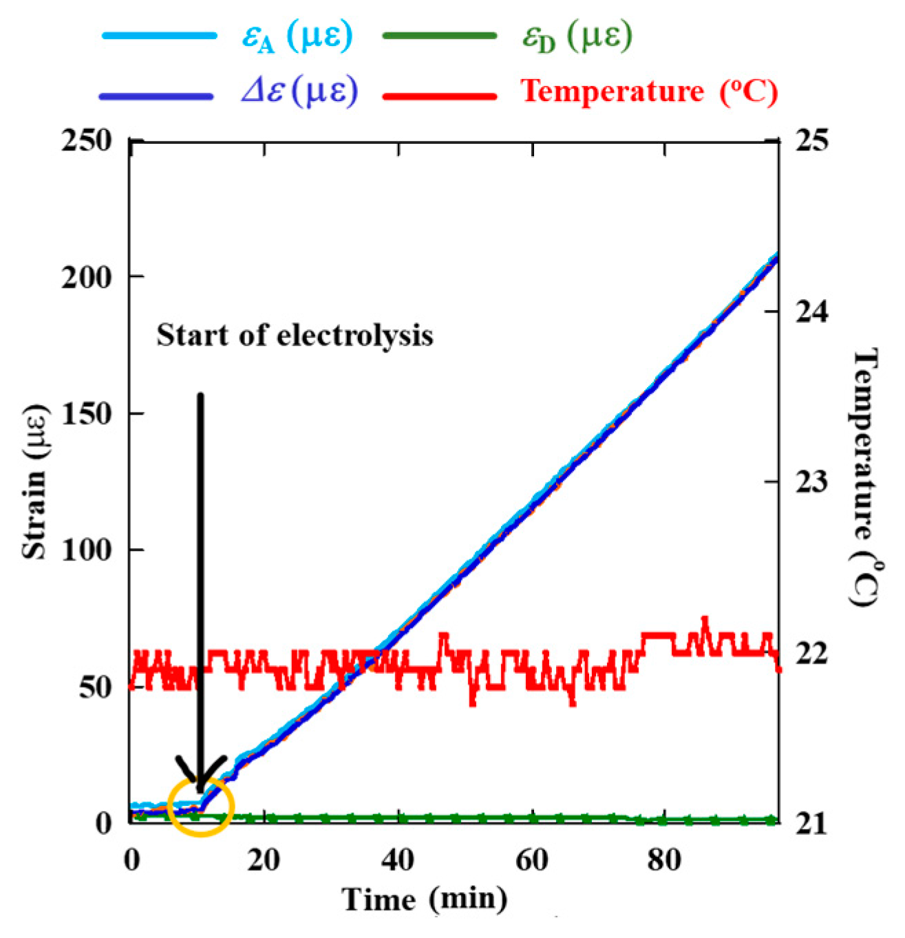
The results obtained by the strain gauge of the amplifier circuit for the ACM sensor during galvanostatic electrolysis are shown in Figure 9. Each voltage reading of the amplifier circuit is converted to strain in advance. The figure shows the time evolution of the strain due to the change in thickness of the test piece. When the ACM sensor was immersed in the reservoir, and the surface of the test piece was placed longitudinally, it was easy for making the corrosion products from the surface during the experiment.
The strain of the active circuit (εA) had a linear signal in terms of elapsed time during electrolysis. The strain value of the dummy circuit (εD) was constant throughout the electrolysis process. Δε is the difference between εA and εD, which were obtained by measurements of the amplifier circuit through the active-dummy method for the ACM sensor. Δε increased linearly with time because given the constant current during the experiment, galvanostatic electrolysis depended on elapsed time. After electrolysis began εA is linearly increased this indicated the compressive strain on the test piece, which became smaller with the decreasing of the thickness of test piece according to Equation (1).
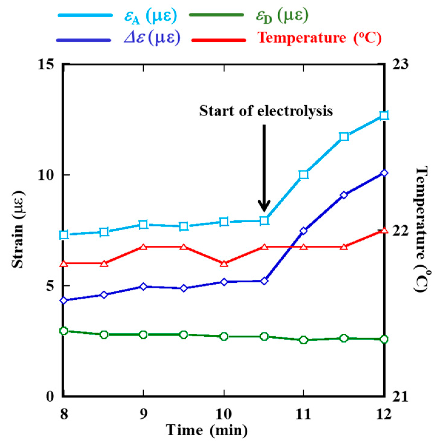
Figure 10 shows a close-up of the results around 10.5 min, when electrolysis began. Before 10.5 min, εA is constant. After 10.5 min, it is smaller owing to the thinning of the test piece. εD is completely unaffected by the signal. It can be concluded that under the active-dummy method, the amplifier circuit for an ACM sensor can measure small values in με, which corresponds to the resolution of the amplifier circuit.
To investigate the accuracy of the amplifier circuit under the active-dummy method, the actual thickness reduction of the test piece was measured. ΔyA is the change in thickness of the test piece, as determined by measuring the actual thickness at five different points on the corroded area of the test piece with a micrometer before and after the experiment. The measurements of the actual thickness were 0.29, 0.28, 0.28, 0.27, and 0.28 mm. The average thickness of the test piece after corrosion was 0.28 mm. Since the initial thickness was 0.48 mm, ΔyA was 0.20 mm.
ΔW is the change in weight of the test piece, as determined from the actual weights measured before and after the experiment and by using the relationship:
where ΔW is the change in weight, S is the corroded area of the test piece, and d is the density of the test piece. In this study, ΔW = 1.42 g, S = 900 mm2, and d = 0.0078 g·mm−3. Furthermore, Δy was obtained via the relationship between Δy and Δε, as described in Section 2.1. The measurement results obtained through the calculations of the actual thickness and actual weight of the test piece are arranged in Table 2. Δy was well aligned with ΔyA and ΔyW, since the errors in the error in these to latter measurements were approximately 12%.
3.3. Strain Due to the Temperature Change of Measurement Environment
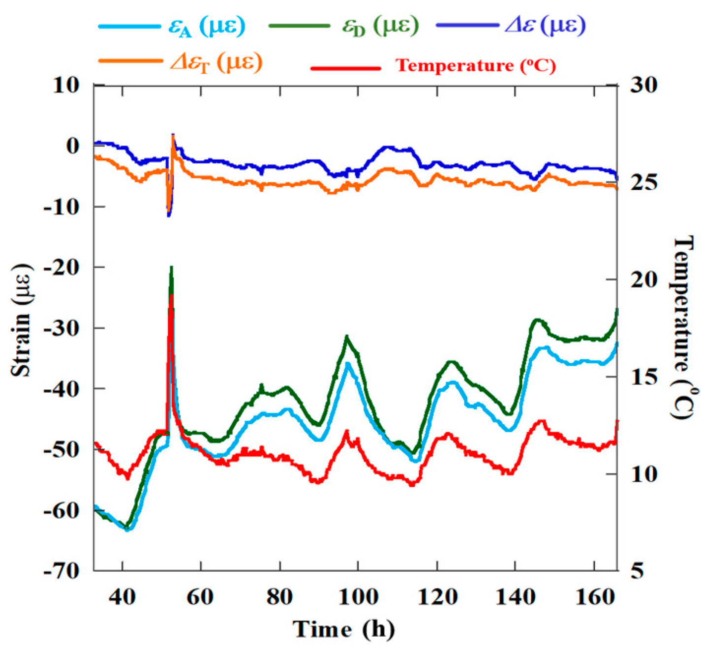
Figure 11 shows the original experiment results starting 166 h before corrosion, as described in Section 2.2.6. It is seen that εA and εD have a similar response to temperature variation. When only the active circuit is used, the variation in εA is high, at about 30 με. The dummy circuit can compensate for the variation by subtracting the same response signal as Δε. The variation in Δε with temperature is small, at less than 10 με. To obtain a more accurate and constant value for Δε, the relationship between temperature and Δε was adjusted.
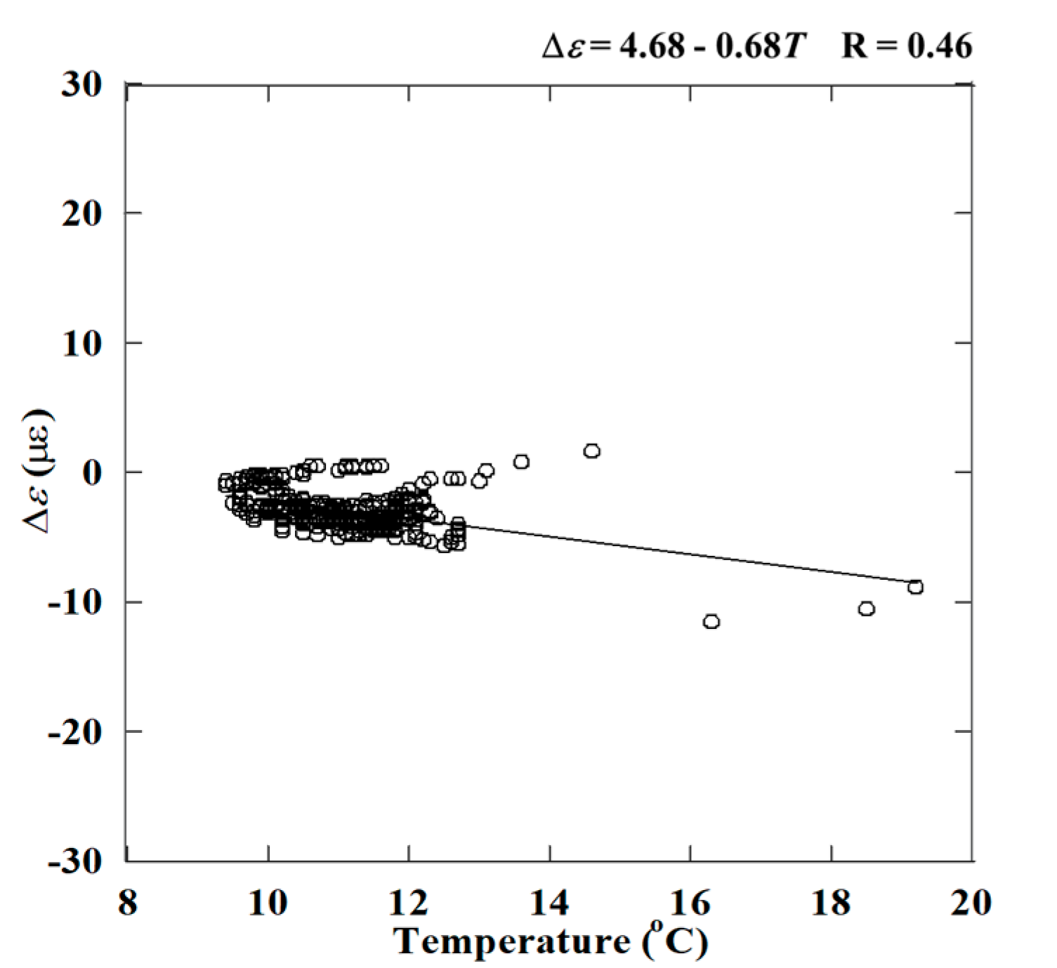
In Figure 12, the effect of temperature on Δε follows the equation of the master curve Δε = 4.68 − 0.68T. This means that temperature shifts Δε by about 0.68 με/°C. By using this equation, Δε was corrected to reduce the effect of the temperature of the measurement environment.
ΔεT is the signal of Δε obtained after the equation for the relationship between temperature and Δε was applied. The value of ΔεT is more constant than Δε.
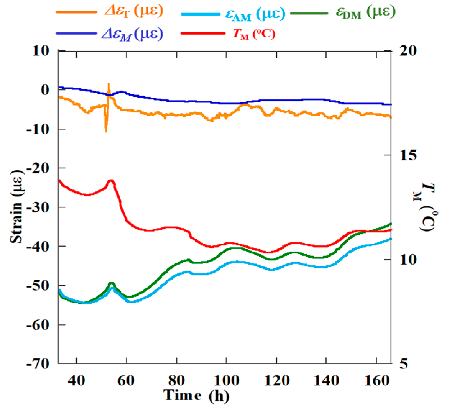
Furthermore, a moving average analysis was conducted. Corrosion is not a rapid process, rather it occurs over long time spans. A moving average analysis, which enables long-time-span analysis of signals, serves to distribute the data. Indeed, as the results in Figure 13 show, the signal obtained is smoother and more constant than the original results.
Figure 13 shows the moving average analysis of the signal pattern of strain using 100 interval data. εAM is the strain of the active circuit after the moving average analysis, and εDM is the strain of the dummy circuit after the moving average analysis. ΔεM is the strain of the amplifier circuit after the moving average analysis, which is obtained from the difference between εDM and εAM. From Figure 13, ΔεM is significantly more constant than ΔεT. This indicates that the moving average is needed in this experiment for accurate measurement without the effect of the temperature variation of the measurement environment.
4. Conclusions
The conclusions of the present study are as follows:
- An amplifier circuit using the active-dummy method for an ACM sensor based on strain measurement was developed. It successfully overcomes the noise from the environment by compensating from the dummy circuit to the active circuit.
- The master curve of strain versus voltage for the newly developed amplifier circuit indicated high sensitivity with a slope of 39 με/V.
- The experiment on the thickness reduction of the test piece by galvanostatic electrolysis revealed strong alignment between the calculated results and the strain measurements made with the amplifier circuit by using the active-dummy method. The error rate was approximately 12%.
- The strain due to temperature variation was obtained via Δε = 4.68 − 0.68T. The effect of temperature on Δε was around 0.68 με/°C.
- ΔεT remained slightly more constant than Δε with temperature variations in the measurement environment.
- ΔεM was significantly more constant than ΔεT, which indicated that the moving average should be used in experiments to obtain more accurate measurements.
- In the field measurement, the corrosion layers of the test piece of the ACM sensor might affect the signals, and its effect would benefit from further study. The relationship of corrosion progression and strain measurement need to be further verified in the future. After developing the ACM sensor system, including an amplifier circuit using the active-dummy method, and unveiling the effect of corrosion layers on the signal, atmospheric corrosion of steel structures can be estimated with an ACM sensor system. The ACM sensor can be installed on different surfaces of the structure.
Acknowledgments
This work was supported by a Grant-in-Aid for Scientific Research (B) JSPS KAKENHI Grant No. 16H03132 and Yokohama National University. In addition, the authors would like to thank the Indonesian Directorate General of Higher Education for their financial support of the author’s study.
Author Contributions
Hiroshi Kihira devised the main conceptual ideas; Naoya Kasai, Hiroshi Kihira and Shinji Okazaki developed the theory and proofs for the outline; Naoya Kasai encouraged Nining Purwasih to investigate and supervised the findings of this work; and Nining Purwasih, Naoya Kasai and Shinji Okazaki designed the model and performed the experiments and analyzed the data. All authors discussed the result and contributed to the final manuscript.
Conflicts of Interest
The authors declare there is no conflict of interest. The supporters did not have a role in the design of the study; in the collection, analyses, and interpretation of data; in the writing of the manuscript, or in the decision to publish the results.
Abbreviations
The following abbreviations are used in this manuscript.
| D | Density of test piece (g·cm−3) |
| dθ | Center angle of curvature of the test piece (°) |
| E | Young’s modulus of the test piece (Pa) |
| RAA | Resistance of active gauge for active circuit (Ω) |
| RAD | Resistance of active gauge for dummy circuit (Ω) |
| RDA | Resistance of dummy gauge for active circuit (Ω) |
| RDD | Resistance of dummy gauge for dummy circuit (Ω) |
| RVR | Resistance of variable resistor (Ω) |
| S | Corroded area of test piece (cm2) |
| SG | Strain gauge for measuring the strain by commercial strain (-) |
| T | Temperature (°C) |
| TM | Temperature with moving average analysis (°C) |
| VA | Output voltage of active circuit (V) |
| VBA | Output voltage of bridge circuit of active circuit (mV) |
| VBD | Output voltage of bridge circuit of dummy circuit (mV) |
| VCC | Positive input voltage for op-amp (V) |
| VD | Output voltage of dummy circuit (V) |
| VEE | Negative input voltage for op-amp (V) |
| VIN | Input voltage for bridge circuit (V) |
| Vp-p | Peak-to-peak voltage (V) |
| Y | Test piece thickness (m) |
| ΔV | Difference between the output voltages of the active and dummy circuits (V) |
| ΔW | Actual weight obtained by analysis (g) |
| Δy | Change in thickness of test piece (m) |
| ΔyA | Actual thickness obtained by analysis (μm) |
| ΔyW | Actual thickness obtained by electrochemical analysis (μm) |
| Δε | Differential strain (με) |
| ΔεM | Differen ce in strain between the active and dummy circuits, determined by moving average analysis (με) |
| ΔεT | Difference in strain, taking account of the temperature effect (με) |
| ε | Strain in test piece (-) |
| εA | Strain of the active circuit (με) |
| εAM | Strain of the active circuit obtained by moving average analysis (με) |
| εAT | Strain of active circuit, taking account of the temperature effect (με) |
| εD | Strain of dummy circuit (με) |
| εDM | Strain of dummy circuit obtained by moving average analysis (με) |
| εDT | Strain of dummy circuit, taking account of temperature effect (με) |
| εm | Strain with input only from signal (-) |
| εm,t,o | Strain with input from signal and environmental factors (-) |
| εt,o | Strain with input only from environmental factors (-) |
| ρ | Radius of curvature of test piece (m) |
| σy | Yield stress of test piece (Pa) |
References
- Alamin, M.; Tian, G.Y.; Andrews, A.; Jackson, P. Corrosion detection using low-frequency RFID technology. Insight-Non-Destr. Test. Cond. Monit. 2012, 54, 72–75. [Google Scholar] [CrossRef]
- Zhang, H.; Yang, R.; He, Y.; Tian, G.Y.; Xu, L.; Wu, R. Identification and characterization of steel corrosion using passive high frequency RFID sensors. Measurement 2016, 92, 421–427. [Google Scholar] [CrossRef]
- Zhang, J.; Tian, G.Y.; Marindra, A.M.J.; Sunny, A.I.; Zhao, A.B. A review of passive RFID tag antenna-based sensors and systems for structural health monitoring applications. Sensors 2017, 17, 265. [Google Scholar] [CrossRef] [PubMed]
- Gattan, S.K.T.; Taylor, S.E.; Sun, T.; Basheer, P.A.M.; Grattan, K.T.V. Monitoring of corrosion in structural reinforcing bars: Performance comparison using in situ fiber-optic and electric wire strain gauge systems. IEEE Sens. J. 2009, 9, 1494–1502. [Google Scholar] [CrossRef]
- Hu, W.; Cai, H.; Yang, M.; Tong, X.; Zhou, C.; Chen, W. Fe-C-coated fibre Bragg grating sensor for steel corrosion monitoring. Corros. Sci. 2011, 53, 1933–1938. [Google Scholar] [CrossRef]
- Zang, N.; Chen, W.; Zheng, X.; Hu, W.; Gao, M. Optical sensor for steel corrosion monitoring based on etched Fiber Bragg Grating sputtered with iron film. IEEE Sens. J. 2015, 15, 3511–3556. [Google Scholar]
- Al Handawi, K.; Vahdati, N.; Rostron, P.; Lawand, L.; Shiryayev, O. Strain based FBG sensor for real-time corrosion rate monitoring in pre-stressed structures. Sens. Actuator B 2016, 236, 276–285. [Google Scholar] [CrossRef]
- Almubaied, O.; Chai, H.K.; Islam, M.R.; Lim, K.; Tan, C.G. Monitoring corrosion process of reinforced concrete structure using FBG strain sensor. IEEE Trans. Instrum. Meas. 2017, 66, 2148–2155. [Google Scholar] [CrossRef]
- Mansfeld, F.; Kenkel, J.V. Electrochemical monitoring of atmospheric corrosion phenomena. Corros. Sci. 1976, 16, 111–112. [Google Scholar] [CrossRef]
- Mansfeld, F.; Tsai, S. Laboratory studies of atmospheric corrosion—I. Weight loss and electrochemical measurements. Corros. Sci. 1980, 20, 853–872. [Google Scholar] [CrossRef]
- Ridha, M.; Fonna, S.; Huzni, S.; Supardi, J.; Ariffin, A.K. Atmospheric corrosion of structural steels exposed in the 2004 tsunami-affected areas of Aceh. IJAME 2013, 7, 1014–1022. [Google Scholar] [CrossRef]
- Monsada, A.M.; Margarito, M.T.; Milo, L.C.; Casa, E.P.; Zabala, J.V.; Maglines, A.S.; Basilia, B.A.; Harada, S.; Shinohara, T. Atmospheric corrosion exposure study of The Philippine Historical all steel Basilica. Zairyo Kankyo 2016, C-107, 267–270. [Google Scholar]
- Dara, T.; Shinohara, T.; Umezawa, O. The Behavior of corrosion of low carbon steel affected by corrosion product and Na2SO4 concentration under artificial rainfall test. Zairyo Kankyo 2016, C-114, 298–302. [Google Scholar]
- Lien, L.T.H.; Hong, H.L.; San, P.T.; Hieu, N.T.; Nga, N.T.T. Atmospheric corrosion of carbon steel and weathering steel—Relation of corrosion and environmental factors. Zairyo Kankyo 2016, C-110, 280–284. [Google Scholar]
- Odara, T.; Tahara, A.; Dara, T. Atmospheric corrosion behaviors of steels in Japan. Zairyo Kankyo 2016, C-111, 285–288. [Google Scholar]
- Viyanit, E.; Pongsaksawad, W.; Sorachot, S.; Matsuyama, H.; Fukuda, N. Investigation of atmospheric corrosion behavior of austenitic and ferritic stain less steel welds under tropical climate of Thailand. Zairyo Kankyo 2016, C-109, 275–279. [Google Scholar]
- Mansfeld, F.; Jeanjaquet, S.L.; Kendig, M.W.; Roe, D.K. A new atmospheric corrosion rate monitor development and evaluation. Atmos. Environ. 1986, 20, 1179–1192. [Google Scholar] [CrossRef]
- Nishikata, A.; Yamashita, Y.; Katayama, H.; Tsuru, T.; Usami, A.; Tanabe, K.; Mabuchi, H. An electrochemical impedance study on atmospheric corrosion of steels in a cyclic wet–dry condition. Corros. Sci. 1995, 37, 2059–2069. [Google Scholar] [CrossRef]
- Nishikata, A.; Suzuki, F.; Tsuru, T. Corrosion monitoring of nickel-containing steels in marine atmospheric environment. Corros. Sci. 2005, 47, 2578–2588. [Google Scholar] [CrossRef]
- Cruz, R.P.V.; Nishikata, A.; Tsuru, T. AC impedance monitoring of pitting corrosion of stainless steel under a wet–dry cyclic condition in chloride-containing environment. Corros. Sci. 1996, 38, 1397–1406. [Google Scholar] [CrossRef]
- El-Mahdy, G.A.; Nishikata, A.; Tsuru, T. Electrochemical corrosion monitoring of galvanized steel under cyclic wet–dry conditions. Corros. Sci. 2000, 42, 183–194. [Google Scholar] [CrossRef]
- Yadav, A.P.; Nishikata, A.; Tsuru, T. Electrochemical impedance study on galvanized steel corrosion under cyclic wet–dry conditions-influence of time of wetness. Corros. Sci. 2004, 46, 169–181. [Google Scholar] [CrossRef]
- Yadav, A.P.; Suzuki, F.; Nishikata, A.; Tsuru, T. Investigation of atmospheric corrosion of Zn using ac impedance and differential pressure meter. Electrochim. Acta 2004, 49, 2725–2729. [Google Scholar] [CrossRef]
- El-Mahdy, G.A.; Nishikata, A.; Tsuru, T. AC impedance study on corrosion of 55% Al–Zn alloy-coated steel under thin electrolyte layers. Corros. Sci. 2000, 42, 1509–1521. [Google Scholar] [CrossRef]
- Dong, J.H.; Chen, W.; Ke, W. Corrosion evolution of steel simulated of SO2 polluted coastal atmospheres, Zairyo Kankyo 2016, C-112, 289–292. Zairyo Kankyo 2016, C-112, 289–292. [Google Scholar]
- Thee, C.; Dong, J.; Ke, W. Corrosion monitoring of weathering steel in a simulated coastal-industrial environment. Int. J. Environ. Chem. Ecol. Geol. Geophys. Eng. 2015, 9, 587–593. [Google Scholar]
- Parson, N.; Khamsuk, P.; Sorachot, S.; Khonraeng, W.; Wongpinkaew, K.; Kaewkumsai, S.; Pongsaksawad, W.; Viyanit, E.; Chianpairot, A. Atmospheric corrosion of structural steels in Thailand Tropical Climate. Zairyo Kankyo 2016, C-108, 271–274. [Google Scholar]
- Li, C.; Ma, Y.; Li, Y.; Wang, F. EIS monitoring study of atmospheric corrosion under variable relative. Corros. Sci. 2010, 52, 3677–3686. [Google Scholar] [CrossRef]
- Shitanda, I.; Okumura, A.; Itagaki, M.; Watanabe, K.; Asano, Y. Screen-printed atmospheric corrosion monitoring sensor based on electrochemical impedance spectroscopy. Sens. Actuators B 2009, 139, 292–297. [Google Scholar] [CrossRef]
- Cai, J.P.; Lyon, S.B. A mechanistic study of initial atmospheric corrosion kinetics using electrical resistance sensor. Corros. Sci. 2005, 47, 2956–2973. [Google Scholar] [CrossRef]
- Li, S.; Kim, Y.G.; Jung, S.; Song, H.S.; Lee, S.M. Application of steel thin film electrical resistance sensor for in situ corrosion monitoring. Sens. Actuators B 2007, 120, 368–377. [Google Scholar] [CrossRef]
- He, Y.; Tian, G.; Zhang, H.; Alamain, M.; Simm, A.; Jackson, P. Steel corrosion characterization using pulsed eddy current systems. IEEE Sens. J. 2012, 12, 2113–2120. [Google Scholar] [CrossRef]
- Yasri, M.; Gallee, F.; Lescop, B.; Diler, E.; Thierry, D.; Rioual, S. Passive wireless sensor for atmospheric corrosion monitoring. In Proceedings of the 8th European Conference on Antennas and Propagation (EuCAP), The Hague, The Netherlands, 6–11 April 2014; pp. 2945–2949. [Google Scholar]
- Lin, A.N.; Saito, R.; Takaya, S.; Miyagawa, T. Determination of Young’s Modulus of Rush-Layer by Bending Experiment; Technical Paper; JCI: Tokyo, Japan, 2013; Volume 35, pp. 1117–1122. [Google Scholar]
- Kasai, N.; Hiroki, M.; Yamada, T.; Kihira, H.; Matsuoka, K.; Kuriyama, Y.; Okazaki, S. Atmospheric corrosion sensor based on strain measurement. Meas. Sci. Technol. 2017, 28, 15106. [Google Scholar] [CrossRef]
- Kasai, N.; Utatsu, K.; Park, S.; Kitsukawa, S.; Sekine, K. Correlation between corrosion rate and AE signal in an acidic environment for mild steel. Corros. Sci. 2009, 51, 1679–1684. [Google Scholar] [CrossRef]
Figure 1.
Schematic of test piece subjected to moments M and M’. (a) Initial conditions; (b) after the test piece thickness decreases upon corrosion.
Figure 1.
Schematic of test piece subjected to moments M and M’. (a) Initial conditions; (b) after the test piece thickness decreases upon corrosion.

Figure 2.
Design concept of the active-dummy method.
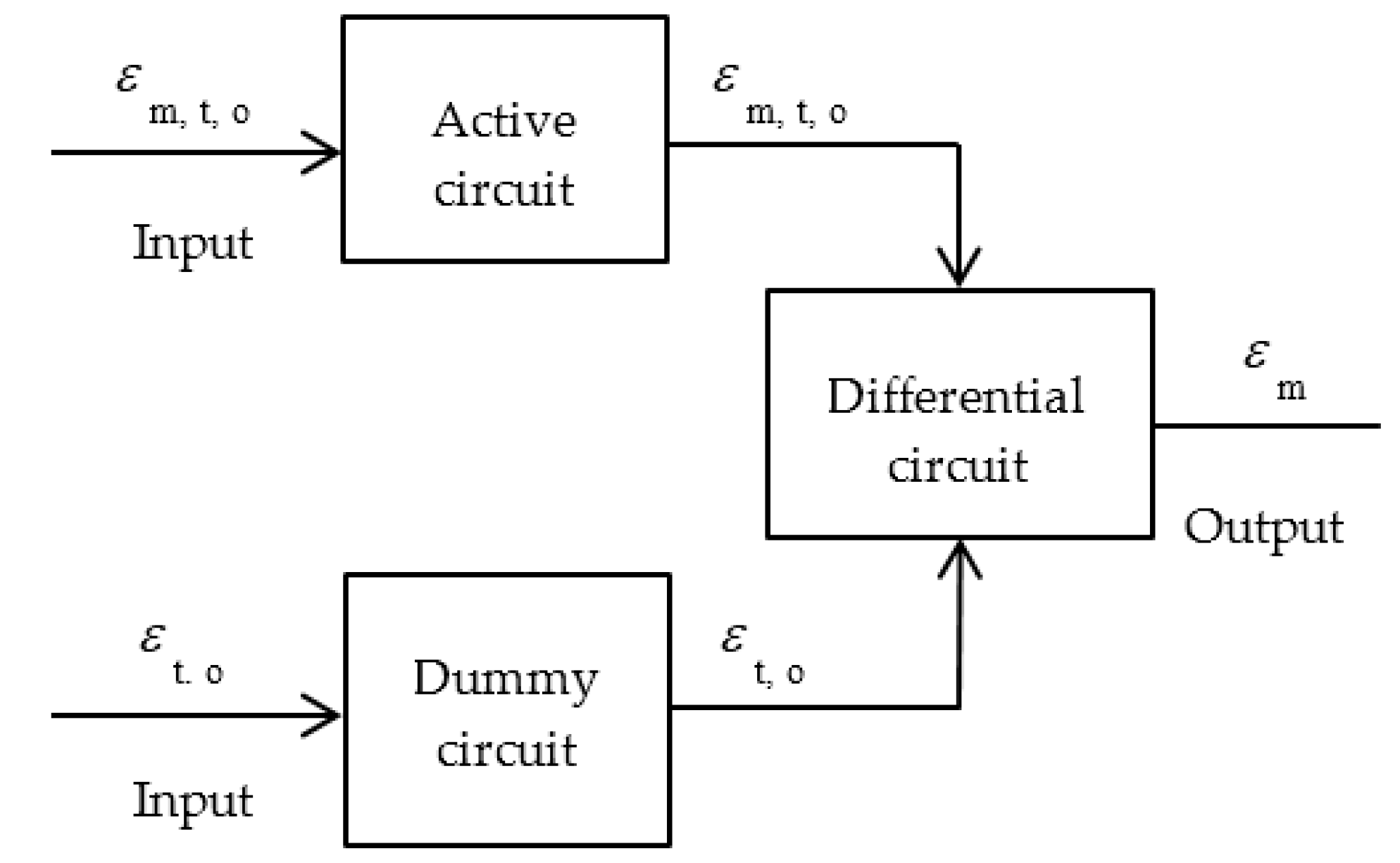
Figure 3.
Test piece and apparatus for ACM (atmospheric corrosion monitoring) sensor. The apparatus comprises of a base, test piece, and cover. A corroded area, 30 mm in length and 30 mm in width, was formed at the center of the test piece; the remaining area was uncorroded.
Figure 3.
Test piece and apparatus for ACM (atmospheric corrosion monitoring) sensor. The apparatus comprises of a base, test piece, and cover. A corroded area, 30 mm in length and 30 mm in width, was formed at the center of the test piece; the remaining area was uncorroded.

Figure 4.
Configuration of strain gauges on test piece for ACM sensor. (a) TPA with 900 mm2 corroded area at the center and the remaining area uncorroded; (b) TPD, with the entire test piece uncorroded.
Figure 4.
Configuration of strain gauges on test piece for ACM sensor. (a) TPA with 900 mm2 corroded area at the center and the remaining area uncorroded; (b) TPD, with the entire test piece uncorroded.
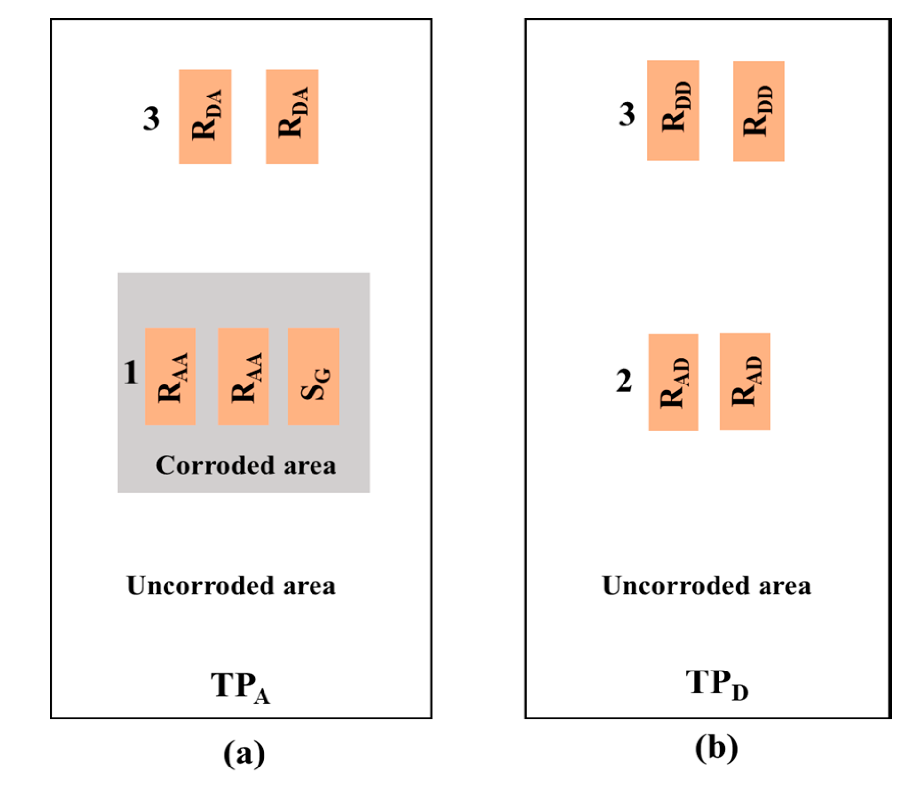
Figure 5.
Design of the amplifier circuit by the active-dummy method.

Figure 6.
Photograph of the amplifier circuit by the active-dummy method.

Figure 7.
Experimental setup for measuring the thinning of a test piece by galvanostatic electrolysis.
Figure 7.
Experimental setup for measuring the thinning of a test piece by galvanostatic electrolysis.
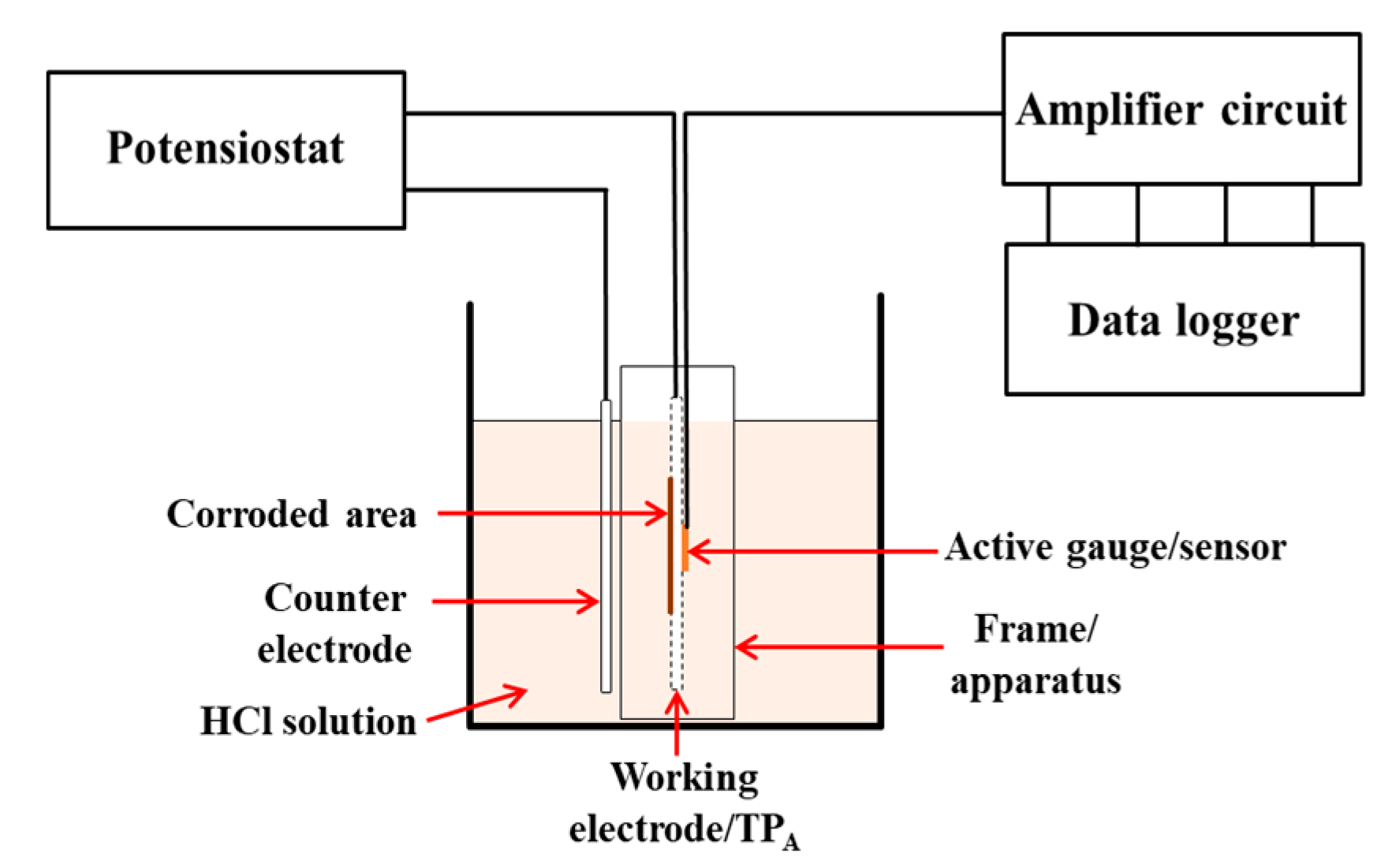
Figure 8.
Master curve of strain vs. voltage.
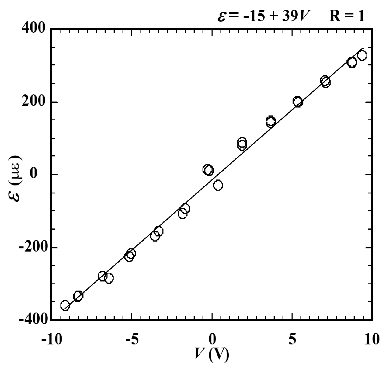
Figure 9.
Strain signal pattern as a function of elapsed time during electrolysis process.

Figure 10.
Close-up of Figure 9 around the start of the electrolysis process.
Figure 10.
Close-up of Figure 9 around the start of the electrolysis process.

Figure 11.
Signal pattern before corrosion is applied.

Figure 12.
Relationship between the voltage and temperature.

Figure 13.
Signal pattern of the voltage before corrosion is applied with the moving average.


Table 1.
Position and purpose of strain gauges in Figure 4.
Table 1.
Position and purpose of strain gauges in Figure 4.
| Positions of Strain Gauges | Active Circuit | Dummy Circuit |
|---|---|---|
| Active Strain Gauge | RAA: Corroded area with bending. Detects signals due to corrosion-induced thinning of test piece. | RAD: Uncorroded without bending. Detects signals without thinning of test piece. |
| Dummy Strain Gauge | RDA: Uncorroded area without bending. Compensates for effects of environmental conditions on RAA. | RDD: Uncorroded area without bending. Compensates for effects of environmental conditions on RAD. |
| Strain Gauge | SG: At the center of corroded area without bending. Measures the strain in the corroded area with commercial strain measurement device. | |
Table 2.
Determination of thickness reduction from measured strain, thickness, and weight.
| Parameters of Thickness Reduction | Δy | ΔyA | ΔyW |
|---|---|---|---|
| Thickness (μm) | 177 | 200 | 202 |
| Error (%) | - | 11 | 12 |
© 2017 by the authors. Licensee MDPI, Basel, Switzerland. This article is an open access article distributed under the terms and conditions of the Creative Commons Attribution (CC BY) license (http://creativecommons.org/licenses/by/4.0/).
Share and Cite
MDPI and ACS Style
Purwasih, N.; Kasai, N.; Okazaki, S.; Kihira, H. Development of Amplifier Circuit by Active-Dummy Method for Atmospheric Corrosion Monitoring in Steel Based on Strain Measurement. Metals 2018, 8, 5. https://doi.org/10.3390/met8010005
AMA Style
Purwasih N, Kasai N, Okazaki S, Kihira H. Development of Amplifier Circuit by Active-Dummy Method for Atmospheric Corrosion Monitoring in Steel Based on Strain Measurement. Metals. 2018; 8(1):5. https://doi.org/10.3390/met8010005
Chicago/Turabian StylePurwasih, Nining, Naoya Kasai, Shinji Okazaki, and Hiroshi Kihira. 2018. "Development of Amplifier Circuit by Active-Dummy Method for Atmospheric Corrosion Monitoring in Steel Based on Strain Measurement" Metals 8, no. 1: 5. https://doi.org/10.3390/met8010005
Note that from the first issue of 2016, this journal uses article numbers instead of page numbers. See further details here.