Development of a Façade Assessment and Design Tool for Solar Energy (FASSADES)


Abstract
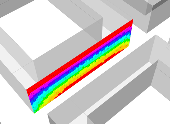
:
1. Introduction
2. Method
2.1. Steps 1 and 2

2.2. Step 3
2.2.1. Step 3a

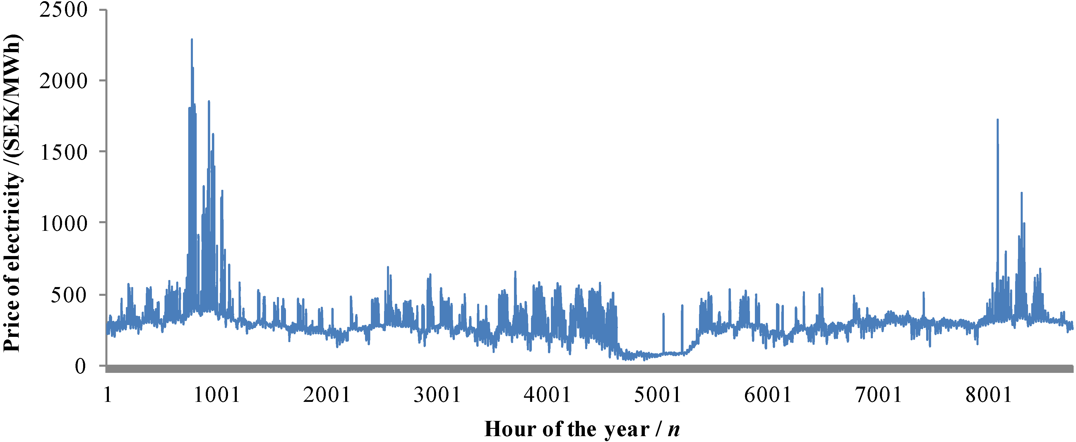
| Weather data | Copenhagen EPW | |
|---|---|---|
| Reflectances | Ground | 20% |
| Buildings | 35% | |
| Energy + simulations: | Time steps per hour: | 6 |
| Time period | Annual | |
| Reflections | Full exterior with reflections | |
| Output | Zone Beam Solar from Exterior Windows Energy and Zone Diffuse Solar from Exterior Windows Energy | |
| Radiance simulations: | Nodes offset | 10 mm |
| Ambient bounces | 10 | |
| Ambient divisions | 1000 | |
| Ambient super-samples | 20 | |
| Ambient resolution | 300 | |
| Ambient accuracy | 0.1 | |

2.2.2. Step 3b

2.2.3. Step 3c

- Direct irradiation (W/m2);
- Diffuse irradiation (W/m2);
- Incidence angle (°);
- Ambient temperature (°C);
- Features of a solar panel. The following parameters were obtained by comparing several ST product specifications [28]:
- F’(τα)n: 0.851 (–);
- Kd: 0.9 (–);
- F’U1: 4.036 (W/m2K);
- F’U2: 0.0108 (W/m2K2);
- B0: 0.09 (–).
2.2.4. Step 4

| Provider | Fortum a | Mälar Energi b | Vattenfall c | Göteborgs Energi d | Öresunds-kraft e | EON f | Average |
|---|---|---|---|---|---|---|---|
| Jan | 714 | 440 | 748 | 503 | 866 | 559 | 638 |
| Feb | 714 | 440 | 748 | 503 | 866 | 559 | 638 |
| Mar | 714 | 388 | 748 | 503 | 866 | 559 | 630 |
| Apr | 469 | 388 | 748 | 346 | 485 | 161 | 433 |
| May | 285 | 292 | 309 | 99 | 485 | 161 | 272 |
| Jun | 285 | 292,00 | 309 | 99 | 123 | 161 | 211 |
| Jul | 285 | 292,00 | 309 | 99 | 123 | 161 | 211 |
| Aug | 285 | 292,00 | 309 | 99 | 123 | 161 | 211 |
| Sep | 285 | 292,00 | 309 | 99 | 123 | 161 | 211 |
| Oct | 469 | 292,00 | 748 | 346 | 123 | 370 | 391 |
| Nov | 469 | 388,00 | 748 | 346 | 485 | 370 | 468 |
| Dec | 714 | 440,00 | 748 | 503 | 866 | 559 | 638 |
2.3. Step 5
ΨST = σ·Q
3. Results

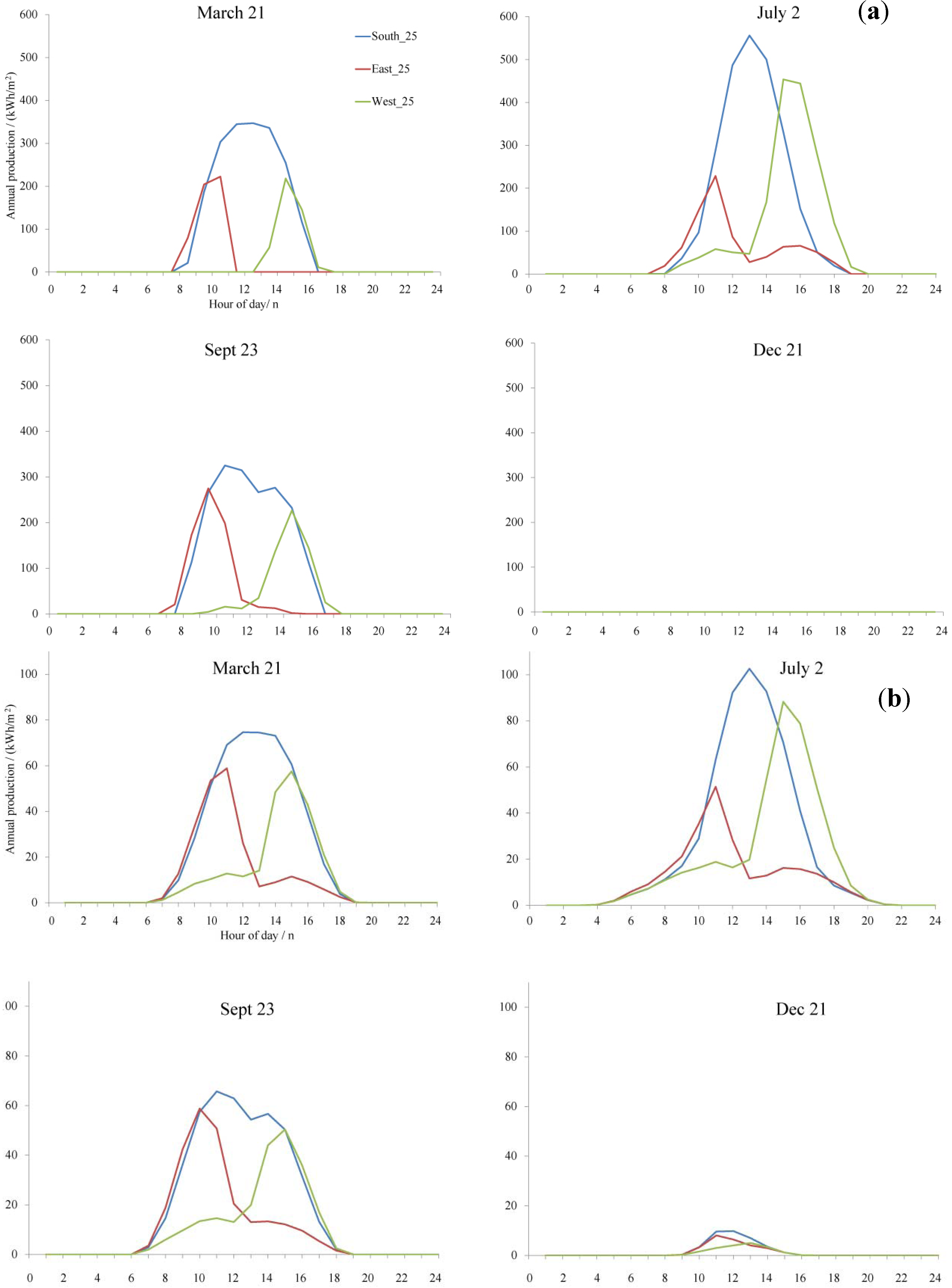
3.1. Annual and Hourly Production of the Whole Façade
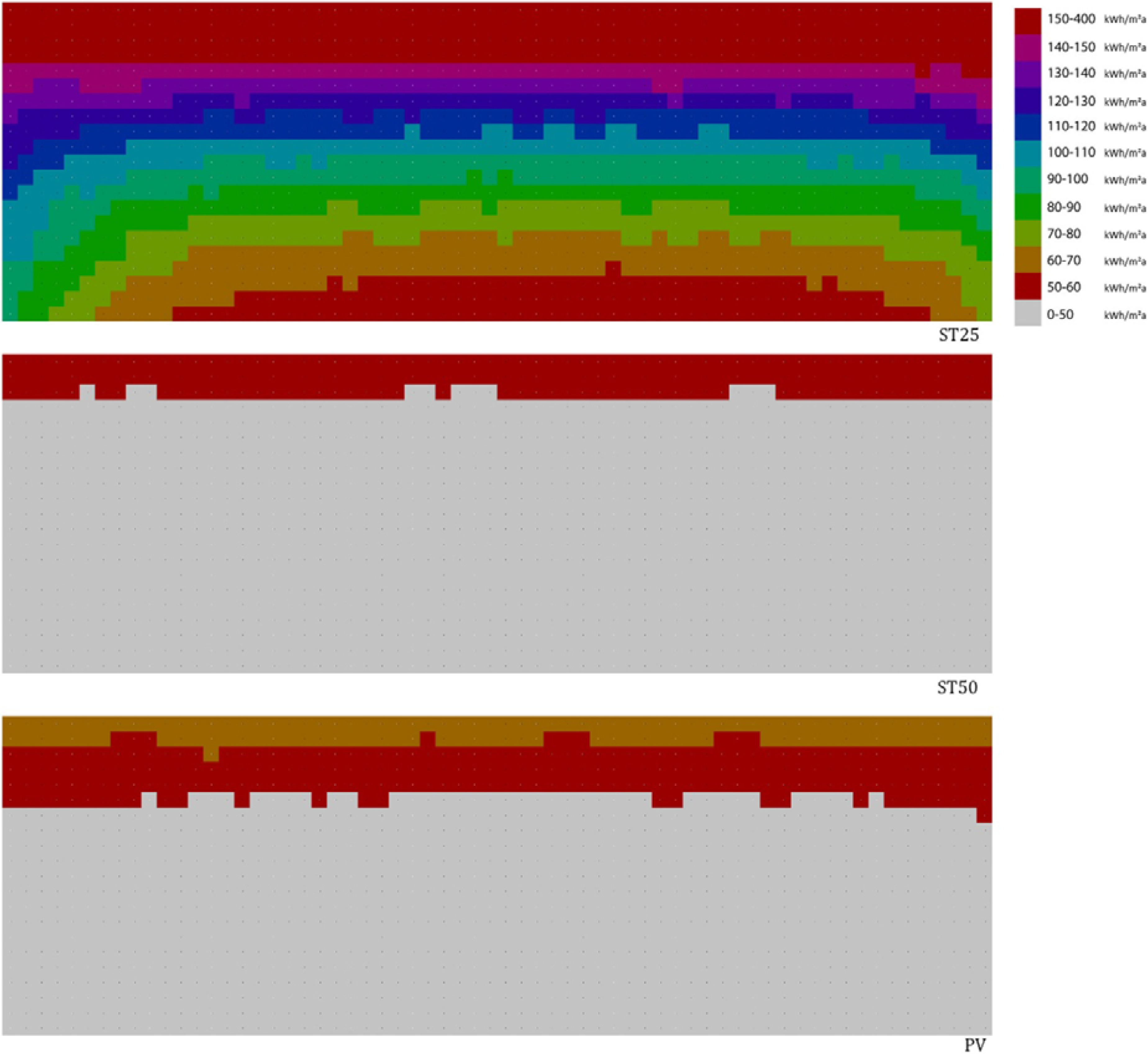
- The production of 90 °C heat is very limited and is even 0 kWh on the North façade, due to the relative low irradiation in Sweden;
- The difference between the solar thermal production at 25 °C and ST with the other system temperatures and PV is significant. For example, at z = 19.5 m, the ST production at 25 °C is 314 kWh/m2a, the production of ST at 50 °C is 45% of this value, at 75 °C, it is 21% of this value, at ST 90 °C, 13%, and for PV, the production corresponds to only 29% of the ST 25 °C production. Note also that the ST production (25 °C) on East and West facades is higher than the PV production on the South façade;
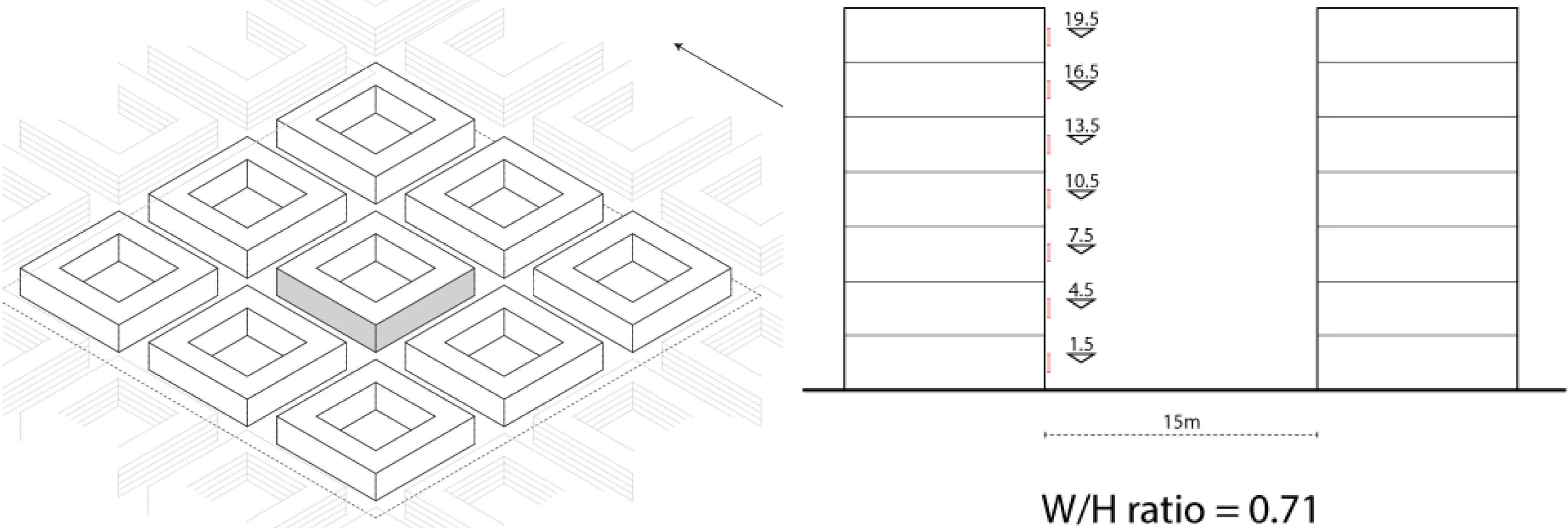
- Shading due to surrounding buildings has a significant impact on the solar energy production. The production of almost all technologies decreases by 50%–70% for lower positions (e.g., 1.5 m) compared to the higher ones (e.g., 19.5 m). This shading effect was also observed in an earlier study [3].


- In the morning, production from the East façade is slightly higher than from the South façade (until 09.00), although differences are very small. In the afternoon, the production from the West façade is higher than the production from the two other facades, especially on 2 July, when the production is notably higher. During the majority of the day, the production from the South façade is higher than from the East and West façades;
- On 21 December, there is no production of solar heat (25 °C) and hardly any production of PV.
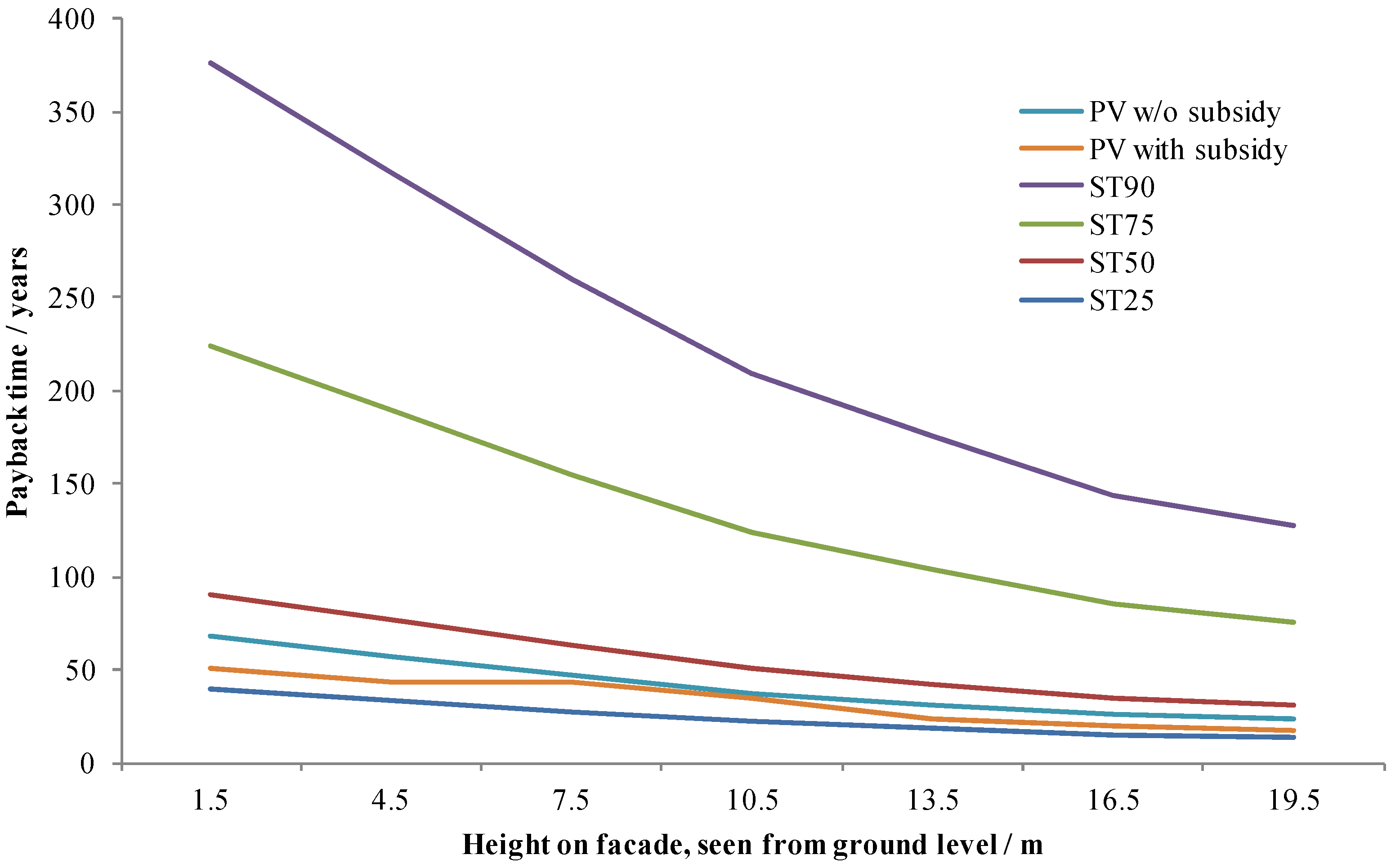
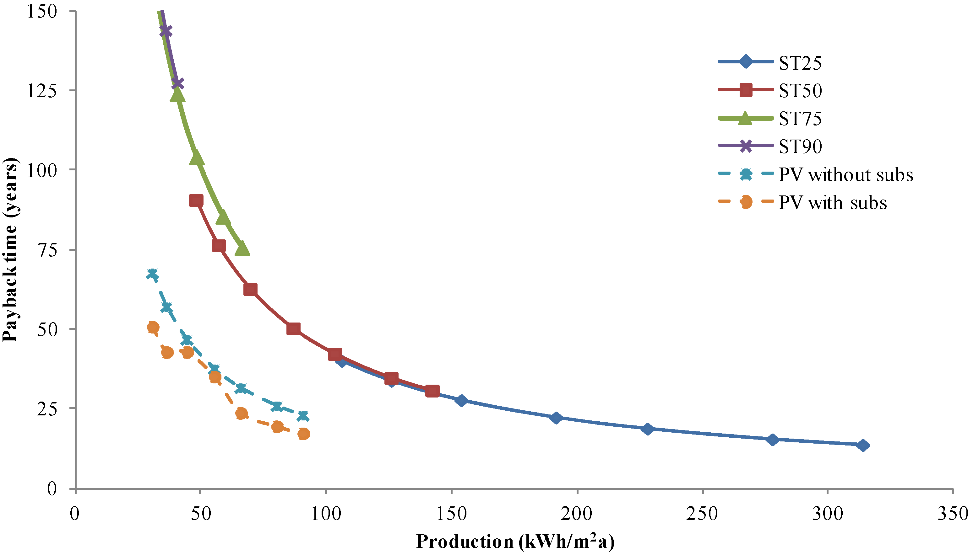
3.2. Assessment of the Whole Façade

- Installing a ST system providing a system temperature 50 °C, 75 °C, and 90 °C is not financially interesting, since it is unlikely to produce sufficiently on facades;
- Installing a ST system delivering 25 °C heat is economically interesting, especially at higher levels on the façade;
- Installing PV on the façade can be economically interesting, especially with subsidy and on the higher levels of the façade. The differences between subsidised and non-subsidised PV cells are relatively small in the graph, probably because the subsidy is proportional to the investment (Figure 9).

| Years | 25 | 20 | 15 | 10 | 5 |
|---|---|---|---|---|---|
| ST25 | 170 | 213 | 284 | 425 | 851 |
| ST50 | 175 | 218 | 291 | 437 | 873 |
| ST75 | 201 | 252 | 335 | 503 | 1006 |
| ST90 | 208 | 260 | 347 | 520 | 1040 |
| PV w/o | 83 | 104 | 139 | 208 | 416 |
| PV with | 76 | 95 | 126 | 189 | 378 |
| Orientation of façade/system temperature | ST 25 °C | ST 50 °C | ST 75 °C | ST 90 °C | PV (SE4) |
|---|---|---|---|---|---|
| South (averaged) | 0.35 | 0.34 | 0.30 | 0.29 | 0.80 |
| East (averaged) | 0.32 | 0.32 | 0.27 | 0.26 | 0.80 |
| West (averaged) | 0.31 | 0.31 | 0.27 | 0.27 | 0.79 |
| North (averaged) | 0.28 | N/A | N/A | N/A | 0.80 |
4. Conclusions
Acknowledgments
Author Contributions
Conflicts of Interest
References
- Directive 2010/31/EU of the European Parliament and of the Council; European Commission: Brussels, Belgium, 2010.
- Sartori, I.; Napolitano, A.; Marszal, A.; Pless, S.; Torcelli, I.; Voss, K. Criteria for Definintion of Net Zero Energy Buildings. In Proceedings of the International Conference on Solar Heating, Cooling and Buildings (EuroSun 2010), Graz, Austria, 28 September–1 October 2010.
- Kanters, J.; Horvat, M. Solar energy as a design parameter in urban planning. Energy Procedia 2012, 30, 1143–1152. [Google Scholar] [CrossRef]
- Kanters, J.; Wall, M.; Dubois, M.-C. Typical values for active solar energy in urban planning. Energy Procedia 2013, in press. [Google Scholar]
- Wall, M.; Snow, M.; Dahlberg, J.; Lundgren, M.; Lindkvist, C.; Wyckmans, A.; Siems, T.; Simon, K. Task 51: Solar Energy in Urban Planning. Available online: http://task51.iea-shc.org/ (accessed on 1 September 2013).
- Kanters, J.; Wall, M.; Kjellsson, E. The solar map as a knowledge base for solar energy use. Energy Procedia 2013, in press. [Google Scholar]
- Jakubiec, J.A.; Reinhart, C.F. A method for predicting city-wide electricity gains from photovoltaic panels based on LiDAR and GIS data combined with hourly daysim simulations. Sol. Energy 2013, 93, 127–143. [Google Scholar] [CrossRef]
- Redweik, P.; Catita, C.; Brito, M. Solar energy potential on roofs and facades in an urban landscape. Sol. Energy 2013, 97, 332–341. [Google Scholar] [CrossRef]
- Dubois, M.-C.; Horvat, M. State-of-The-Art of Digital Tools Used by Architects for Solar Design; International Energy Agency Solar Heating and Cooling Programme; International Energy Agency: Paris, France, 2010. [Google Scholar]
- Horvat, M.; Dubois, M.-C.; Wall, M. DB3. Guidelines for Computer Tools Developers to Sustain Solar Architecture. Techical Report from International Energy Agency Solar Heating and Cooling Programme. 2012. Available online: http://task41.iea-shc.org/data/sites/1/publications/T41B4-final-27Jun2012.pdf/ (accessed on 1 September 2012).
- Kanters, J.; Horvat, M.; Dubois, M.-C. Tools and methods used by architects for solar design. Energy Build. 2014, 68, 721–731. [Google Scholar] [CrossRef]
- Crawley, D.B.; Hand, J.W.; Kummert, M.; Griffith, B.T. Contrasting the capabilities of building energy performance simulation programs. Build. Environ. 2008, 43, 661–673. [Google Scholar] [CrossRef] [Green Version]
- Ibara, D.; Reinhart, C. Solar Availability: A Comparison Study of Six Irradiation Distribution Methods. In Proceedings of the 12th Conference of International Building Performance Simulation Association, Sydney, Australia, 14–16 November 2011.
- Jakubiec, A.; Reinhart, C. DIVA 2.0: Integrating Daylight and Thermal Simulations Using Rhinoceros 3D, Daysim and EnergyPlus. In Proceedings of the 12th Conference of International Building Performance Simulation Association, Sydney, Australia, 14–16 November 2011.
- Fartaria, T.O.; Pereira, M.C. Simulation and computation of shadow losses of direct normal, diffuse solar radiation and albedo in a photovoltaic field with multiple 2-axis trackers using ray tracing methods. Sol. Energy 2013, 91, 93–101. [Google Scholar] [CrossRef]
- Sharma, V.; Chandel, S.S. Performance analysis of a 190 kWp grid interactive solar photovoltaic power plant in India. Energy 2013, 55, 476–485. [Google Scholar] [CrossRef]
- Wills, A.; Cruickshank, C.A.; Beausoleil-Morrison, I. Application of the ESP-r/TRNSYS co-simulator to study solar heating with a single-house scale seasonal storage. Energy Procedia 2012, 30, 715–722. [Google Scholar] [CrossRef]
- Terziotti, L.T.; Sweet, M.L.; McLeskey, J.T., Jr. Modeling seasonal solar thermal energy storage in a large urban residential building using TRNSYS 16. Energy Build. 2012, 45, 28–31. [Google Scholar] [CrossRef]
- Bernardo, L.R.; Davidsson, H.; Karlsson, B. Retrofitting domestic hot water heaters for solar water heating systems in single-family houses in a cold climate: A theoretical analysis. Energies 2012, 5, 4110–4131. [Google Scholar] [CrossRef]
- Rhinoceros 5.0, McNeel: Seattle, WA, USA, September 2013.
- Grasshopper, McNeel: Seattle, WA, USA, September 2013.
- EnergyPlus 8.1, U.S. Department of Energy: Washington, DC, USA, 2013.
- Robinson, D.; Stone, A. Irradiation Modelling Made Simple: The Cumulative Sky Approach and Its Applications. In Proceedings of the 21th Conference on Passive and Low Energy Architecture (Plea2004), Eindhoven, The Netherlands, 19–22 September 2004.
- Hachem, C.; Athienitis, A.; Fazio, P. Parametric investigation of geometric form effects on solar potential of housing units. Sol. Energy 2011, 85, 1864–1877. [Google Scholar] [CrossRef]
- Crawley, D.B.; Lawrie, L.K.; Winkelmann, F.C.; Buhl, W.F.; Huang, Y.J.; Pedersen, C.O.; Strand, R.K.; Liesen, R.J.; Fisher, D.E.; Witte, M.J.; et al. EnergyPlus: Creating a new-generation building energy simulation program. Energy Build. 2001, 33, 319–331. [Google Scholar] [CrossRef]
- Rempel, A.R.; Rempel, A.W.; Cashman, K.V.; Gates, K.N.; Page, C.J.; Shaw, B. Interpretation of passive solar field data with EnergyPlus models: Un-conventional wisdom from four sunspaces in Eugene, Oregon. Build. Environ. 2013, 60, 158–172. [Google Scholar] [CrossRef]
- Fischer, S.; Heidemann, W.; Müller-Steinhagen, H.; Perers, B.; Bergquist, P.; Hellström, B. Collector test method under quasi-dynamic conditions according to the European Standard EN 12975-2. Sol. Energy 2004, 76, 117–123. [Google Scholar]
- The Solar Keymark Database, SolarKey International: Hvalsoe, Denmark, 2010.
- NordPool. Available online: http://www.nordpoolspot.com/ (accessed on 3 March 2014).
- Swedish Energy Agency Support for PV. Available online: http://www.energimyndigheten.se/Hushall/Aktuella-bidrag-och-stod-du-kan-soka/Stod-till-solceller/ (accessed on 15 November 2013).
- Compagnon, R. Solar and daylight availability in the urban fabric. Energy Build. 2004, 36, 321–328. [Google Scholar] [CrossRef]
- Cheng, V.; Steemers, K.; Montavon, M.; Compagnon, R. Urban Form, Density and Solar Potential. In Proceedings of the 23rd International Conference on Passive and Low Energy Architecture (Plea2006), Geneva, Switzerland, 6–8 September 2006.
© 2014 by the authors; licensee MDPI, Basel, Switzerland. This article is an open access article distributed under the terms and conditions of the Creative Commons Attribution license (http://creativecommons.org/licenses/by/3.0/).
Share and Cite
Kanters, J.; Wall, M.; Dubois, M.-C. Development of a Façade Assessment and Design Tool for Solar Energy (FASSADES). Buildings 2014, 4, 43-59. https://doi.org/10.3390/buildings4010043
Kanters J, Wall M, Dubois M-C. Development of a Façade Assessment and Design Tool for Solar Energy (FASSADES). Buildings. 2014; 4(1):43-59. https://doi.org/10.3390/buildings4010043
Chicago/Turabian StyleKanters, Jouri, Maria Wall, and Marie-Claude Dubois. 2014. "Development of a Façade Assessment and Design Tool for Solar Energy (FASSADES)" Buildings 4, no. 1: 43-59. https://doi.org/10.3390/buildings4010043