A Multi-Parametric Mathematical Approach on the Selection of Optimum Insulation Thicknesses in Buildings

Abstract

Detailed simulations have indicated optimum insulation thicknesses of walls’ insulation for a variety of cases. Simplified analytical relations have also been proposed to the same aim, allowing the extraction of more general results, with limited accuracy however, as imposed by mathematical simplicity requirements. In this sense, a variety of important parameters are ignored, such as: the existence of any glazing at the wall, the absorptance of the wall, the base temperature of the heated space which the referred to wall belongs to and its variation with insulation, the thermal characteristics (thermal capacitance, total heat losses coefficient) and the heat and solar gains of the heated space. An alternative analytical approach is consequently developed here, incorporating all above parameters and in this context accessing the wall as part of the whole heated space, instead of considering it solely as an isolated fabric element. The approach consists of a set of two implicit equations which are easily solved, and enables the investigation of the effects of all principal and secondary parameters on the optimum thickness. The ignorance even of the secondary of these parameters has proved to lead to significant errors.

1. Introduction

Thermal insulation of walls is regarded as a medium to highly cost-effective energy upgrade measure in buildings retrofits. In Greece, for instance, which lies at the southern part of Europe, insulation of external walls may cut the heating energy consumption down by 50% [1] and achieve pay-back in a range of ten years [2,3]. In this framework, a tremendous potential of energy savings is formulated, considering that a great part of buildings were built before the two successive oil price crises in the 1970s and hence are insufficiently insulated. 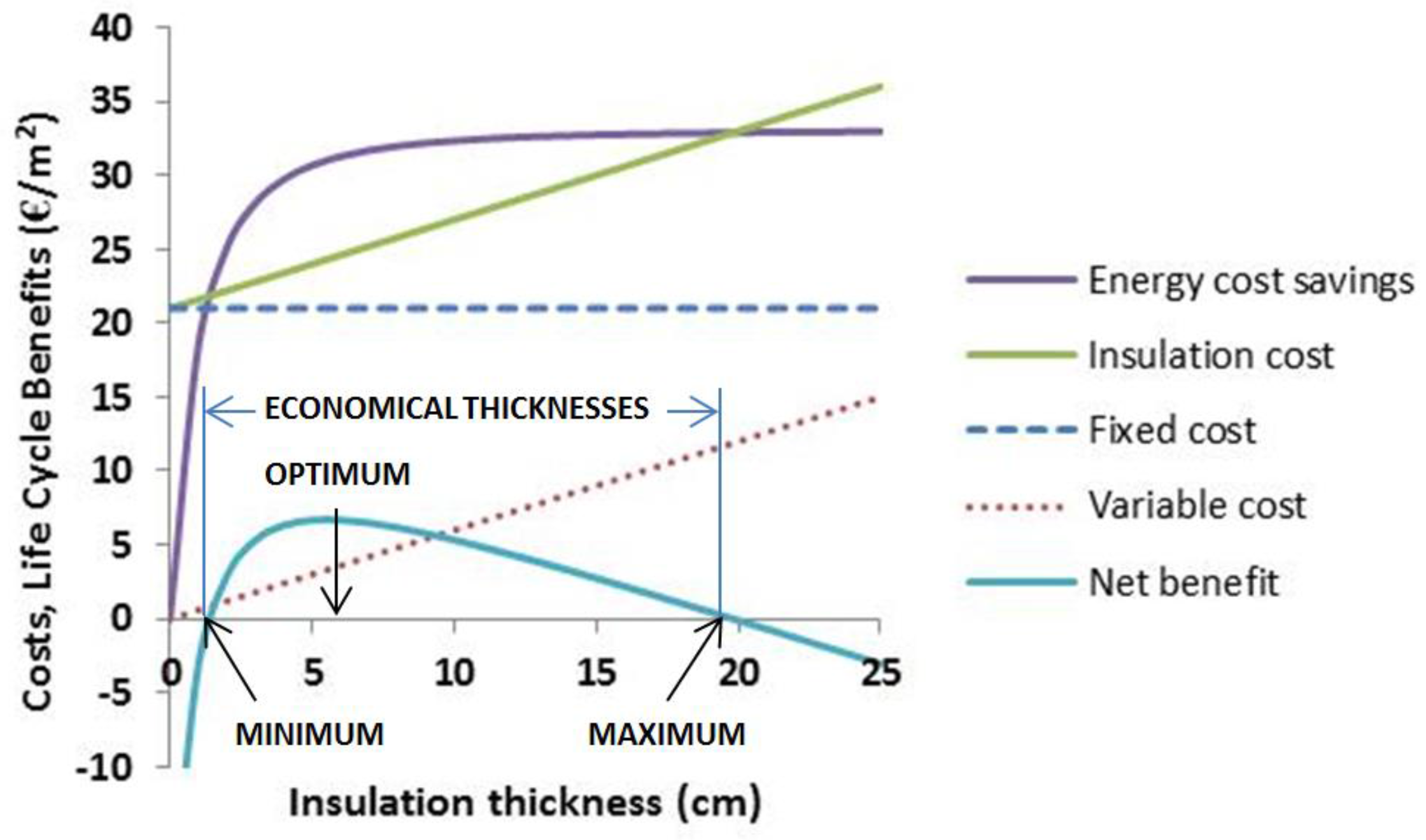For instance, in Greece, only half of the dwellings have some kind of envelope thermal insulation [4]. Some issues arise when retrofitting for insulation, with the principal being: the exact placement of the insulation (outside, inside, in cavity), the selection of insulation material and the required thickness for the insulating layer, with the last two interfering with each other. Insulation at buildings’ envelopes is regarded considering cost-effectiveness, as we observe a critical thickness after which the achievable energy cost savings do not pay back the further increment in insulation cost. In this sense, an optimum (and at the same time, economically maximum) insulation thickness (OIT) is introduced.

Optimum insulation thickness can be the outcome of detailed simulation [5]. Simplified analytical relations have also been proposed to the same aim, allowing the extraction of more general results, with limited accuracy however, as imposed by mathematical simplicity requirements. A great number of works on the determination of OIT have been elaborated in the past. An extended review on this topic is given in [6] and is not repeated here for economy of space. The problem of finding OIT is coped with the minimization of life cycle heating (and/or cooling) costs needed to compensate for the heat losses (and/or gains) through the considered fabric element. Both energy (fuel) and capital (insulation cost) expenses are accounted for and the issue renders to a single-objective optimization problem (minimization of the net present value of global costs):

$$Minimize\left\{\left(Annualheating/coolingcosts\right)·PWF\left(N,r\right)+\left(Insulationcost\right)\right\}$$

(1)

where $PWF(N,r)=[{(1+r)}^N-1]/[{(1+r)}^N·r]$ is the present worth factor for an N years’ constant annual cash flow and a discount rate of r.

Based on the above criterion, the researchers follow one of two distinguished alternative methods to find OIT, the first being a detailed simulation and the second an analytical relation based on simplification of the degree-days method. The application of detailed simulation leads to more accurate results by considering the effect of many factors. Nevertheless, the arising conclusions are site and case specific and, for this reason, of limited value to the designers/engineers. On the other hand, the proposed analytical relation ignores important factors, such as the effect of the insulation on the base temperature of the heated space and in this context it is set here under questionable accuracy.

Several researchers applied degree-days [7,8,9,10] and concluded to the same simple and explicit relation for the OIT_H (the subscript _H denotes the assumption of heating operation only):

$$OI{T}_H=293.94·\sqrt{\frac{D{D}_H·C_F·PWF·k_{INS}}{H_U·C_{INS}·n_{HS}}}-R_W·k_{INS}$$

(2)

where DD_H are the heating degree-days, C_F the cost of fuel, H_U its calorific value, n_HS the efficiency of the heating system, k_INS the thermal conductivity of the insulation material, C_INS the cost of insulation and R_W the initial thermal resistance of the wall (coefficient 293.94 stands for conversion of Watt-days to Joule).

On the other hand, Kayfeci et al. [11] found that the optimum insulation thickness may also depend on the cooling degree-days DD_C and the coefficient of performance of the cooling equipment COP. In the same context, Bolatturk [12] proposed two alternative values for OIT one for the heating and one for the cooling operation, while Kurekci [13] proposed furthermore an OIT_Y considering an all year around operation. In the same framework, a general relation to estimate OIT_Y, through considering both the heating and cooling energy needs, was proposed [13,14,15]:

$$OI{T}_Y=293.94·\sqrt{\frac{PWF·k_{INS}}{C_{INS}}·\left\{\frac{C_E·D{D}_C}{COP}+\frac{D{D}_H·C_F}{H_U·n_{HS}}\right\}}-R_W·k_{INS}$$

(3)

where C_E is the cost of electricity.

Although very simple and fast in estimating OIT, the degree-days concept and the subsequent simplified relations, Equations (2) and (3), have been criticized for inconvenience, by ignoring the effect of solar radiation and thermal mass [15,16]. Actually, there are a few other parameters that have also been confirmed as affecting OIT significantly, but are not included yet in the above relations. For instance, wall orientation was found to affect OIT by 0.5 cm for cold climates like the one in Elazig, Turkey (2653 heating degree-days) [17] up to 1.6 cm in warmer climates such as in Tunis (550 heating degree-days) [15]. Yuan et al. [18] investigated the optimum combination of external surface reflectivity and insulation thickness for several cities all over Japan thus demonstrating the effect of reflectivity on OIT. Other researchers examined alternatively the effect of external surface absorptance [17] and color [18] on OIT. In [16] it was examined the effect of shading on OIT, and demonstrated that full shading may decrease OIT by 3–3.5 cm (for a solar absorptance of 0.6). The significant effect of indoor temperature on OIT was also demonstrated [15], with the latter increasing remarkably with the winter base temperature. Other researchers investigated the effect of glazing area on OIT [19]; although they found that this does primarily affect the thermal load and consequently the achievable energy savings, it has a smaller effect on OIT which however can still reach up to 10% for the warmer areas of Turkey (region 1 of the Country’s climatic zones). For any of the above reasons, the proposed simplified analytical relations may prove inaccurate, when comparing their results to more accurately calculated OIT by using, for instance, Complex Finite Fourier Transform [15]. In this context, the need for amending the above relations, by incorporating additional parameters that proved to be of similar importance, arises.

In the previous publications on OIT, the optimization problem is regularly considered as an isolated one, focusing on the fabric element, and thus ignoring other data of the heated space which this element belongs to, such as the thermal transmittance of its other elements, the heat and the solar gains of the space, the thermal capacitance of the space etc. Only relatively recently, researchers took into consideration other data of the heated space [19]. As a consequence they found that insulation is more effective (energy savings are larger and payback period is shorter, for the same insulation thickness) in buildings with smaller window areas. In their calculations they assumed a monthly time step and a utilization factor for the gains. More specifically, they investigated the effects of an alteration of the glazing percentage from 10% to 50% of the wall area and indicated that optimum insulation thickness varies between 0.036 and 0.087 m (for extruded polystyrene foam and use of natural gas). In this way they indicated that OIT should not be examined by considering the fabric element alone, but through considering the integration of the latter to the heated space as well, without however concluding to any mathematical expression.

Although having indicated the dependence of OIT on characteristics of the heated space, the above researchers have not concluded to any relations that could be used as a guide to this aim. A comprehensive parametric analysis has been elaborated to this aim [20] but it was entirely based on Equation (3) ignoring in this context other parameters of the heated space that also affect OIT. In the present work we exactly assume thermal insulation of a fabric element as a more generalized issue, by considering it as an interfering with the heated space element. As a consequence, we investigate the effects of factors not included within the previously suggested relations, like the total heat losses coefficient of the space, the heat gains and all relevant parameters affecting these quantities. To keep our approach simple and broadly applicable, we also attempt to solve the problem analytically.

2. Methodology

2.1. Presentation of the Problem

The suggested analytical expressions Equations (2) and (3) include the heating degree-days which are usually calculated on a typical basis, e.g., for heating at 18 °C or 15.5 °C (used in the United Kingdom), or 65 °F (used in the United States) etc. [21]. The base temperature of a building may vary from month to month, but it is satisfactorily accurate to neglect this variation and assume a mean base temperature for the whole winter period (this is indicated later in the text, in Section 5.1) performing the calculations on the basis of the heating season (as also foreseen, among others, in EN ISO 13790). Emphasis is given on climates where heating degree-days exceed cooling degree-days and heating is the major concern, as it happened, for instance, with all European Countries.

By adding insulation to a fabric element, the total heat losses coefficient of the heated space do also change and consequently the same follows suit with the base temperature of the space. The greater the gains are, the more significant the effect is, as is indicatively shown in Figure 1. The figure is based on detailed simulation results through using TRNSYS, regarding a 100 m² apartment in Athens, Greece. From the figure it becomes apparent that insulation does not play any role in the balance temperature only when there are no heat gains. In contrast, the existence of gains results in a lower base temperature (the performance curve is shifted downwards). Moreover, the addition of insulation does also reduce further the base temperature (provided there are heat gains). The degree-days method offers a mathematical explanation for this behavior [22]. Anyway, the effect of the gains on the base temperature should be accounted for, when determining the optimum insulation thickness.

2.2. General Remarks

An analytical approach is followed here, in an attempt to conclude on more general results. To this aim, the degree-days method is also applied, and analytical relations are used (although approximate) e.g., for the heat gains utilization factor and for the heating degree-days. Although introducing some errors, these approximations have a minor impact on the determination of OIT due to the discrete thicknesses at which the insulation slabs are available. For instance, in Greece the respective thicknesses are 3, 5, 6, 7, 8, 10 and 12 cm; hence, an error smaller than ±5% seems acceptable, since within one standard error (68% probability in normal distribution [23]) do not fall more than one insulation thicknesses.

There are parameters which seem to have a minor effect on OIT. A sensitivity analysis will demonstrate whether these secondary parameters should also be taken into consideration in the optimization or not. We apply design of experiments [24], factorial simulation and analysis of variance (ANOVA), as it was similarly applied for envelope optimization in Malawi [25].

We assume the insulation of an opaque wall as a fabric element of a heated space where the latter generally constitutes part of a broader heated zone. Provided that the temperature distribution within the heat zone is uniform, no heat exchange takes place between the considered heated space and the rest of the zone. This is anyway desirable, to avoid overheating and thermal discomfort within the same heat zone, and can be easily attained (e.g., when heating is applied with radiators, by installing a thermostatic radiator valve (TRV) at each one of the heating elements and so on).

2.3. Consideration Regarding Insulation Costs

Fixed and variable costs are distinguished, when applying insulation slabs in retrofits. Fixed costs include the facilities for doing the job and the cost of placing the insulating panels on the wall, which are practically independent of the slab thickness. Insulation is placed preferably at the external side of the wall, hence the need to erect scaffolding; in addition, some materials are needed to secure installation and a decorative finishing touch (coat mesh, primer coat, render coat etc.). The space that is finally occupied by external insulation is not included in the built surface, a fact due to which there are no side costs (e.g., there is no loss of saleable floor area [26]). Labor costs and material costs to fix the wall insulation should be considered additional to the insulating slabs costs. All this however is not proportional to the volume (or equivalent to the thickness) of the insulation material, as is indicatively depicted for EPS in Figure 2. From this figure it becomes apparent that insulation material constitutes only a small part of the total cost, which is distinguished to a fixed and variable cost. Insulation material falls into the variable costs, together with the mechanical fixings, while all other components constitute the fixed costs. The total insulation costs (C_INS,TOT in €/m² of insulated surface) get consequently the form:

$$C_{INS,TOT}=C_{F,INS}+C_{V,INS}·X_{INS}$$

(4)

where X_INS is the insulation thickness (in m) and C_F,INS, C_V,INS are regression parameters (e.g., C_F,INS = 21 €/m² and C_V,INS = 60 €/m³). Although parameter C_F,INS has no effect in optimization, it becomes the critical one when evaluating the economy of the retrofit. Indeed, even for a wide layer of insulation (e.g., 10 cm thickness) the fixed expenses have the greatest share in the costs (almost 75% of total cost, correspondingly).

2.4. The Optimization Criterion

The usually applied criterion is the minimization of life cycle costs (see Equation (1)), and the optimization is applied based on the Life Cycle Cost Analysis LCCA [6]. The optimization can alternatively be based on the marginal quantities of the insulation cost and the induced energy cost savings. The maximum insulation thickness which is economical to reach, is when the marginal benefits (energy costs savings) cannot counterbalance any longer the marginal cost imposed by the addition of more insulation. In this sense, optimum insulation thickness arises when the derivative of the accumulated benefits get equalized to the derivative of the insulation cost.

Actually, in retrofits where fixed and variable insulation costs are distinguished, a minimum insulation thickness that can pay back the fixed expenses and its own cost comes first (Figure 3). Well after that comes a maximum insulation thickness which is the economically optimum (e.g., greater IRR) and at the same time the thickness beyond which any addition of insulation is not paid back from the respective achievable savings.

3. Commentary on the Most Important Factors that Affect Optimum Insulation Thickness

Optimum insulation thickness is a function of the building type, shape, orientation, construction materials, climatic conditions, insulation material and cost, energy type and cost, and the type and efficiency of air-conditioning system. Some of these factors are shortly commented below.

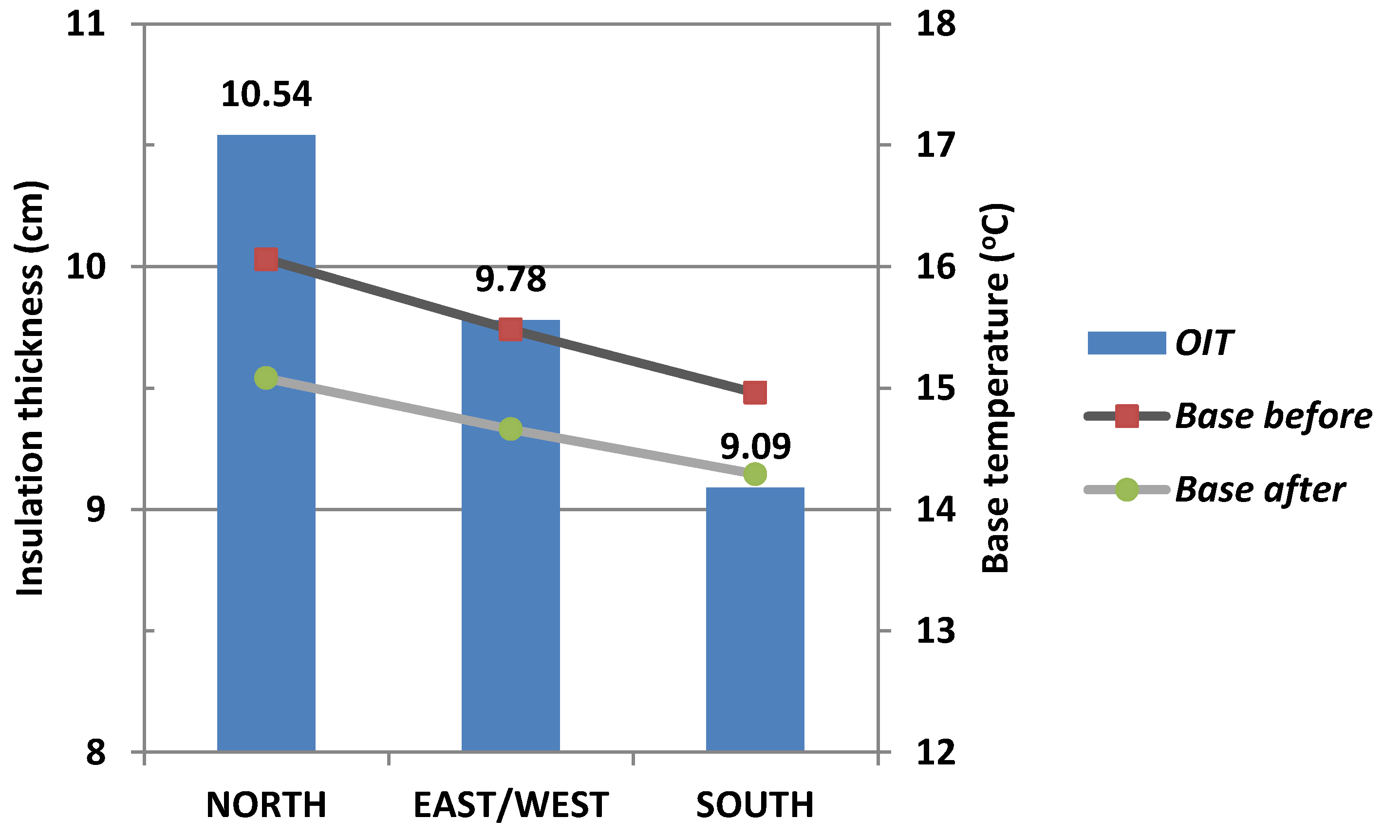
Heating degree-days: This is obviously the most important factor. High value of heating degree-days leads to greater achievable energy cost savings by applying insulation, and in this sense it is worth adding thicker layers of insulation. As a consequence, higher value of heating degree-days is reasonably expected to result in a greater optimum insulation thickness.

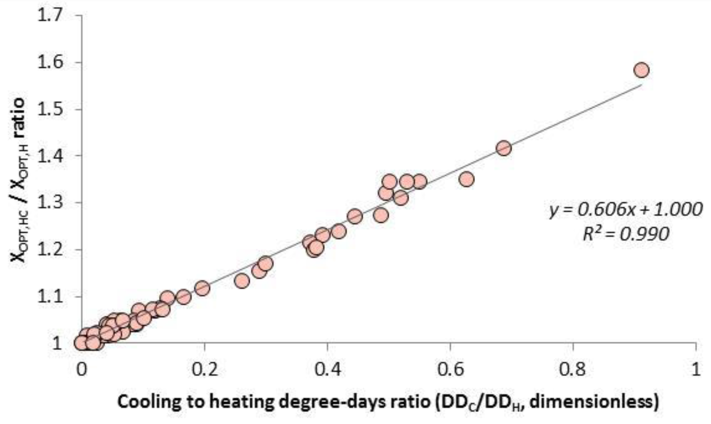
Cooling degree-days: The DD_C also affect optimum insulation thickness. In colder climates the OIT_H for heating does not significantly differ from the value OIT_Y regarding the heating and cooling operation, as it is depicted in Figure 4, which is based on published data [13]. A linear relation between these quantities: $\left(OI{T}_Y/OI{T}_H\right)=1.0+0.6·\left(CDD/HDD\right)$ is apparently valid The coefficient in front of the degree-days ratio (value 0.6) results from the division of costs for cooling and heating, correspondingly: $b=\left(C_E·H_U·n_{HS}\right)/\left(COP·C_F\right).$ Indeed, by introducing H_U = 34,485 kJ/m³, n = 0.90, C_F = 0.385 $/m³ from [12], C_E = 0.07 $/kWh [8] and COP = 2.5 [12,27] we estimate indeed b = 0.6. As a consequence, a more general relation may arise:

$$OI{T}_Y=OI{T}_H·\left(1+\frac{C_E}{COP}·\frac{H_U·n_{HS}}{C_F}·\frac{D{D}_C}{D{D}_H}\right)$$

(5)

An amended value of DD_C can be introduced in Equation (5), when adopting a different scenario of operation during the cooling period (e.g., unoccupied period due to summer holidays, intermittent operation etc.). For instance, in Greece it is assumed in the energy classification of buildings (based on ISO 13790) that the actual cooling energy needs are only 50% of the total cooling energy demand, hence the half value of DD_C should be respectively inserted in the above equation etc. thus causing a limited effect on OIT_Y. By taking into consideration that: (a) cooling degree-days affect OIT at a lesser degree than heating degree-days (b is generally much lower than unit) (b) for the weather conditions prevailing in the European Countries and more general in Countries with continental climates, heating accounts for a significant part of the total energy consumption (c) cooling load is only partly due to transmission gains through opaque surfaces (d) according to regulations, cooling may be considered covering part of the demand (e) optimum insulation thickness for year around operation can be easily extracted, by applying Equation (5) from optimum thickness for heating, we further consider in this work the determination of optimum insulation for heating operation only.

Existing insulation: The higher the existing insulation is, the lesser the room for further savings. Hence, preexistence of any insulation on the wall leads to a lower optimum insulation thickness. It is easily proved that the total insulation thickness should be anyway the same between pre-insulated and non-insulated walls, when pre-existing insulation (e.g., of thickness X_PI) is also accounted for in the total insulation thickness (provided that the same insulation material is considered). This is mathematically expressed by the relation:

$$OI{T}_H\left(X_{PI}=0\right)=OI{T}_H\left(X_{PI}\right)+X_{PI}$$

(6)

Such an issue is expected to arise when passing from already satisfactorily performing buildings to nearly zero energy buildings. Indeed, at an already insulated building, with X_PI, the X_OPT(X_PI) is expected to be much smaller and the question arising will be if it is worth proceeding with any additional insulation. In that case (but even more generally as well) the application of optimizing insulation thickness will not be enough but someone has to examine at first the profitability of the measure. If so, the fixed expenses should also be considered, and the following condition arises:

$$NPV=\left(Annualyavoidedenergycosts\right)·PWF\left(N,r\right)-\left(Insulationcost\right)>0$$

(7)

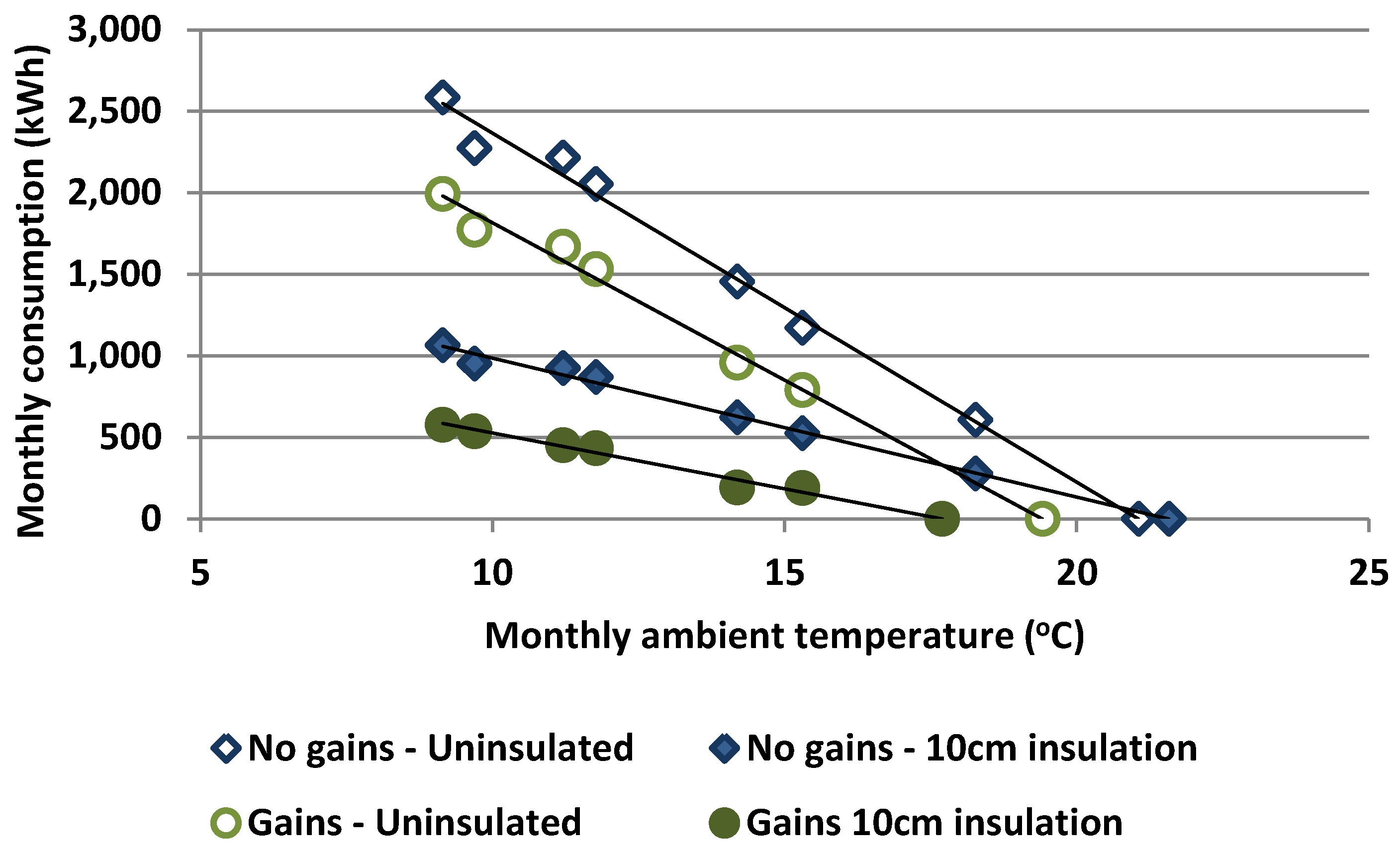
Heat and Solar gains: Heat and solar gains result in a lower base temperature, then in reduced heating degree-days, in lower energy needs and in the end in a smaller OIT_H value. The heat gains are more or less constant all through the year, while the solar gains vary. The application of insulation may reduce the solar gains through the opaque surface of the insulated wall, which constitutes however a minor part of solar gains in cases where the wall has some glazing surface on it.

Intermittency of operation: Intermittent heating is probably the rule in space heating. A night set-back temperature, and application of heating during occupancy hours only, lead to a lower mean temperature in the heated space and consequently to a reduced heating energy demand. The last fact has an impact on the economy of insulating, and reduces the OIT_H, since the achievable energy cost savings in intermittent heating operation (for the same insulation thicknesses) will be less. At the same time, however, the mean internal temperature is also reduced, in a way probably affecting the thermal comfort of the occupants. A compromise is finally desirable between the insulation cost and the thermal comfort, but such an approach is beyond the scope of the present work, where continuous heating is the main consideration.

Absorptance: The solar radiation incident on the external surface of the fabric element affects heat exchange with the environment. This is expressed via the sol-air temperature, which is strongly related to the absorptance and emittance of the surface:

$$T_{SOL-AIR}=T_A+\frac{F·I_T·a_{ES}}{h_{ES}}-\frac{{\epsilon }_{ES}·\Delta R}{h_{ES}}$$

(8)

where T_A is the outdoor air temperature (°C), F is the shading reduction factor for external obstacles on the surface, α_ES is the solar absorptance of the external surface, I_T is total solar irradiance incident on the surface (W/m²), h_ES is the combined convective and radiative heat transfer coefficient on the external surface (W/m² K), ε_ES is the hemispherical emittance of the surface and ΔR is the difference between the long-wave radiation incident on the surface from the sky and surroundings and the radiation emitted by a blackbody at outdoor air temperature (W/m²). The value of ΔR can be considered zero for vertical surfaces, because the radiant heat loss to the sky compensates the heat. Hence, solar gains through the opaque surface A* are equivalently expressed by the relation:

$$Q_S=A^{\ast }·\frac{F·I_T·a_{ES}}{h_{ES}}·U^{\ast }$$

(9)

where U* is the thermal transmittance of the considered fabric element. The higher the absorptance is, the higher the solar gains get, leading to respectively lower heating energy needs and in turn to lower values for OIT_H.

Economic factors: We distinguish cost factors (cost of insulation, cost of fuel) and financial factors (discount rate, life-time). All quantities are expressed in present values. The application of any loan can also be easily accounted for by converting all future installments on the debt to present values and adding them to the insulation cost.

The fact that the issue of specifying a suitable insulation thickness is multi-parametric arises as a conclusion of the above analysis of the factors affecting OIT. In addition, the wall should not be considered as isolated but as a constituent of the whole heated space.

4. Mathematical Background and Analytical Determination of the Optimum Insulation Thickness OIT_H

4.1. Formulation of the Problem

According to the criterion set in Section 2.4, OIT_H will result as the solution of the equalization between marginal benefits and marginal costs. Based on Equation (4), the annuity of the induced cost by implementing a differential thickness of insulation dX_INS is expressed, in present values, as:

$$d{C}_{TOT}=\frac{C_{V,INS}·A^{\ast }·d{X}_{INS}}{PWF\left(N,r\right)}$$

(10)

where N is the expected life time of insulation and r the discount rate. The annual benefits are respectively given by the relation:

$$d{B}_{TOT}=\frac{C_F·d{E}_{H,D}}{n_{HS}}$$

(11)

The estimation of the respective decrement of energy heating demand is not so straightforward, and is calculated as follows. According to the degree-days method, the annual energy demand of the heated space is:

$$E_{H,D}=TLC·D{D}_H\left(T_B\right)$$

(12)

where DD_H(T_B) are estimated at the base (or balance) temperature T_B. The total heat loss coefficient TLC of the heated space is given by the relation:

$$TLC=\frac{1}{3}·N_{AIR}·V+{\displaystyle \sum }_i\left(U_i·A_i\right)+U^{\ast }·A^{\ast }$$

(13)

where V is the volume of the heated space and N_AIR the infiltration rate through the space, expressed in air changes per hour; U_i is the thermal transmittance and A_i the respective surface area of any other external fabric element i of the considered space.

The fabric element for insulation is separately considered (not included in the summation term), unlike all other opaque surfaces of the heated space and openings which are included in the summation term. In the infiltration losses, only aeration through the openings between the space and the environment is considered. Aeration between the space under consideration and the other spaces of the zone do not contribute to the heating demand as long as the same internal temperature is sustained. The base temperature T_B is given by the relation:

$$T_B=T_{SP}-\frac{n_G·Q_G}{TLC}$$

(14)

where T_SP is the set-point temperature, Q_G the mean heat gains during the heating period and n_G the gains utilization factor. The addition of insulation decreases the thermal transmittance of the considered element and, according to Equation (9), the same takes place with the respective solar gains through this opaque surface. As a consequence, the heat gains are distinguished regarding their variation with insulation to (i) the variable ones like the solar gains through the opaque surface which is considered for insulation Q_GS^* and (ii) the fixed ones Q_GF which consist of the internal gains Q_GI and the solar gains through any glazing and any other opaque surfaces of the space Q_GS:

$$Q_G=Q_{GI}+G_{GS}+Q_{GS}^{\ast }=Q_{GF}+Q_{GS}^{\ast }$$

(15)

The differential of the annual energy demand is consequently:

$$d{E}_{H,D}=D{D}_H\left(T_B\right)·dTLC+TLC·D{D^{\prime }}_H\left(T_B\right)·d{T}_B$$

(16)

where $D{D^{\prime }}_H\left(T_B\right)$ is the derivative of heating degree-days:

$$D{D^{\prime }}_H\left(T_B\right)=\frac{d\left[D{D}_H\left(T_B\right)\right]}{d{T}_B}$$

(17)

By applying differentials in Equation (14) arises:

$$d{T}_B=-\left(\frac{Q_G}{TLC}\right)·d{n}_G-n_G·d\left(\frac{Q_G}{TLC}\right)$$

(18)

For continuous heating, the heat gains utilization factor is given by the relation:

$$n_G=\frac{1-{\gamma }^{\alpha }}{1-{\gamma }^{\alpha +1}}$$

(19)

with γ = Q_L/Q_G and α = 1 + τ/15, where τ is the time constant (in hours). A regression relation that gives the best fit to the utilization factor is [28]:

$$n_G=1-exp\left\{\frac{-k_G}{\raisebox{1ex}{$Q_G$}\!\left/ \!\raisebox{-1ex}{$Q_L$}\right.-D}\right\}$$

(20)

with k_G and D the regression parameters. According to a more recent study [29], parameter D ranges between (−0.02) and (−0.04) and in this sense is negligible within the accuracy limits of the present work. Parameter k_G is given as a function of the thermal capacity per floor area practically ranging between 1.0 and 1.2 for typical constructions with time constants 10 and 20 h, but also for heavy constructions (see Figure 5) as long as ratio γ becomes large (this is expected with the addition of insulation). Setting D ≈ 0, Equation (20) gets the form:

$$n_G=1-exp\left\{-k_G·\frac{Q_L}{Q_G}\right\}$$

(21)

It is also valid:

$$TLC=TL{C}_O+A^{\ast }·\left(U^{\ast }-U_O^{\ast }\right)$$

(22)

$$d\left(TLC\right)=A^{\ast }·d{U}^{\ast }$$

(23)

$$Q_L=Q_{LO}·\frac{TLC}{TL{C}_O}$$

(24)

where with index o the values of quantities U* and TLC before the application of insulation at the considered fabric element are denoted.

By using the above relations and applying simple algebra, the following relations arise:

$$d{n}_G=k_G·\left(1-n_G\right)·\frac{U_O^{\ast }·Q_{LO}}{TL{C}_O}·\frac{Q_{GF}·U_O^{\ast }·A^{\ast }-\left(TL{C}_O-U_O^{\ast }·A^{\ast }\right)·Q_{GSO}^{\ast }}{{\left(U_O^{\ast }·Q_{GF}+Q_{GSO}^{\ast }·U^{\ast }\right)}^2}·d{U}^{\ast }$$

(25)

$$d\left(\frac{Q_G}{TLC}\right)=\frac{TL{C}_O·Q_{GSO}^{\ast }-A^{\ast }·U_O^{\ast }·\left(Q_{GF}+Q_{GSO}^{\ast }\right)}{U_O^{\ast }·{\left\{TL{C}_O+A^{\ast }·\left(U^{\ast }-U_O^{\ast }\right)\right\}}^2}·d{U}^{\ast }$$

(26)

$$d{T}_B=\left[-\frac{k_G·\left(1-n_G\right)·Q_{LO}}{TL{C}_O}·\frac{Q_{GF}·U_O^{\ast }·A^{\ast }-\left(TL{C}_O-U_O^{\ast }·A^{\ast }\right)·Q_{GSO}^{\ast }}{U_O^{\ast }·Q_{GF}+Q_{GSO}^{\ast }·U^{\ast }}-\frac{n_G}{TLC}·\left\{\frac{TL{C}_O}{U_O^{\ast }}·Q_{GSO}^{\ast }-A^{\ast }·\left(Q_{GF}+Q_{GSO}^{\ast }\right)\right\}\right]·\frac{1}{TLC}·d{U}^{\ast }$$

(27)

$$d{E}_{H,D}\approx A^{\ast }·D{D}_H\left[T_{SP}-\frac{n_G·Q_{GSO}^{\ast }}{A^{\ast }·U_O^{\ast }}-\frac{k_G·\left(1-n_G\right)·Q_{LO}}{TL{C}_O·A^{\ast }}·\frac{Q_{GF}·U_O^{\ast }·A^{\ast }-\left(TL{C}_O-U_O^{\ast }·A^{\ast }\right)·Q_{GSO}^{\ast }}{U_O^{\ast }·Q_{GF}+Q_{GSO}^{\ast }·U^{\ast }}\right]·d{U}^{\ast }$$

(28)

The addition of insulation decreases the thermal transmittance of the element, according to the relation:

$$U^{\ast }=\frac{1}{\raisebox{1ex}{$1$}\!\left/ \!\raisebox{-1ex}{$U_O^{\ast }$}\right.+\raisebox{1ex}{$X_{INS}$}\!\left/ \!\raisebox{-1ex}{$k_{INS}$}\right.}$$

(29)

The differential of U* becomes:

$$d{U}^{\ast }=-\frac{d{X}_{INS}}{k_{INS}·{\left(\raisebox{1ex}{$1$}\!\left/ \!\raisebox{-1ex}{$U_O^{\ast }$}\right.+\raisebox{1ex}{$X_{INS}$}\!\left/ \!\raisebox{-1ex}{$k_{INS}$}\right.\right)}^2}=-\frac{U^{\ast 2}·d{X}_{INS}}{k_{INS}}$$

(30)

Heating degree-days can be quite accurately written as a quadratic function of the base temperature [30]:

$$D{D}_H\left(T_B\right)\approx A_{DD}·{\left(T_B-T_{MIN}\right)}^2$$

(31)

with

$$T_{MIN}=T_{REF}-\frac{2·D{D}_H\left(T_{REF}\right)}{N_Y}·\left\{1+\sqrt{1-\frac{N_Y·\left(T_{REF}-T_{MEAN}\right)}{D{D}_H\left(T_{REF}\right)}}\right\}$$

(32)

and

$$A_{DD}=\raisebox{1ex}{$91.25$}\!\left/ \!\raisebox{-1ex}{$\left(T_{MEAN}-T_{MIN}\right)$}\right.$$

(33)

Here, T_REF is the reference temperature used as the basis for the calculation of heating degree-days DD_H(T_REF) and T_MEAN the mean annual temperature of the site.

By introducing the above second degree approximation in heating degree-days for the estimation of dE_H,D in Equation (28), and by equalizing marginal costs and marginal benefits (dC_TOT = dB_TOT), the following implicit equation of U^* finally arises:

$$\begin{array}{cc}F\left(U^{\ast }\right)=& \{T_{SP}-T_{MIN}-\frac{n_G·Q_{GSO}^{\ast }}{A^{\ast }·U_O^{\ast }}-\frac{k_G·(1-n_G)·Q_{LO}}{A^{\ast }·TL{C}_O}\\ & ·\frac{Q_{GF}·U_O^{\ast }·A^{\ast }-(TL{C}_O-A^{\ast }·U_O^{\ast })·Q_{GSO}^{\ast }}{U_O^{\ast }·Q_{GF}+Q_{GSO}^{\ast }·U^{\ast }}\}·U^{\ast }\\ & -\sqrt{\frac{C_{V,INS}·n_{HS}·k_{INS}}{0.024·A_{DD}·PWF(N,r)·C_F}}=0\end{array}$$

(34)

Coefficient 0.024 is introduced to convert W-days to kWh, assuming that the fuel cost is expressed per kWh of fuel calorific value. Here, n_G is also a function of U^*:

$$n_G=1-exp\left\{-k_G·\frac{Q_{LO}·\frac{TL{C}_O+A^{\ast }·\left(U^{\ast }-U_O^{\ast }\right)}{TL{C}_O}}{Q_{GF}+Q_{GSO}^{\ast }·\raisebox{1ex}{$U^{\ast }$}\!\left/ \!\raisebox{-1ex}{$U_O^{\ast }$}\right.}\right\}$$

(35)

The last set of equations, Equations (34) and (35), constitutes an implicit system of equations for the estimation of the optimum thermal transmittance U* that corresponds to the OIT_H.

4.2. Solution of the Implicit Set of Equations

4.2.1. Application of a Trial and Error Process

The accurate solution of the implicit set of Equations (34) and (35) is of low practical value for rigid insulating slabs, as they are available at discrete thicknesses. Equation (34) has resulted by subtracting insulation costs from energy cost savings, and for this reason a positive value of F(U^*) does precisely mean that the benefits by insulating exceed the respective costs. In this way, the various available insulation slab thicknesses can be tried, and the greater one that still results in a positive value for F(U*) can finally be selected.

4.2.2. Successive Substitution

Equation (34) can be solved for U* to get the form:

$$U^{\ast }=\frac{\sqrt{\frac{C_{V,INS}·n_{HS}·k_{INS}}{0.024·A_{DD}·PWF\left(N,r\right)·C_F}}}{\left\{T_{SP}-T_{MIN}-\frac{n_G·Q_{GSO}^{\ast }}{A^{\ast }·U_O^{\ast }}-\frac{k_G·\left(1-n_G\right)·Q_{LO}}{A^{\ast }·TL{C}_O}·\frac{Q_{GF}·U_O^{\ast }·A^{\ast }-\left(TL{C}_O-A^{\ast }·U_O^{\ast }\right)·Q_{GSO}^{\ast }}{U_O^{\ast }·Q_{GF}+Q_{GSO}^{\ast }·U^{\ast }}\right\}}$$

(36)

By setting initial value of U* = U₀*, and introducing it consecutively to Equation (35) and to the right side of Equation (36), a new U* arises to the left side of Equation (36); this is also inserted in Equation (35) and to the right side of Equation (36) and so on. By these consecutive substitutions, convergence to the optimum value of U* is rapidly achieved (practically, two to three successive substitutions are sufficient). The whole approach is indicatively depicted in Figure 6.

4.2.3. Use of a Solver

The implicit set of Equations (34) and (35) can easily be solved by any solver like Mathematica or Maple (the latter is also integrated within MATLAB). Alternatively, the Excel software package (and its add-in solver) can also be used.

4.2.4. Approximate Graphical and Analytical Solutions

Graphical Solution

Solar gains, through the opaque surface of the considered fabric element are expected to constitute a minor part of total gains. For this reason, their variation with the thermal transmittance of the element can be ignored, without introducing a significant error. Then, the gains Q_GS^* are included in the fixed gains:

$$Q_{GF}\cong Q_{GI}+G_{GS}+Q_{GSO}^{\ast }when{Q}_{GS}^{\ast }~constant$$

(37)

By removing Q_GSO^* from Equations (34) and (35), they get the following simpler forms:

$$\left\{T_{SP}-T_{MIN}-\frac{k_G·\left(1-n_G\right)·Q_{LO}}{TL{C}_O}\right\}·U^{\ast }-\sqrt{\frac{C_{V,INS}·n_{HS}·k_{INS}}{0.024·A_{DD}·PWF\left(N,r\right)·C_F}}=0$$

(38)

$$n_G=1-exp\left\{-\frac{k_G·Q_{LO}}{Q_{GF}·TL{C}_O}·\left[TL{C}_O+A^{\ast }·\left(U^{\ast }-U_O^{\ast }\right)\right]\right\}$$

(39)

Setting:

$$z=\frac{k_G·Q_{Lo}·A^{\ast }·U^{\ast }}{Q_{GF}·TL{C}_O}$$

(40)

$$a=\frac{k_G·Q_{Lo}}{TL{C}_O·\left(T_{SP}-T_{MIN}\right)}·exp\left[-\frac{k_G·Q_{Lo}}{Q_{GF}·TL{C}_O}·\left(TL{C}_O-A^{\ast }·U_O^{\ast }\right)\right]$$

(41)

$$b=\frac{k_G·Q_{Lo}·A^{\ast }}{Q_{GF}·TL{C}_O·\left(T_{SP}-T_{MIN}\right)}·\sqrt{\frac{C_{V,INS}·n_{HS}·k_{INS}}{0.024·A_{DD}·PWF\left(N,r\right)·C_F}}$$

(42)

the system of equations (38) and (39) renders to a single equation of z:

$$e^z=\frac{a·z}{z-b}$$

(43)

or equivalently to:

$$\left(z-b\right)·e^{z-b}=a·z·e^{-b}$$

(44)

By applying the Lambert function W to both parts of Equation (44) (the Lambert function is defined as the inverse relation of the function F(z) = z·e^z) we get:

$$z-b=W\left(a·z·e^{-b}\right)$$

(45)

At last, by transforming z:

$$z^{\prime }=a·z·e^{-b}$$

(46)

the Equation (45) gets the final form:

$$z^{\prime }·\frac{e^b}{a}-b=W\left(z^{\prime }\right)$$

(47)

Equation (47) can be solved graphically in a diagram of Lambert function, or by using the discrete values of Lambert function given in

Table 1. Values of Lambert W function.

z	W(z)	z	W(z)	z	W(z)	z	W(z)
0.001	0.001	0.01	0.0099	0.1	0.0913	1.5	0.7259
0.002	0.002	0.02	0.0196	0.2	0.1689	2.0	0.8526
0.003	0.003	0.03	0.0291	0.3	0.2368	2.5	0.9586
0.004	0.004	0.04	0.0385	0.4	0.2972	3.0	1.0499
0.005	0.005	0.05	0.0477	0.5	0.3517	3.5	1.1303
0.006	0.006	0.06	0.0567	0.6	0.4016	4.0	1.2022
0.007	0.007	0.07	0.0656	0.7	0.4475	4.5	1.2672
0.008	0.0079	0.08	0.0743	0.8	0.4901	5.0	1.3267
0.009	0.0089	0.09	0.0828	0.9	0.5298	5.5	1.3815
0.010	0.0099	0.10	0.0913	1.0	0.5671	6.0	1.4324

. After finding the root z’, we calculate z, then U* and finally the required OIT_H.

Analytical Solution

The set of Equations (38) and (39) can be solved analytically only when the variation of the base temperature with the addition of insulation is ignored. Then, the set is solvable for U*:

$$U^{\ast }=\frac{TL{C}_O·\sqrt{\frac{C_{V,INS}·n_{HS}·k_{INS}}{0.024·A_{DD}·PWF\left(N,r\right)·C_F}}}{TL{C}_O·\left(T_{SP}-T_{MIN}\right)-k_G·Q_{LO}·exp\left\{-\frac{k_G·Q_{LO}}{Q_{GF}}\right\}}$$

(48)

which, if solved for X_INS, becomes practically identical to the previously suggested Equation (3) where the base temperature is now corrected to the actual balance temperature of the heated space (just before the application of insulation).

5. Results and Discussion

5.1. Demonstrative Example

The present analytical approach is demonstrated through the following example. A heated space with dimensions of 5 × 5 × 3 m³ (W × L × H), having an external wall facing to the west which additionally includes a double-glazed window, is in thermal equilibrium with adjacent, above and below heated spaces (see Figure 7). The wall is assumed to be consisted of three successive layers, an internal plaster layer of 0.02 m, a brick layer of 0.18 m and an external plaster layer of 0.02 m. Assuming internal and external thermal resistances of 0.13 m²-K/W and 0.04 m²-K/W, respectively, the initial thermal transmittance of the wall is estimated at 1.613 W/m²-K.

The following are assumed for the calculation of internal gains. Population density 5 persons/100 m², installed power for lighting 3.6 W/m², use of lighting 6 h per day, sensible heat released 80 W/person, presence factor 0.75, installed capacity for equipment 4 W/m², intermittency factor 0.5. According to them, the 24 h mean internal gains are 135 W.

In

Table 2. Incident solar radiation (kWh/m²-mo) in Athens, on vertical surfaces with various orientations.

	NORTH	EAST/WEST	SOUTH
J	19	43	95
F	24	49	88
M	37	71	95
A	49	86	89
M	69	111	88
J	78	119	85
J	78	125	92
A	64	119	103
S	43	91	110
O	31	65	113
N	20	48	103
D	17	40	94

the incident solar radiation values for various wall orientations in Athens are presented. In

Table 3. Estimation of the duration of the heating period and the respective mean gains.

	Temperature (°C)	Solar Irradiance (W/m2)	Total Gains (W)	Heat Losses (W)	Utilization Factor of the Gains	Base Temperature (°C)
J	9.15	58	233	408	0.83	14.9
F	9.69	72	257	388	0.78	14.7
M	11.77	95	296	309	0.65	14.9
A	15.30	119	337	177	0.41	16.3
M	20.24	149	387	0	0.00	20.0
J	24.28	165	414	0	0.00	20.0
J	27.04	168	419	0	0.00	20.0
A	26.67	160	405	0	0.00	20.0
S	22.98	126	349	0	0.00	20.0
O	18.27	87	283	65	0.21	18.5
N	14.19	67	248	219	0.59	16.1
D	11.20	54	226	331	0.77	15.4
Mean values 1	12.80	79	268	271		15.8

¹ referring to the heating period (October to April).

the monthly temperatures and calculated mean solar irradiance on the west facing wall, the total gains (including internal gains, solar gains through glazing and through the opaque surface), the gains utilization factor and finally the base temperature for each month, are additionally depicted. In this sense, the months in which heating is necessary finally arise (the base temperature exceeds the monthly temperature).

The mean value of monthly base temperatures of the heating period (from October to April, here) is calculated at 15.8 °C. Alternatively, through using the mean quantities for heat losses and gains for the whole heating period (presented in the last line of the same table), the base temperature would have been estimated at 15.5 °C, which reveals that the use of mean data for the whole heating period introduces some error. This small error however is negligible as equally concerning both the previously suggested analytical relation and the analytical approach proposed here, since neither applies variable-base degree-days. The necessary data for the calculations are further presented in

Table 4. Data used in the example.

General Data of the Wall and the Heated Space	Values
Volume of the heated space	75 m3
Infiltration rate	0.25 ach
Floor area of the heated space	25 m2
Thermal construction	Light (kG = 1)
Efficiency of heating system	0.80
Area of the wall	15 m2
Orientation of the wall	West
Shading factor at the wall	0.9
Area of the window at the wall (20% glazing)	3 m2
U-value of the window at the wall	4.0 W/m2-K
Solar heat gain coefficient for the window	0.54
Net area of the wall to be insulated	12 m2
Initial thermal transmittance of the wall	1.613 W/m2-K
Absorptance of external surface	0.3
Convection/radiation coefficient for external surface	25 W/m2-K
Thermal conductivity of insulation	0.04 W/m-K
Weather Data	Values
Mean temperature at the area	17.61 °C
Reference temperature for the heating degree-days	18 °C
Heating degree-days at reference temperature	1225 K-days
Economic Data	Values
Life time	20 years
Discount rate	0.07
Cost of insulation material	60 €/m3
Cost of fuel	0.08 €/kWh

.

According to the weather data of Table 4, we estimate:

$$T_{MIN}=18-\frac{2\times 1225}{365}\times \left\{1+\sqrt{1-\frac{365\times \left(18-17.61\right)}{1225}}\right\}=4.98℃$$

(49)

$$A_{DD}=\raisebox{1ex}{$91.25$}\!\left/ \!\raisebox{-1ex}{$\left(17.61-4.98\right)$}\right.=7.225$$

(50)

In

Table 5. Calculated quantities in the demonstrative examples.

Initial total heat loss coefficient of the space	38 W/K
Mean ambient temperature at the heating period	12.8 °C
Initial mean losses in winter period	270.9 W
Mean incident radiation at the wall in the heating period	57.4 kWh/m2-mo
Mean gains in winter period	267.6 W
Fixed mean gains in winter period	251.2 W
Variable (with transmittance) solar gains in winter period	16.4 W

other input necessary for the application of the relations proposed here, which are also calculated from the data of Table 3 and Table 4 are presented. The application of the presented alternative methods to solve this problem is indicated below.

A. Solution by checking available thicknesses of insulating slabs

For each one of the available insulation thicknesses we calculate U* by using Equation (29), then n_G by using Equation (35) and last F(U*) by using Equation (34), as shown in

Table 6. Trial and error method to find optimum thermal transmittance U*.

XINS (m)	U*(W/m2-K)	F(U*)
0.03	0.730	4.775
0.05	0.535	2.429
0.06	0.472	1.686
0.07	0.422	1.104
0.08	0.382	0.637
0.10	0.321	−0.066
0.12	0.276	−0.570

. According to these trials, it seems that there is no benefit to reach a thickness of 0.10 m, hence a slab of 0.08 m seems a safe selection instead. Noticeably, F(U*) is slightly negative at 0.10 m, thus if slabs were available at continuous thicknesses, the optimum thickness would be a value closer to 0.10 than to 0.08 m.

B. By applying successive substitutions

Starting from the initial value of U_O* = 1.613 W/m²-K (for X_INS = 0) we rapidly conclude to the final value of OIT_H = 9.78 cm just after two consecutive substitutions, as indicated in

Table 7. Application of successive substitutions to find optimum thermal transmittance U*.

U* (W/m2-K)	nG	New U* (W/m2-K)	Respective XINS (m)
1.6130	0.639	0.2965	0.1107
0.2965	0.463	0.3273	0.0974
0.3273	0.469	0.3263	0.0978
0.3263	0.468	0.3263	0.0978

. It is noticed here that we could alternatively start from the thermal transmittance set by the regulations (e.g., 0.5 W/m²-K) to reach even faster the final solution.

C. By applying a solver

By applying the solver of MATLAB we estimate OIT_H = 9.7796676 cm. Hence, the 0.10 m slab is indeed marginally acceptable.

D. By applying a graphical solution

In this case, we include the solar gains through the opaque surface (8 W) to the fixed gains, and so total fixed gains reach the value of Q_GF = 268 W. We estimate:

$$a=\frac{1\times 271}{38\times \left(20-4.98\right)}\times exp\left[-\frac{1\times 271}{268\times 38}\times \left(38-12\times 1.613\right)\right]=0.2889$$

(51)

$$b=\frac{1\times 271\times 12}{268\times 38\times \left(20-4.98\right)}\times \sqrt{\frac{60\times 0.80\times 0.04}{0.024\times 7.225\times 10.594\times 0.08}}=0.0769$$

(52)

Then e^b/a = 3.7380, and the following equation arises:

$$3.7380·z^{\prime }-0.0769=W\left(z^{\prime }\right)$$

(53)

Which can be graphically solved (see Figure 8) to give the root z’ = 0.0278. Indeed, based on the figure we realize that the solution is between the z’ values 0.02 and 0.03. We apply linear interpolation to the data of Table 3, for z’ values 0.02 and 0.03: W(z’) = 0.95z’ + 0.006, and then by setting this equal to W(z’) = 3.7380z’ − 0.0769 we get z’ = (0.0769 + 0.0006)/(3.7380 − 0.95) = 0.0277977.

Then z = z’·e^b/a = 0.0278·3.7380 = 0.1039, and U^* is estimated:

$$U^{\ast }=z·\frac{Q_G·TL{C}_O}{k_G·Q_{Lo}·A^{\ast }}=0.1039\times \frac{268\times 38}{1\times 271\times 12}=0.3249$$

(54)

and the optimum insulation thickness:

$$OI{T}_H=k_{INS}·\left[\frac{1}{U^{\ast }}-\frac{1}{U_O^{\ast }}\right]=0.04\times \left[\frac{1}{0.3249}-\frac{1}{1.613}\right]=0.0983m$$

(55)

This graphical solution has an error of only 0.5% in comparison with the accurate solution attained through using a solver (0.0978 m).

E. By applying the analytical relation

By applying Equation (48) we calculate:

$$U^{\ast }=\frac{38\times \sqrt{\frac{60\times 0.80\times 0.04}{0.024\times 7.225\times 10.594\times 0.08}}}{38\times \left(20-4.98\right)-1.0\times 271\times exp\left\{-\frac{1.0\times 271}{268}\right\}}=0.3082W/\left(m^2·K\right)$$

(56)

which leads to the value OIT_H = 0.1050 m which has an error of 7.4% (comparably to the accurate value of 0.0978 m).

If a base temperature of 18 °C was used instead, then by using Equation (2) and introducing C_F/H_U = 0.08 €/kWh = 2.222·10⁻⁸ €/J, we would calculate:

$$OI{T}_H=293.94\times \sqrt{\frac{1225\times 2.222\times {10}^{-8}\times 10.594\times 0.04}{60\times 0.80}}-\frac{1}{1.613}\times 0.04=0.1193m$$

(57)

thus overestimating by +22% the optimum insulation thickness.

5.2. Effect of Orientation

All three alternative methods suggested (trial and error, successive substitution and graphical solution) lead quickly and satisfactorily to the optimum thermal transmittance calculated accurately with a solver (0.33 W/m²-K) and to the respective optimum insulation thickness (0.098 m).

The analytical relations instead, introduce a significant error (+22%) when a typical base temperature is used (e.g., 18 °C) which is reduced to 7.4% in this specific example, when the actual base temperature is applied.

The calculated OIT for Athens (9.8 cm) is in agreement with relevant published results of detailed simulation (e.g., an OIT of 8 cm was calculated for Iraklion—it is at the Southern part of Greece, heating degree-days 1056 K-days—in the frame of energy efficient nZEB design [31]). The respective optimum thermal transmittance U* = 0.33 W/m²-K is almost 35% lower than the corresponding maximum permitted value set by the Greek regulation for the assumed climatic zone (U_MAX = 0.50 W/m²-K).

The above assumed relations can be taken into consideration in relation to several parameters, such as the orientation which has been proved to be critical in OIT_Y determination [32] but not regarded in the analytical expressions Equations (2) and (3). Indeed, let’s assume that the wall has a due south orientation. The fixed gains and the variable solar gains are now 327.6 W and 27.6 W, respectively. Solving again as above, we find OIT_H = 9.093 cm.

Last but not least, by assuming the north orientation, we now estimate the same heating period (seven months) but the fixed gains and the variable solar gains arise at present to 191.1 W and 8.0 W, respectively. Solving again as above, we find OIT_H = 10.541 m. In this case, the installation of a 0.10 m insulating slab can be proposed.

The above estimations are depicted in Figure 9 together with the respective base temperatures, before and after the application of optimum insulation. It is firstly apparent that the assumption of a typical base temperature, such as 18 °C, is misleading as base temperatures are even 4 °C lower. Secondly, the effect of insulation on the base temperature which, for the assumed data, ranges from 0.7 to 1.0 °C also becomes apparent documenting once again the feasibility to take into consideration the base temperature variation when searching for the optimum insulation thickness.

5.3. Sensitivity Analysis

5.3.1. Revealing the Main Factors that Affect Optimum Insulation Thickness

Sensitivity analysis is further applied to the data and the results of the example, in discovering which are the most critical parameters affecting optimum insulation thickness in an area. To this aim, we vary (e.g., by ±20%) the main parameters of Equations (34) and (35). It is noticed that some of these quantities appear only in the form of a common factor, as is the case with the parameters under the square root of the equation, the effect of which is reasonably evaluated through the respective composite factor:

$$S=\frac{C_{V,INS}·n_{HS}·k_{INS}}{PWF\left(N,r\right)·C_F}$$

(58)

In this context, we vary the considered parameters within the ranges shown in

Table 8. Parameters considered in the sensitivity analysis and respective ranges of variation.

Parameter	Low Value	Reference Value	High Value
U-wall (W/m2-K)	1.29	1.61	1.93
U-window (W/m2-K)	3.20	4.00	4.80
Glazing (% of the wall area)	16.0	20.0	24.0
Heat gains (W/m2-floor area)	4.32	5.40	6.48
Incident solar radiation (W/m2)	62.76	78.45	94.14
SHGC (nd)	0.432	0.54	0.648
Absorptance (nd)	0.24	0.30	0.36
Infiltration rate (ach)	0.20	0.25	0.30
Factor-S (W2/m4)	10.45	13.06	15.68

and plot their effect on the optimum thermal transmittance in a normal probability diagram (Figure 10).

From Figure 10, the composite quantity S arises as the most important parameter. This is quite reasonable for an economic optimization issue, as it incorporates all financial parameters. The strong volatility of energy prices, as is indicatively shown for natural gas in Figure 11, and in turn the variability of factor S, should be noticed here however. In this sense, any proposals for OIT should be thoroughly considered, as long as life cycle savings are accounted for. For instance, the drop in the price of natural gas from 0.08 to 0.06 €/kWh-GCV results in a 33% increase in factor-S leading to 15% higher U^* value and finally to 16% smaller OIT_H (0.0819 m instead of 0.0978 m calculated earlier).

In addition, the heat gains, the incident solar radiation and the solar gain heat coefficient, have significant positive effects (on the optimum thermal transmittance). An increase of these factors leads to higher thermal transmittance values, or equivalently to lower values of economical insulation. On the other hand, the thermal transmittance of the window in the heated space and the infiltration rate through the space, have negative effects, as well. Both last parameters affect the total heat loss coefficient and in this sense their increase leads to lower thermal transmittance values. The glazing area seems to be effected neutrally. This is due to the fact that increased glazing leads to higher heat losses but at the same time to greater solar gains, which seem to counterbalance each other in this specific example.

The absorptance of the external surface of the wall does not seem to have a significant effect. The same is valid, regarding the initial value of the thermal transmittance of the wall. This last fact is very reasonable, meaning that the optimum total insulation thickness is independent of the initially placed insulation (see Equation (6) and relevant comments in Section 3).

The above results are also presented in the form of ANOVA, in

Table 9. Analysis of variance (ANOVA) for selected model for optimum U*.

Source	Sum of		Mean	F	p-Value
	Squares	df	Square	Value	Prob > F
Model	0.15	6	0.025	4279.26	<0.0001
B-U-window	5.863 × 10−3	1	5.863 × 10−3	992.57	<0.0001
D-Heat gains	6.069 × 10−3	1	6.069 × 10−3	1027.48	<0.0001
E-Solar radiation	5.346 × 10−3	1	5.346 × 10−3	905.10	<0.0001
F-SHGC	4.062 × 10−3	1	4.062 × 10−3	687.65	<0.0001
H-Infiltration rate	1.665 × 10−3	1	1.665 × 10−3	281.92	<0.0001
J-Factor-S	0.13	1	0.13	21780.82	<0.0001
Residual	7.206 × 10−4	122	5.907 × 10−6
Cor Total	0.15	128

(printout of Design Expert ver.10 code). The assumed model (including the parameters B = U-window, D = Heat gains, E = Solar radiation, F = SHGC, H = Infiltration rate, J = Factor-S) scores an F-value of 4279.26 which implies that the model is significant. Values of “Prob > F” less than 0.0500 indicate that model terms are significant. In this case, B, D, E, F, H, J are indeed significant model terms.

The resulting linear regression equation (with the parameters set in their coded values, ranging from −1 to +1), is:

$$\mathrm{Optimum}-{\mathrm{U}}^{\ast }=+0.3243-6.768\times {10}^{-3}·\mathrm{B}+6.886\times {10}^{-3}·\mathrm{D}+6.463\times {10}^{-3}·\mathrm{E}+5.633\times {10}^{-3}·\mathrm{F}-3.607\times {10}^{-3}·\mathrm{H}+0.0317·\mathrm{J}$$

(59)

From this equation it becomes apparent that factor S has almost five times greater an effect than each one of the others. On the other hand, all other parameters together (heat gains, incident solar radiation/orientation), solar heat gain coefficient, thermal transmittance of the window and infiltration rate) may cause an equally significant effect similar to the one of factor S. Indeed, the summation of the absolute values of the respective regression coefficients of parameters B, D, E. F and H equals 29.36 × 10⁻³ which is comparable to the coefficient of parameter J 31.70 × 10⁻³. For this reason, the effect of all these secondary parameters should not be neglected, when searching for the optimum insulation thickness.

5.3.2. Evaluating Divergences from the Previously Proposed Analytical Equation for OIT_H

In continuation to the above sensitivity analysis, we further calculate for all arising combinations of parameters the respective optimum insulation thickness (OIT_H). These values are now compared to those estimated by the analytical expressions of Equation (2), where the actual base temperature is correctly introduced (however as already explained, by applying a typical base temperature like 18 °C the results are misleading). The comparison is depicted in Figure 12. From the figure it becomes apparent that the previously suggested analytical expression (Equation (2)) always overestimates the required insulation by almost +12%, as a mean value. There are cases however where this overestimation reaches even 20% leading to a greater thickness by +2 cm and becoming in this way very significant, when the discretization of the available thicknesses for the insulating slabs (thickness step 1–2 cm) is taken into consideration.

The ANOVA for the divergences in OIT_H, is presented in

Table 10. Analysis of variance (ANOVA) of selected model for Delta(OIT_H).

Source	Sum of		Mean	F	p-Value
	Squares	df	Square	Value	Prob > F
Model	0.15	6	0.025	4279.26	<0.0001
A-U-wall	7.11	1	7.11	3679.60	<0.0001
B-U-window	1.19	1	1.19	616.38	<0.0001
C-Glazing	2.44	1	2.44	1260.55	<0.0001
E-Solar radiation	0.40	1	0.40	205.52	<0.0001
G-Absorptance	0.36	1	0.36	185.22	<0.0001
H-Infiltration	0.35	1	0.35	180.92	<0.0001
J-Factor-S	3.52	1	3.52	1821.51	<0.0001
AB	0.047	1	0.047	24.58	<0.0001
AJ	0.073	1	0.073	37.63	<0.0001
BJ	0.025	1	0.025	12.70	0.0005
CJ	0.049	1	0.049	25.45	<0.0001
Residual	0.23	117	1.932 × 10−3
Cor Total	15.78	128

. The respective regression equation is:

$$Delta\left(OI{T}_H\right)=1.24+0.24·A-0.096·B-0.14·C-0.056·E-0.053·G-0.052·H-0.17·J-0.019·A·B-0.024·A·J+0.014·B·J+0.020·C·J$$

(60)

The initial thermal transmittance is now revealed, as expected, because the higher the initial U-value the greater the required insulation to reach the optimum U* and consequently the greater the divergence between the two alternative estimations. Factor S is again the most important element but now glazing is revealed as an equally important reason for divergences between the two alternative estimations, as also expected (it affects the solar gains). Last, interaction terms are also noticed, but mainly including the most important parameters A and C. The high divergences, reaching up to +20% justify once again the need to consider all secondary parameters when estimating the optimum insulation thickness.

5.3.3. Selecting among Alternative Insulation Materials

Various insulation materials and their effect on OIT_H are compared in the frame of the same example. Published data regarding cost and thermal conductivity of insulation materials are used to this aim [33]. This data is presented in

Table 11. Evaluation of various alternative insulation materials.

	kINS (W/mK)	CINS (€/m3)	Optimum U* (W/m2K)	OITH (cm)
Expanded polystyrene	0.040	155.3	0.5154	5.280
Extruded polystyrene	0.028	111.6	0.3707	5.817
Foamed PVC	0.048	147.5	0.5487	5.772
Foamed polyurethane	0.033	131.1	0.4334	5.568
Perlite	0.140	48.7	0.5388	17.308
Rock wool	0.042	89.8	0.4058	7.746
Glass wool	0.038	104.0	0.4150	6.801

together with the respective results. It becomes apparent that OIT_H varies remarkably with the insulation materials, and the same is valid for the corresponding optimum thermal transmittance. The most effective of these alternative materials is extruded polystyrene, by succeeding the lower thermal transmittance (0.37 W/m²-K, according to the assumed data).

The extraction of a rough guideline on the selection of the most cost-effective insulation material is furthermore attempted. To this aim, the resulted optimum thermal transmittances are correlated with the product C_INS·k_INS (the specific cost multiplied by the thermal conductivity of the insulation material), as it appears in factor S, Equation (58). Indeed, a strong correlation between optimum U* and C_INS·k_INS arises, as depicted in Figure 13. Conclusively, the insulation material with the lower product of its specific cost by its thermal conductivity is expected to lead to the lower optimum thermal transmittance, thus making it able to economically decrease the most the heating energy demand, and in this sense it becomes the most cost-effective one.

6. Conclusions

The accuracy in using the degree-days method to estimate optimum insulation thickness OIT of an opaque fabric element can be further improved, by taking into consideration the base temperature variation with insulation. In this framework, all factors affecting the above base temperature are also accounted for, such as heat generation within the heated space (including the heat gains utilization factor and the thermal capacity of the space), solar gains through the transparent and opaque surfaces of the space (including the solar absorptance of the considered fabric element) and the total heat losses coefficient of the heated space (including thermal transmittances and areas of the rest of the elements, as well as infiltration). In this sense, optimization does not focus solely on the fabric element but regards it as an interfering part of the whole heated space to which it belongs. In this way a system of two implicit equations arises, which is easily solvable however, with or without using a solver (e.g., either graphically or by applying successive substitutions), to get the optimum thermal transmittance of the considered fabric element and the respective OIT.

The optimum insulation thickness for heating and cooling operation OIT_Y is linearly correlated with the optimum thickness for heating only OIT_H. The regression coefficient depends on the ratio between cooling and heating degree-days and the relative cost of heating and cooling, respectively. In this context, the optimum insulation thickness for heating application can be firstly estimated followed by the optimum insulation thickness for the whole year operation being concluded, taking additionally into consideration any limitations set by the designer or the standards (e.g., consideration of summer holidays, partial application of cooling etc.).

The optimum insulation thickness (OIT_H) is estimated by equalizing the marginal insulation cost with the marginal induced benefits. In this sense, OIT_H is practically the insulation thickness, which leads economically to the maximum achievable energy savings.

Optimum insulation thickness is strongly correlated (positively) to the initial thermal transmittance of the wall; this may vary significantly (e.g., from 0.5 to 2.0 W/m²-K), as addition of insulation may be attempted to non-insulated buildings or even to well performing buildings which undergo retrofitting to n-ZEBs. For all these cases however a roughly equal optimum thermal transmittance arises, rendering the results of such an approach (optimization of thermal transmittance) of more general interest and simultaneously in agreement with the requirements set by the regulations regarding transmittance maximum values.

Several parameters affect optimum transmittance (and in turn optimum insulation thickness) in an area, like financial parameters and the thermal conductivity of the insulation material (the principal ones), but also other less important ones such as the incident solar radiation, the total heat loss coefficient of the heated space, the solar heat gain coefficient through any openings existing in the heated space, the heat gains of the space etc. The combined effect of these secondary parameters proved they can be of equal importance to the principal ones. In this sense, the insulation of a fabric element should not be considered as an isolated issue, but as part of the heated space.

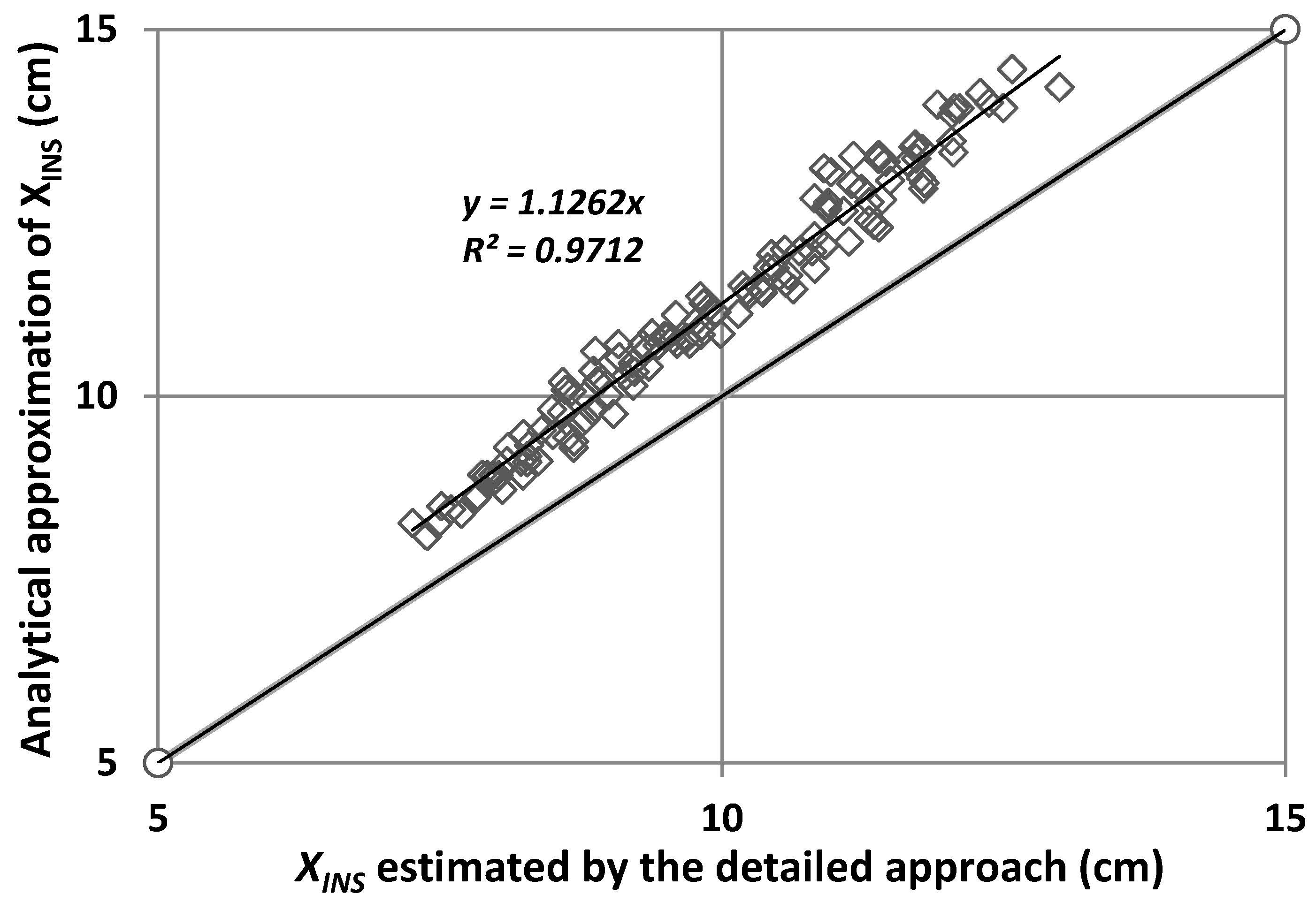
The optimum insulation thickness depends on the base temperature of the heated space, which in turn decreases by the addition of insulation. This induced variation should be taken into consideration when estimating optimum insulation thickness, otherwise errors up to 20% may arise. The analytical approach proposed here, although implicit, is easily solvable e.g., via a successive substitution or in a graphic, to rapidly lead to a more accurate estimation of the optimum insulation thicknesses rather than the previously suggested analytical relations.

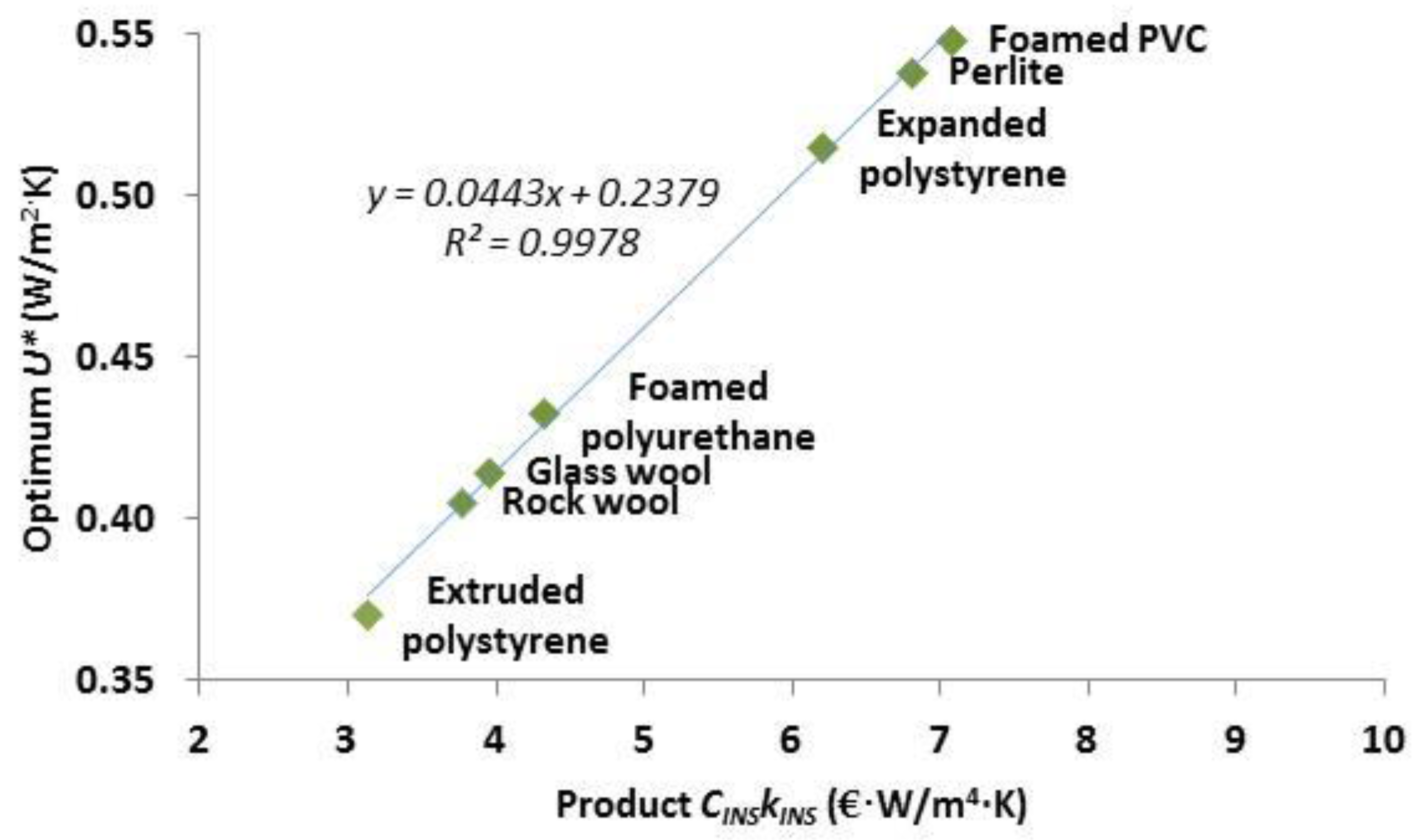
When selecting among alternative insulation materials, the most cost-effective is the one with the lower product when multiplying its cost by its thermal conductivity, C_INS·k_INS.

References

1. Balaras, C.; Gaglia, A.; Georgopoulou, E.; Mirasgedis, S.; Sarafidis, Y.; Lalas, D. European residential buildings and empirical assessment of the Hellenic building stock, energy consumption, emissions and potential energy savings. Build. Environ. 2007, 42, 1298–1314. [Google Scholar] [CrossRef]
2. Nikolaidis, Y.; Pilavachi, P.; Chletsis, A. Economic evaluation of energy saving measures in a common type of Greek building. Appl. Energy 2009, 86, 2550–2559. [Google Scholar] [CrossRef]
3. Gelegenis, J.; Diakoulaki, D.; Mavrotas, G.; Axaopoulos, P.; Samarakou, M.; Lampropoulou, H.; Giannakidis, G.; Giantzoudis, G. Holistic energy upgrade of dwellings. A resource management optimization approach. Int. J. Renew. Energy Res. 2015, 5, 998–1006. [Google Scholar]
4. Droutsa, K.; Kontoyiannidis, S.; Dascalaki, E.; Balaras, C. Mapping the energy performance of Hellenic residential buildings from EPC (energy performance certificate) data. Energy 2016, 98, 284–295. [Google Scholar] [CrossRef]
5. Hamelin, M.; Zmeureanu, R. Optimum Envelope of a Single-Family House Based on Life Cycle Analysis. Buildings 2014, 4, 95–112. [Google Scholar] [CrossRef]
6. Kaynakli, O. A review of the economical and optimum thermal insulation thickness for building applications. Renew. Sust. Energy Rev. 2012, 16, 415–425. [Google Scholar] [CrossRef]
7. Hasan, A. Optimizing insulation thickness for buildings using life cycle cost. Appl. Energy 1999, 63, 115–124. [Google Scholar] [CrossRef]
8. Comaklı, K.; Yuksel, B. Optimum insulation thickness of external walls for energy saving. Appl. Therm. Eng. 2003, 23, 473–479. [Google Scholar] [CrossRef]
9. Dombaycı, A.; Golcu, M.; Pancar, Y. Optimization of insulation thickness for external walls using different energy-sources. Appl. Energy 2006, 83, 921–928. [Google Scholar] [CrossRef]
10. Sisman, N.; Kahya, E.; Aras, N.; Aras, H. Determination of optimum insulation thicknesses of the external walls and roof (ceiling) for Turkey’s different degree-day regions. Energy Policy 2007, 35, 5151–5155. [Google Scholar] [CrossRef]
11. Kayfeci, M.; Keçebas, A.; Gedik, E. Determination of optimum insulation thickness of external walls with two different methods in cooling applications. Appl. Therm. Eng. 2013, 50, 217–224. [Google Scholar] [CrossRef]
12. Bolatturk, A. Optimum insulation thicknesses for building walls with respect to cooling and heating degree-hours in the warmest zone of Turkey. Build. Environ. 2008, 43, 1055–1064. [Google Scholar] [CrossRef]
13. Kurekci, N. Determination of optimum insulation thickness for building walls by using heating and cooling degree-day values of all Turkey’s provincial centers. Energy Buildings 2016, 118, 197–213. [Google Scholar] [CrossRef]
14. Yu, J.; Yang, C.; Tian, L.; Liao, D. A study on optimum insulation thicknesses of external walls in hot summer and cold winter zone of China. Appl. Energy 2009, 86, 2520–2529. [Google Scholar] [CrossRef]
15. Daouas, N. A study on optimum insulation thickness in walls and energy savings in Tunisian buildings based on analytical calculation of cooling and heating transmission loads. Appl. Energy 2011, 88, 156–164. [Google Scholar] [CrossRef]
16. Wati, E.; Meukam, P.; Nematchoua, M.K. Influence of external shading on optimum insulation thickness of building walls in a tropical region. Appl. Therm. Eng. 2015, 90, 754–762. [Google Scholar] [CrossRef]
17. Ozel, M. Effect of wall orientation on the optimum insulation thickness by using a dynamic method. Appl. Energy 2011, 88, 2429–2435. [Google Scholar] [CrossRef]
18. Yuan, J.; Farnham, C.; Emura, K.; Alam, M.A. Proposal for optimum combination of reflectivity and insulation thickness of building external walls for annual thermal load in Japan. Build. Environ. 2016, 103, 228–237. [Google Scholar] [CrossRef]
19. Özkan, D.; Onan, C. Optimization of insulation thickness for different glazing areas in buildings for various climatic regions in Turkey. Appl. Energy 2011, 88, 1331–1342. [Google Scholar] [CrossRef]
20. Kaynakli, O. Parametric Investigation of Optimum Thermal Insulation Thickness for External Walls. Energies 2011, 4, 913–927. [Google Scholar] [CrossRef]
21. Gelegenis, J. Diagrams for the correction of heating degree-days to any base temperature. Int. J. Green Energy 2010, 7, 376–386. [Google Scholar] [CrossRef]
22. Chartered Institution of Building Services Engineers (CIBSE). Degree-Days: Theory and Applications; TM41. CIBSE Report; CIBSE: London, UK, 2006. [Google Scholar]
23. Wikipedia. Normal Distribution. Available online: https://en.wikipedia.org/wiki/Normal_distribution (accessed on 10 February 2017).
24. Anderson, M.; Whitcomb, P. DOE Simplified: Practical Tools for Effective Experimentation, 2nd ed.; Productivity Press: New York, NY, USA, 2007. [Google Scholar]
25. Kalua, A. Envelope Thermal Design Optimization for Urban Residential Buildings in Malawi. Buildings 2016, 6, 1–32. [Google Scholar] [CrossRef]
26. Zalejska-Jonsson, A.; Lind, H.; Hintze, S. Energy-Efficient Technologies and the Building’s Saleable Floor Area: Bust or Boost for Highly-Efficient Green Construction? Buildings 2013, 3, 570–587. [Google Scholar] [CrossRef]
27. Ozel, M. Cost analysis for optimum thicknesses and environmental impacts of different insulation materials. Energy Build. 2012, 49, 552–559. [Google Scholar] [CrossRef]
28. Van Dijk, H.; Arkesteijn, C. Windows and Space Heating Requirements; Parametric Studies Leading to Simplified Calculation Method; The Netherlands National Report on Activities Within Step 5; TNO Inst. of Applied Physics: Delft, The Netherlands, 1987. [Google Scholar]
29. Yohanis, Y.; Norton, B. Utilization factor for building solar-heat gain for use in a simplified energy model. Appl. Energy 1999, 63, 227–239. [Google Scholar] [CrossRef]
30. Gelegenis, J. A simplified quadratic expression for the approximate estimation of heating degree-days to any base temperature. Appl. Energy 2009, 86, 1986–1994. [Google Scholar] [CrossRef]
31. Kapsalaki, M.; Leal, V.; Santamouris, M. A methodology for economic efficient design of Net Zero Energy Buildings. Energy Build. 2012, 55, 765–778. [Google Scholar] [CrossRef]
32. Axaopoulos, I.; Axaopoulos, P.; Panayiotou, G.; Kalogirou, S.; Gelegenis, J. Optimal economic thickness of various insulation materials for different orientations of external walls considering the wind characteristics. Energy 2015, 90, 939–952. [Google Scholar] [CrossRef]
33. Vincelas, F.F.C.; Tchuen Ghislain, T. The determination of the most economical combination between external wall and the optimum insulation material in Cameroonian’s buildings. J. Build. Eng. 2017, 9, 155–163. [Google Scholar] [CrossRef]
Figure 1. Correlation of consumption to the mean monthly ambient temperature, to demonstrate the effect of insulation and heat gains on the balance temperature.
Buildings 07 00015 g001
Figure 2. External insulation cost in retrofits, as a function of thickness.
Buildings 07 00015 g002
Figure 3. Variation of insulation costs, energy cost savings and accumulated net benefits with insulation thickness.
Buildings 07 00015 g003
Figure 4. Effect of cooling degree-days to optimum insulation thickness (use of XPS insulating material and as a fuel the natural gas, data from [12]).
Buildings 07 00015 g004
Figure 5. Gains utilization factor for various time constants, and estimations according to Equation (21) with kG = 1.2).
Buildings 07 00015 g005
Figure 6. Indicative flow-sheet of the proposed approach.
Buildings 07 00015 g006
Figure 7. Sketch of the heated space.
Buildings 07 00015 g007
Figure 8. Graphical solution of Equation (53), for the example.
Buildings 07 00015 g008
Figure 9. Optimum insulation thicknesses for the various orientations, according to the data of the example, and respective base temperatures before and after the insulation.
Buildings 07 00015 g009
Figure 10. Revealing the most significant parameters affecting optimum thermal transmittance.
Buildings 07 00015 g010
Figure 11. Variation of natural gas prices in Greece, during last three years.
Buildings 07 00015 g011
Figure 12. Optimum thermal transmittance values estimated in the sensitivity analysis, as compared to the respective values by applying the analytical expression.
Buildings 07 00015 g012
Figure 13. Correlation between the product CINS·kINS and the resulted optimum thermal transmittance U* for the alternative insulation materials.
Buildings 07 00015 g013