
Comparison of Space Heating Energy Consumption of Residential Buildings Based on Traditional and Model-Based Techniques


Faculty of Technology, University College of Southeast Norway, P.O. Box 203, N-3901 Porsgrunn, Norway
*
Author to whom correspondence should be addressed.
Buildings 2017, 7(2), 27; https://doi.org/10.3390/buildings7020027
Submission received: 18 December 2016
/
Revised: 6 March 2017
/
Accepted: 20 March 2017
/
Published: 23 March 2017
Abstract
:This paper presents a comparison of different scenarios in controlling the space heating systems in residential buildings. The space heating energy consumption of a three-storey residential building is estimated using traditional control methods (fixed-temperature schedule and fixed-time schedule) and a mathematical model-based control strategy. The model-based control technique takes the usage pattern of the building into account and operates the heaters based on the calculated heating time of the building. The results from the experiments confirm that the use of a model in heating control is the best option, which can save up to 1400 kWh and 320 kWh per year compared to a fixed-temperature schedule and fixed-time schedule, respectively.

1. Introduction
World energy use is rapidly growing and there are raised concerns over supply difficulties, depletion of energy resources, and heavy environmental impacts [1]. Simultaneously, the global contribution from buildings towards energy consumption has regularly increased the figures by between 20% and 40% in developed countries [1]. The building sector in the Europe accounted for nearly 41% of the total energy consumption in 2010 [2]. Residential buildings currently utilize 30% of the world average energy consumption and 25% of the average European Union energy consumption [3]. The energy use of these residential buildings is highly dependent on climate conditions, physical characteristics, appliances, occupant behaviors, and ownership [3]. Until recent years, the energy efficiency of buildings has been a relatively low priority. However, with the increase and awareness of energy use concerns and the advances in cost-effective technologies, energy efficiency is becoming a major concern to building owners both in commercial and residential sectors.
In this study, the focus is on saving space heating energy from heated residential buildings in cold climatic conditions, such as northern European countries. For instance, Scandinavian countries such as Norway usually remain under cold climate conditions during one-third of the year, and that results in high space heating energy use. To ensure the thermal comfort of the occupants and to avoid the freezing of water sources, it is important to heat the buildings. Further, it is necessary to heat up the building to a certain temperature even when the building is not occupied to ensure that water sources are not affected.
There are different control techniques used in buildings to control heating systems. They can be either classical controllers such as on-off and PID (Proportional-Integral-Derivative) or more advanced type controllers integrated with a mathematical model of the building [4]. Classical controllers have a simple structure and low initial cost, which makes them the most used controllers in HVAC (Heating, Ventilation and Air-Conditioning) systems in both commercial and residential buildings [5]. On-off control is one of the oldest techniques that is practiced in buildings for the purpose of energy saving and occupant thermal comfort. This simple, fast, and inexpensive feedback controller accepts only binary inputs. It is still being using in domestic and commercial buildings as the well-known thermostat [5]. While the thermostat is simple and inexpensive, it is often incapable of tracking the set point accurately and hence could be inefficient. Further, it is not versatile and effective in the long run [6,7,8].
The same as on-off control, PID control is also a feedback mechanism, which does not use knowledge/model of the interested system. It determines a deviation and adjusts the control signal according to that value. There are three separate control techniques used in a PID control algorithm: (i) proportional; (ii) integral; and (iii) derivative. The control signal is delivered based on a weighted sum of these three actions. Thermal process dynamics in a building is usually a slow responding process. Therefore, proportional control can be used in building temperature control with good stability and a reasonable offset [5]. The derivative term combats sudden load changes. Still, small amounts of measurement and process noise can cause large variations in the output due to the derivative term [5]. Even though PID control is easy to implement and has number of advantages [5], it may not be the most suitable controller for building control due to several reasons [9]. It requires three parameters to be tuned for each building zone, which is a time consuming task, and re-tuning may be inconvenient. PID controllers are unable to handle random disturbances, and therefore large deviations from the set point can occur. PID controllers may also have an overshoot of the adjusting parameter that can be a challenge when adjusting the temperature in a building. A standard PID controller assumes a single-input single-output system, which may cause unacceptable deviations in building systems, which are having a multi-variable behavior [9], since they operate at low energy efficiencies that may not be suitable in the long run [9].
The heat dynamics of a building have multi-variable behavior owing to the thermal interactions amongst different zones and the Heating, Ventilation, and Air-Conditioning (HVAC) system. Classical controllers in such a multi-variable building system may not deliver as high efficiencies as expected. Advanced controllers with a mathematical building heating model have the potential to address these constraints [9]. These algorithms are strictly designed for a particular building. Therefore, advanced controllers with a mathematical building heating model have the likelihood of saving more heating energy from buildings, while providing better occupant thermal comfort.
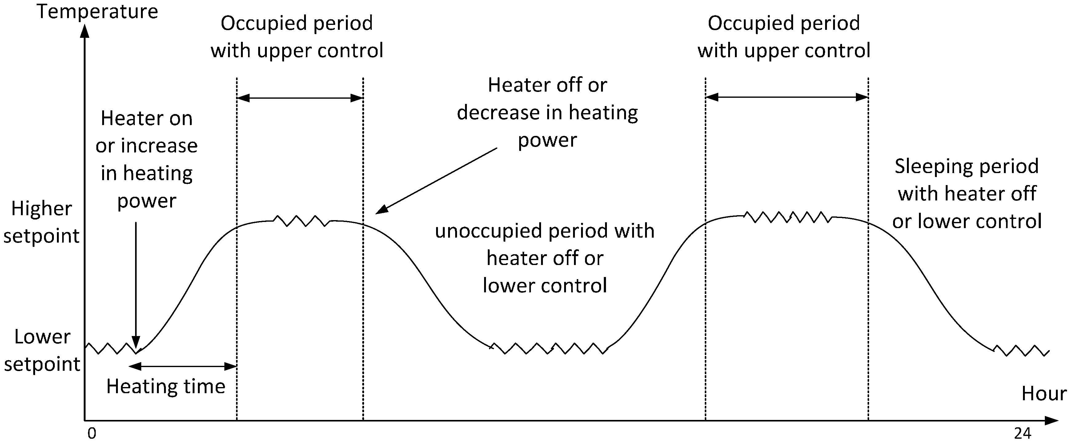
Non-residential buildings like schools and offices are intermittently occupied and have regular occupancy hours that make them easy to control for heating. Further, residential buildings can also be admitted as intermittently occupied spaces. These buildings can also be adjusted to have lower temperature set points during unoccupied periods and during nights. Comfortable temperatures need to be maintained only during the occupied times. Figure 1 illustrates the temperature variation of a typical residential building during a weekday. When the occupants are away or asleep, the temperature can be reduced to a value that will not affect the water sources inside the building. Before the occupants’ arrival or wakeup, the heating system must be switched on or the set point temperature must be increased such that the comfortable temperature is reached at the right time. If the temperature is in the comfort range before occupancy, energy is wasted, and, conversely, if the temperature reaches the comfort range after occupancy, it may be uncomfortable to the residents. Therefore, it is necessary to have an ‘optimal heating time’. The estimation of the heating time for small-scale buildings using physics-based mathematical models is explained further in [10], depending on changing climate conditions and changing heating loads. The possible amount of energy savings from these buildings are determined by the temperature drop during the unoccupied periods and nights, along with the temperature recovery period of the heating system.
The objective of this study is to demonstrate how much space heating energy can be saved by using a dynamic model of the building (with the estimation of heating time) for control. As mentioned earlier, advanced control techniques are integrated with a mathematical model of the interested system. When it comes to the control of buildings based on mathematical models, Model Predictive Control (MPC) has become one of the main interests. In the literature, examples on model based energy savings can mainly be found in the direction of MPC techniques. Some examples showing the energy saving potential of MPC and traditional controllers will be presented here for comparison purposes. However, this study has no focus on MPC and instead presents a general overview of the space heating energy saving potential of buildings when mathematical models are incorporated.
Morosan et al. have conducted a case study and presented that centralized and distributed Model Predictive Control (MPC) strategies can reduce the energy consumption by 13.4% compared to conventional P (Proportional), PI (Proportional-Integral), and On-Off control strategies for a selected day based on the occupancy [11]. In [12], there is an evaluation of the energy saving potential of buildings using MPC, classic PI control, and PI control with a dead zone. A resistor-capacitor network model is developed for a university building of 1500 m2. The total yearly energy consumption per square meter of the heated/cooled area is estimated to be 87.16, 133.94, and 125.55 kWh/m2 for the three techniques, respectively.
In order to estimate the energy savings, it is first necessary to estimate the space heating energy consumption of a building. Different types of mathematical models have been used in the past to estimate the space heating/cooling energy use of buildings. Statistical approaches such as regression [13,14,15], Artificial Neural Networks [16], and Support Vector Machines [17] are found in the literature for energy predictions. A combined physical and statistical approach has been used in [18]. A physics-based approach for the prediction of the energy consumption of buildings is explained in [10], and this method will further be used in this study to estimate space heating energy consumption based on different heating approaches to compare the possible energy savings from each approach.
The rest of the paper is structured to present the test building, description of different approaches in building heating, mathematical model development, results and discussion of the analyses, and concluding remarks.
2. The Test Building
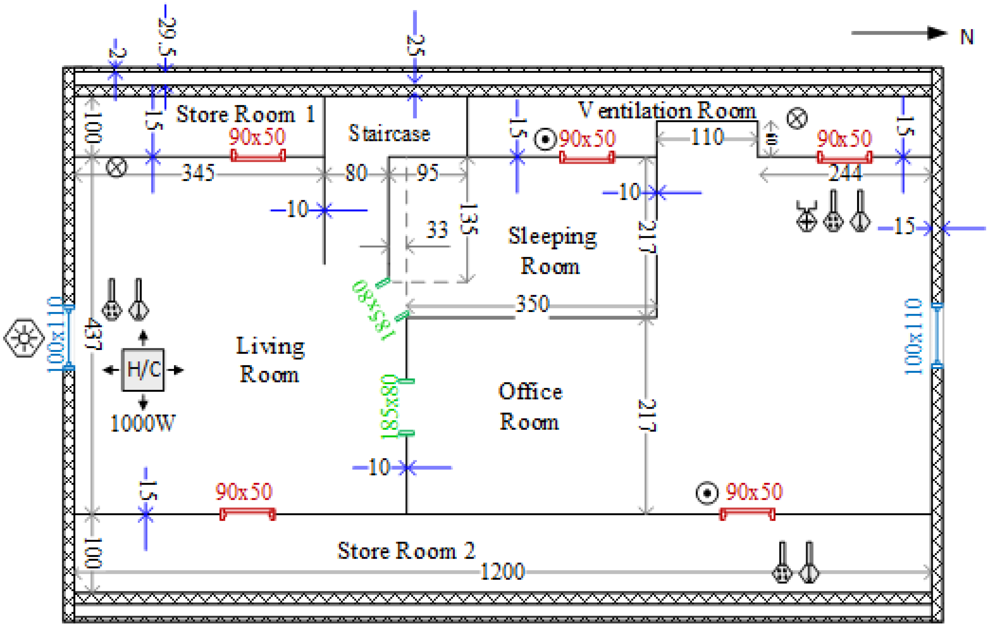
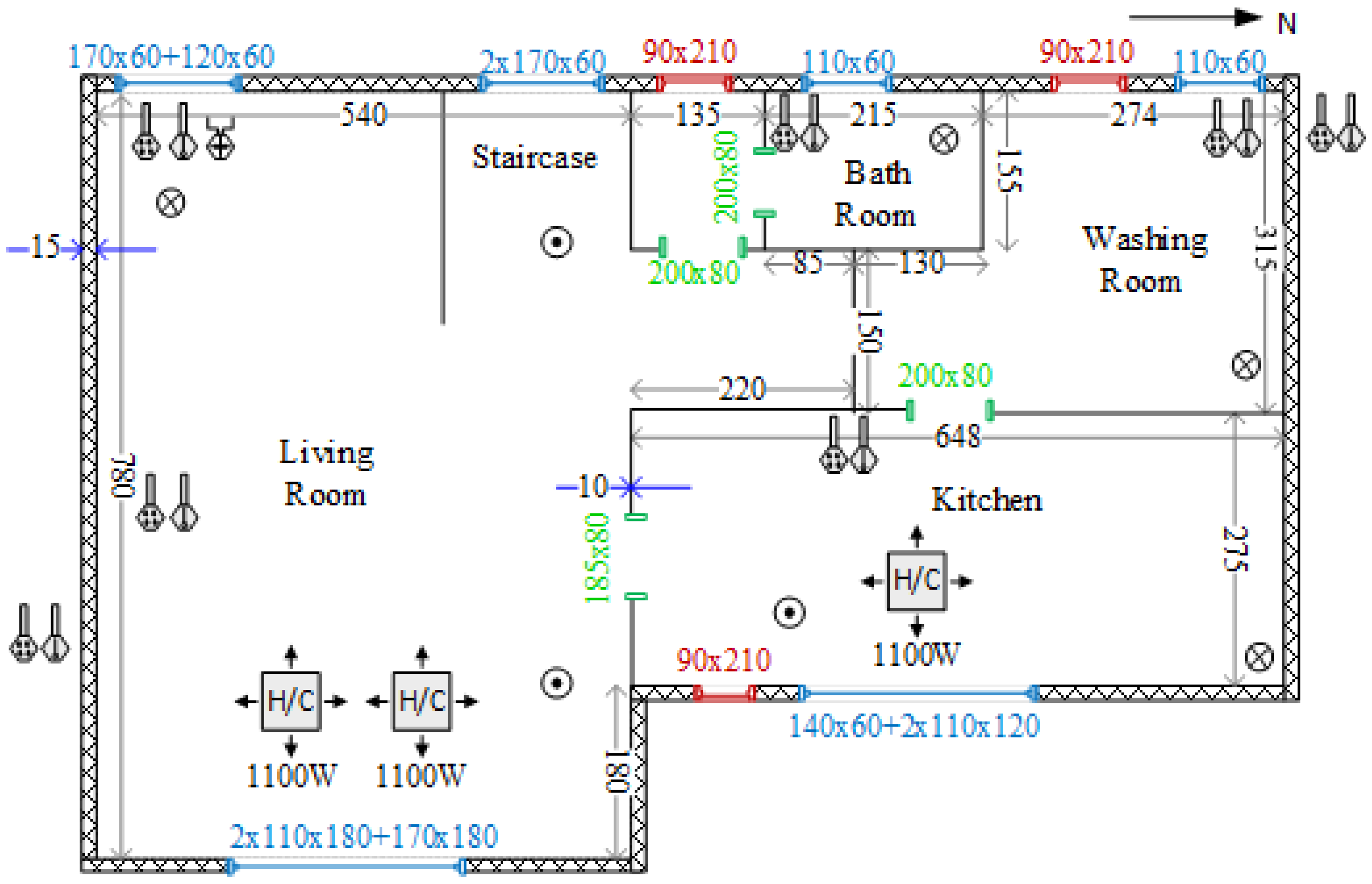
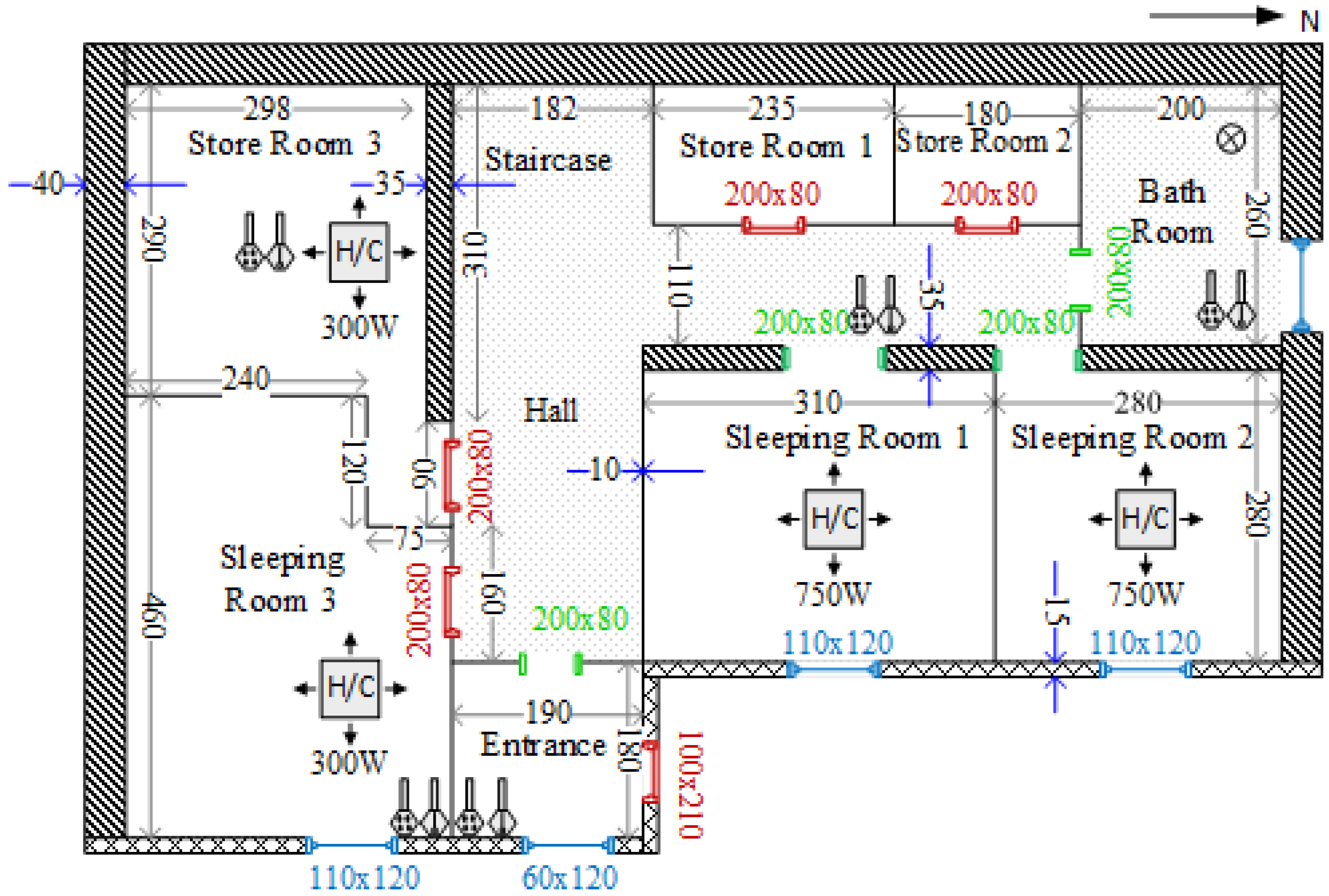
The building used for the study is a residential building built in 1987 and located in the southern part of Norway close to Langesund. The building consists of three stories: (i) attic; (ii) main floor; and (iii) basement. It has a balanced ventilation system installed in both the attic and the main floor with an integrated heat recovery system with 77% efficiency. The cumulative average air inflow rate into the building is 0.027 m3/s. The building is primarily constructed using wood and most of the walls and the floor of the basement are formed using concrete. The dimensions of the building with the dimensions of the windows and doors are illustrated in Figure 2, Figure 3 and Figure 4. The heights of the main floor and the basement are 240 cm and 235 cm, respectively. The attic has a triangular cross section and its highest height is 198 cm, which declines to 0 cm at the sidewalls. The thicknesses of the roofs and floors are 30 cm each.
There are electrical heaters on each floor of the building. The total heat supply to the building via electrical heaters is 6.95 kWh. Out of that, there is a floor heater in the basement, which supplies 550 W all the time. In addition to that, there are four personal computers operating inside the attic, which considerably heat the area. The approximate heat supply from all electrical appliances is 630 W. Supplementary to the electrical heaters, a wood burning stove is used on the main floor to heat the building, especially during freezing conditions, which is not modelled in this work. The locations where the temperature, relative humidity and solar irradiation sensors are positioned are also shown in Figure 2, Figure 3 and Figure 4. These sensors have a sampling frequency of 1 h.
The current heating control system in the building is based on a set of wireless remote controlled mains sockets turning the electrical heaters on and off at a fixed time schedule. Standard electrical heaters with an electrical thermostat are used. An application is used for turning the wireless remote controlled mains sockets on and off at a fixed schedule, as:
- Weekdays: on from 4:00 to 8:00 and 12:00 to 21:00 with a set point of 17 °C.
- Weekends: on from 3:00 to 23:00 with a set point of 17 °C.
A low set point temperature is not specified for the non-occupancy and sleeping periods. Instead, the heaters are switched off.
3. Case Studies
The space heating energy consumption of the building is estimated using a mathematical model developed in a MATLAB environment under different scenarios and the estimated values are compared with each other. The analysis is primarily a theoretical investigation, and all the cases are summarized below. All case studies estimate the temperatures and energy consumptions based on the input measurements obtained for five week days from 24 to 28 November 2014. The input variables (outside temperature, outside relative humidity, inside relative humidity, and solar irradiation) used in the study are plotted in Figure 5 for the experimental period. The real inside temperature data for the mentioned period is also collected for calibrating the model parameters, and these parameters will be used in all other cases to assess the space heating energy consumption.
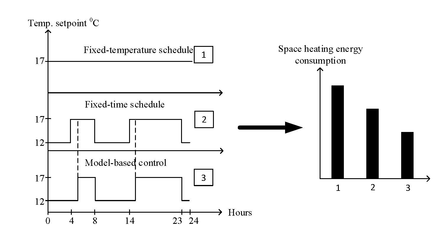
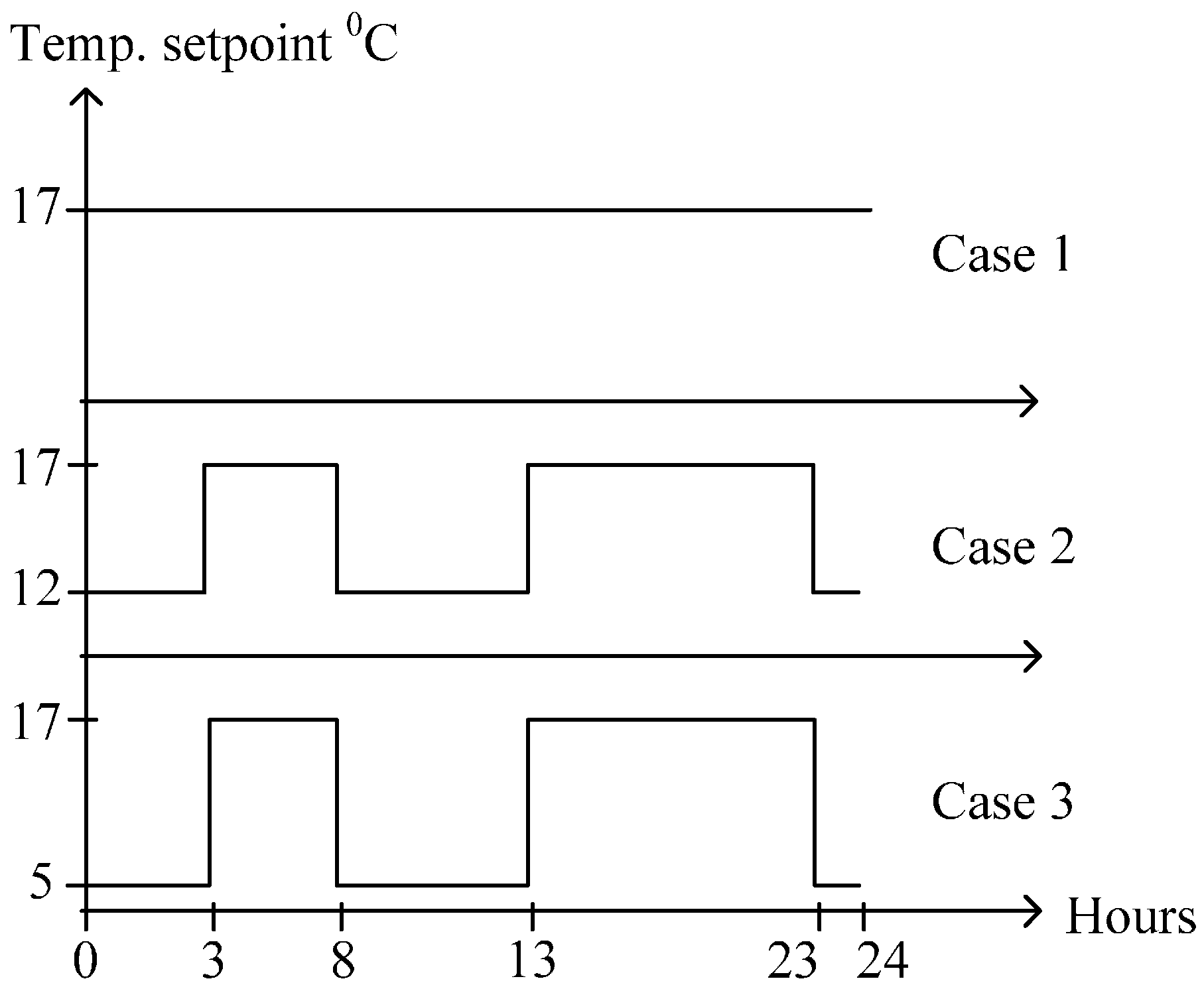
- Case 1: Estimation of space heating energy consumption for a constant inside temperature of 17 °C (comfort temperature) throughout the five days in the test building (fixed temperature schedule).
- Case 2: Estimation of space heating energy consumption according to time-based control such that the heaters switch between different temperature set points at pre-selected times of the day (fixed time schedule). The heating system is configured to maintain two temperature set points; comfort temperature (17 °C) and non-occupancy temperature (12 °C) for occupied and non-occupied (or sleeping) periods. A fixed period of three hours is selected as the heating time of the building before occupant arrival/wake up.
- Case 3: This case is similar to case 2, with the low temperature set point (non-occupancy and sleeping) equal 5 °C instead of 12 °C (fixed time schedule). A heating time of 3 h is assumed for case 3 as well.
- Case 4: Estimation of space heating energy consumption according to the usage pattern of the building with the help of heating time estimations via a mathematical model of the building. Instead of using a fixed heating time, now the real heating time is estimated using a dynamic model. Low and high temperature set points (comfort temperature of 17 °C and non-occupancy/sleeping temperature of 12 °C) are used here as well.
- Case 5: This is an extension of Case 4, and it estimates the space heating energy consumption if the occupants are one day away from the building. This represents a day off at work or a short holiday during which the occupants are one day away from the building and addresses possible energy savings when a model is used in heating system control.
- Case 6: This is an extension of Case 4, and it estimates the space heating energy consumption if the occupants are two days away from the building, such as going away on the weekend. This case is a good example to observe how much energy can be saved when the occupants are away from the building for a long period.
Figure 6 illustrates the variation of temperature set points with respect to time for Cases 1, 2, and 3 during a one-day period.
4. The Modelling Approach
The mathematical model of the building is the basis for advanced controller implementation. The mathematical model used in estimating the temperature variation, heating time, and the space heating energy consumption is a continuous time dynamic model developed for a single-zone building. The building unit is considered a control volume. The model is expressed in terms of state-space variables, and a lumped parameter approach has been used. A detailed description of the model development can be found in [19]. Equations (1)–(10) represent the model, and Table 1 describes all the symbols.
The mass and energy balances formulate the heating model for the specified test building. Mass and energy balance equations for the air inside the building unit are given by Equations (1) and (2). Ventilation plays a leading role in the convective mode of heat transfer in buildings. The application of mass balance to the airflow is, therefore, vital in the modeling of ventilated spaces. The building has a balanced ventilation system installed in it. Both the attic and the main floor are supplied with ventilation by mechanical means and are integrated with a heat recovery system. When it comes to the modeling of ventilation, infiltration is neglected, as it is a small fraction compared to large-scale mechanical ventilation. When developing the energy balance equation, only the internal energy of the air is considered, while kinetic and potential energies are neglected.
The discretized transient heat equation is used to model the walls, floor, and roof of the building unit, represented by Equations (3)–(5). These components are made out of several layers of dissimilar materials such as wood, concrete, and insulation. However, layers are lumped into one element of the uniform thermal properties for simplicity and hence j = 1. Therefore, Tsj+1 and Tsj represent outside and inside surface temperatures of each component. The thermal mass of the household furniture is represented as a spherical object and modeled using the heat equation in spherical coordinates after discretization using the finite difference method (Equation (6)). When modeling the furniture, one spherical layer is considered as same as other building components and therefore Tsj+1,fur and Tsj,fur represent outside surface temperature and center temperature of the sphere..
The total heat flow from other sources than ventilation () to the building unit is given by Equation (7), while Equation (8) estimates the heat loss through the building envelope. The test building is equipped with heat recovery ventilation to heat the incoming cold air. The incoming air temperature through this system to the building unit is given by Equation (9). Equation (10) estimates the energy consumed by the heaters to raise the temperature of the building unit.
5. Results and Discussion
The aforementioned mathematical model is implemented in MATLAB for the test building and solved using ode15s solver. The model consists of six state variables, including indoor density, indoor temperature, and temperatures of the building components. Under the results, the space heating energy consumption of the test building from 24 to 28 November 2014 is first presented. Next, space heating energy consumptions estimated for each case study will be given with the relevant temperature variation graph.
Usually the comfortable temperature range inside a building falls between 20 °C and 22 °C. However, in the following cases, the comfortable temperature set point of the building is taken as 17 °C to be compatible with the real inside temperature variation of the building during the test period.
The floor heater in the basement (550W) is continuously operating, and it is taken into consideration only for estimating the energy consumption during 24 to 28 November 2014. However, for the rest of the cases, this floor heater is assumed to operate intermittently, the same as other heaters.
5.1. Model Calibration and Error Analysis
The model parameters need to be tuned to have a good match between the measurements and the simulated results. There are different approaches for the calibration of building heating models, and these are explained in [20]. The MATLAB model used in this study is calibrated manually by varying the most uncertain parameters, such as the overall heat transfer coefficients and thermal diffusivities, in order to have a good match between the predicted and measured inside temperature profiles during the period 24 to 28 November 2014. The Norwegian Building Technical Regulations (TEK10) present the upper/lower limits for these parameters relevant to Norwegian buildings, which helped in assigning the parameter values. However, there are challenges in calibrating the physical parameters with respect to experimental data that may result in bad physical interpretation of the parameters. More advanced techniques such as Kalman filtering can be integrated into the model to get a good approximation of the parameters [21], which is not the focus of this work. The parameters associated with the air, building enclosure, and furniture used in the simulation are presented in Table 2. The given parameters and input variables (Figure 5) are independent of the case number.
The predicted temperature variation inside the test building for the experimental period based on the calibrated parameters and the measurements is presented in Figure 7, which includes the heater activity graph. The model considers the whole test building with three floors as a single unit and represents the average situation inside the building. In the simulation, the air temperature is controlled using an on-off controller to maintain the temperature set points, which is also the reason for frequent fluctuations in the predicted temperature profile.
The predictions are slightly diverged from the real measurements on some days. The error is due to dealing with any parameters and model approximations that may affect the output of the model. Even though the set point temperature is 17 °C from 4:00 to 8:00, the calculated average building temperature is about 16 °C during this period. The three floors of the building have different heating strategies, and a set of distributed measurements are used for estimating a mean value for the temperature and humidity of each floor. Usually the basement has the lowest temperature, which has affected the average temperature of the whole building during this period. The use of average temperature may also cause deviations in model calibration. Model calibration error can be reduced by individually modelling each floor of the building instead of assuming them to be one unit [22]. Further, the temperature measurements from the first day could have been affected by the activities of the previous day, of which the model was unaware, and have caused deviations. The other deviations in the predictions could be due to the undetected behaviors of the occupants such as use of the wood oven, short openings of any windows and/or doors, or changing the heater setups, to mention a few possibilities. In addition, the predictions from the model seem to have fast dynamics compared to the real measurements. This could happen when the modelled thermal inertia is lower than the actual thermal inertia. The estimated actual space heating energy consumption is 249.4 kWh, which could be slightly different in reality owing to the above-mentioned modelling deficiencies.
5.2. Case Studies
Figure 8 illustrates the inside temperature variation for Cases 1, 2, 3, and 4, respectively. In Case 1, a constant inside temperature of 17 °C is maintained throughout the five days. It is important to maintain a comfortable temperature for the occupants if a fixed-temperature schedule is of interest. This will increase the space heating energy consumption as heaters are operating even during the unoccupied periods. The temperature fluctuations in Case 1 is owing to the action of the simulated on-off controller with an operation bandwidth of ±0.25 °C. The estimated space heating energy consumption is 291.9 kWh for this scenario.
Case 2 is an example of a time-based control system, which is comparable to the current control system installed. Two temperature set points are selected such that one is a comfortable temperature (17 °C) and the other is a lower temperature (12 °C) with a 5 °C difference. The heaters are configured to switch between these set points at pre-selected times of the day. In this experiment, the controller switches to 17 °C at 3:00 and 13:00 and to 12 °C at 8:00 and 23:00. The controller switches to a higher temperature set point three hours before occupancy or wake up. The estimated space heating energy consumption is 261.4 kWh.
Instead of switching to a lower set point of 12 °C, in Case 3, the heaters switch to 5 °C. The water sources can freeze if the inside temperature goes below 5 °C. Therefore, it is highly important to fix the lower set point at least at 5 °C instead of completely switching the heaters off. This is a good strategy to save energy when the outside temperatures are high enough to maintain the building temperature at non-freezing values. However, the results obtained for Case 2 and Case 3 are similar in this experiment because the outside temperature is high enough and it does not go below 0 °C during the considered period. Further, the thermal mass of the building may have a high value, which also maintains the inside temperature above the 12 °C limit during unoccupied periods. Therefore, in both Case 2 and Case 3, the heaters are not operating from 8:00 to 13:00 and 23:00 to 3:00. Still, the effect of the outside temperature can be observed from the inside temperature graphs of Cases 2 and 3 as they reach the lowest inside temperature just after 3.5 days. The same variation can be seen in the outside temperature profile presented in Figure 5.
Both Case 2 and Case 3 are based on the assumption that the three hours pre-heating time is sufficiently long enough to raise the indoor temperature to a comfortable temperature, starting from a lower value. It was selected as a starting point when the control is not model-based, and it was postulated that it would cover 80% of the weather conditions while not causing too much energy wastage. This hypothesis was accurate for the test building under the specified weather conditions. However, on an extremely cold day, the pre-heating time could be longer than 3 h, and thermal comfort will not be achieved by the time of the occupants’ arrival. On the other hand, when the outside temperatures are noticeably high, the pre-heating time might be shorter than 3 h, causing unnecessary energy wastage. Both of them are disadvantages of having a traditional control method with a fixed pre-heating time. These deficiencies can be eliminated by using a model-based control associated with heating time estimation. In such systems, the model estimates the heating time based on inside conditions and outside weather conditions and initiates the heating at the right time to achieve thermal comfort and energy savings. Case 4 will provide an example of such a model-based system.
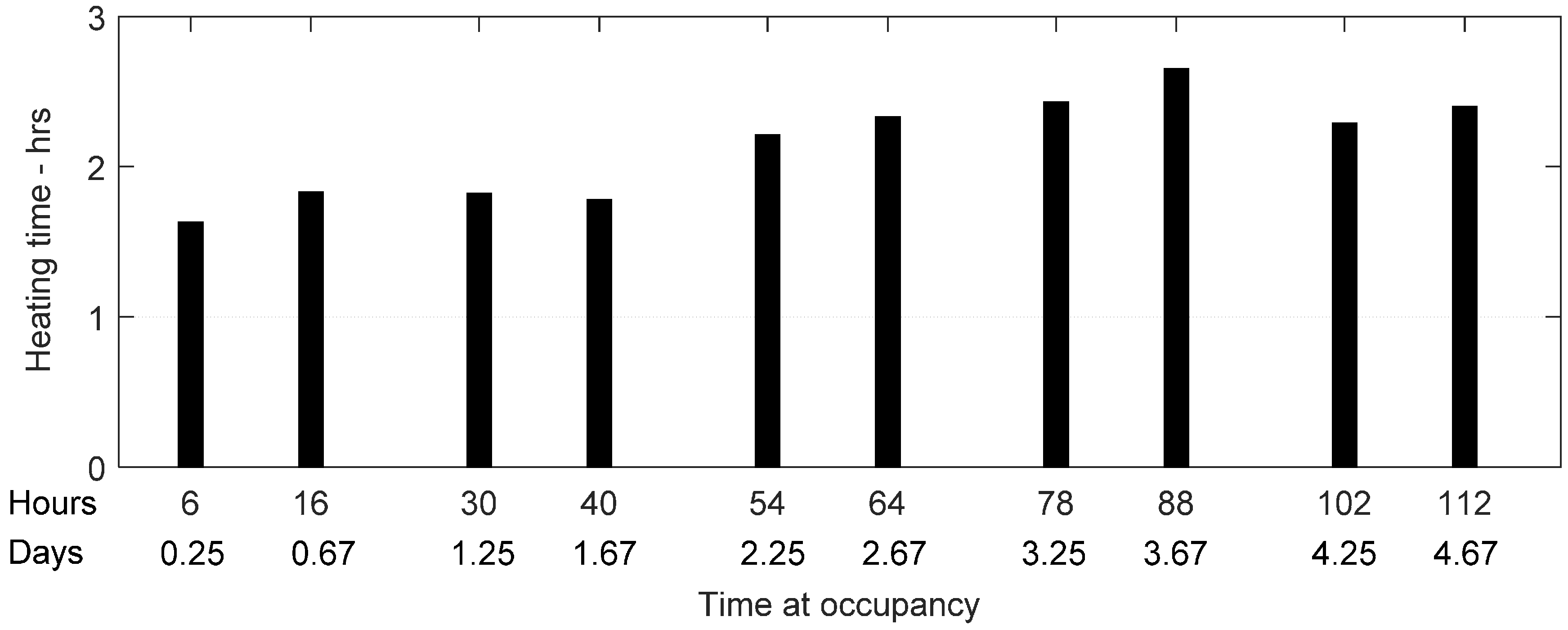
In Case 4, it is anticipated that occupants wake up at 6:00 and leave for work at 8:00. Further, they come back home at 16:00 and go to bed at 23:00. Therefore, the occupants use the building for 2 h in the morning and 7 h in the evening. The building must be heated to a comfortable temperature only during these 9 h, and during the rest of the time, the temperature set point can be reduced. Case 4 is different from Cases 2 and 3 owing to the heater operation based on the heating time of the building. The heaters switch to a high temperature set point before a specified time, which is equivalent to the estimated heating time based on the weather conditions. The estimated heating times by means of the mathematical model of the building are illustrated in Figure 9. The maximum heating time is 2.65 h, and minimum heating time is 1.63 h. When the heaters are operated based on these heating times, the estimated space heating energy consumption is 252.5 kWh.
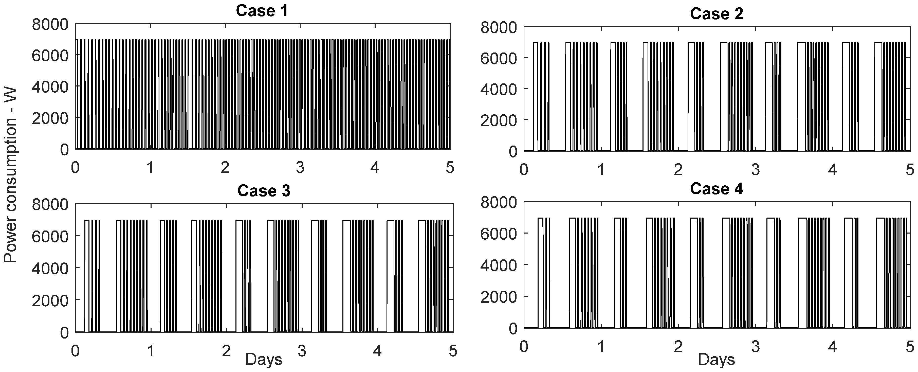
The power supply from the heating system at each time instant during the mentioned period for the first four cases is demonstrated in Figure 10. In Case 1, the heater activity is very intensive owing to the maintenance of the high temperature inside the building all the time. Case 2 and Case 3 have equivalent heater operation patterns that are not as rigorous as Case 1. When observed carefully, Case 4 has the least intensity compared to the other three cases. However, the pattern is quite analogous to those in Cases 2 and 3.
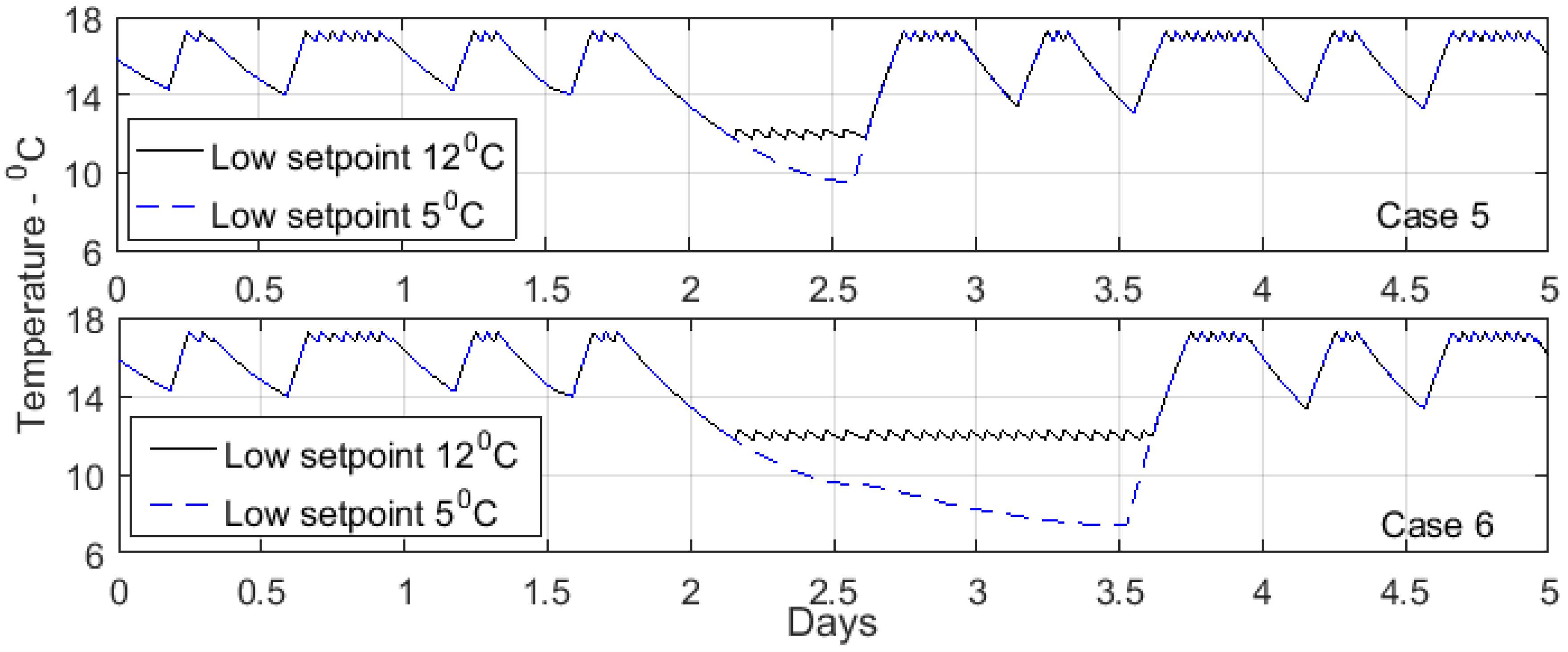
The temperature variations for Case 5 and case 6 are illustrated in Figure 11. In Case 5, it is assumed that the occupants are away from the building for 1.75 to 2.75 days (42 to 66 h). The estimated heating time before the occupants’ arrival is 3.2 h if the temperature is maintained at 12 °C during the unoccupied one-day period. It is necessary to bring the inside temperature to 17 °C at 66 h. Therefore, the heaters are switched to a high temperature set point at 62.8 h to achieve this outcome. During the rest of the time, the heater operation is similar to Case 4. The estimated space heating energy consumption is 234.5 kWh. If the temperature set point is 5 °C during this one-day period, the heating time is 4.25 h and the energy consumption is 229.3 kWh, which is a 5.2 kWh saving.
In Case 6, the occupants are away from the building for 1.75 to 3.75 days (42 to 90 h), i.e., two days, which could be a weekend. The heating times of the building at the occupants’ arrival is estimated as 3.24 and 5.4 h for maintaining the non-occupancy set point at 12 °C and 5 °C, respectively, during the two day period. The space heating energy consumptions for these two strategies are 208.5 and 178.1 kWh. With a lower set point of 5 °C, an extra 30.4 kWh can be saved.
These two cases represent the temperature in the building during holidays and weekends. When the occupants are away from the building for an extended time, it is a good opportunity to save energy by lowering the non-occupancy set point to a value that does not affect the inside water sources. If a traditional method, as presented in Cases 2 and 3, is used to control the heating, then the heaters have to be switched on 3 h before the occupants’ arrival. However, the estimated heating times for these two cases are above 3 h, and the consequence is occupant discomfort at the time of arrival. By using a model-based control method, this issue can be solved. Further, based on the results, it is worth being aware of the weather conditions before making decisions on heater operation. When the building is not in use, it is obligatory to maintain the building at a temperature above zero, between 5 and 10 °C. A controller integrated with a mathematical model and weather predictions can put the heaters to the required conditions after a disturbance evaluation.
The heater activity for Cases 5 and 6 is presented in Figure 12 during the five day experimental period. According to the figure, when the low temperature set point is 5 °C, the heating system is switched off, which helps to save energy.
5.3. Energy Predictions
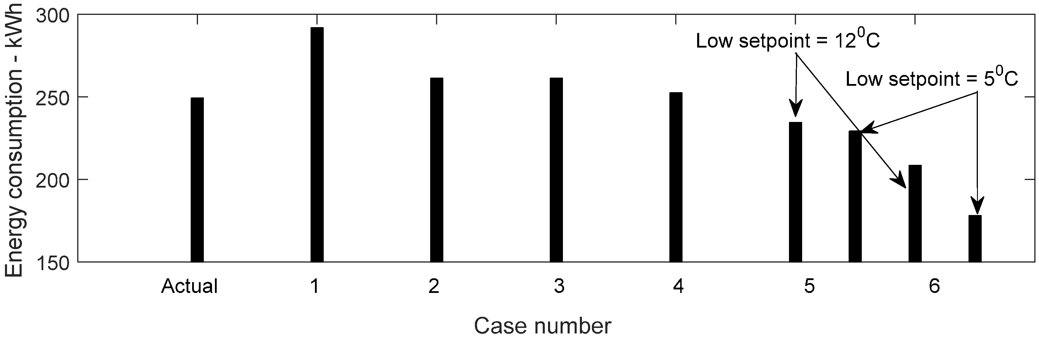
The derived mathematical model predicts the space heating energy consumption for the simulated five day period. A comparison of the space energy consumption for each case is presented in Figure 13 and Table 3. Even though the predicted actual energy consumption is given in the graph, it is not wise to compare it with the other cases as it has a different inside temperature variation pattern. It can be observed that maintaining a fixed comfortable temperature throughout the period results in the highest energy consumption (Case 1). Case 2 and Case 3 have equal results. The lowest energy consumption for five days of occupancy is observed in Case 4 out of the first four cases. Therefore, it is worth using a mathematical model to estimate the heating time according to the usage pattern of the building for control purposes. This kind of system can make wise control decisions based on the weather predictions before the system faces new instabilities.
The possible energy savings by setting the temperature set point down to 5 °C is trivial for short vacant periods like one day (Case 5). However, the savings are around 15% when this is applied for periods above one day (Case 6).
If the building heating system is controlled using a mathematical model based on the usage pattern and heating time (Case 4) instead of using a traditional control system as in Case 2, 8.9 kWh can be saved over five days, which is approximately 320 kWh of savings for the six cold months during a year. Most residential buildings use simple on-off controllers with a fixed temperature set point, like in Case 1, to operate heaters. If they transform the available system to model-based control, they can save up to 1400 kWh per year.
5.4. Improvements
One of the main limitations of model-based heating control is the discrepancy between the actual and simulated results, which can also be detected from Figure 7. Before using a specific model for control purposes, it is necessary to overcome this disadvantage for better performance of the system. The use of good model calibration techniques is the basis for achieving minimal discrepancy between the measured and simulated results. Kalman filtering and its extensions are heavily used today to get better estimations from models. Further, the model adaption (adaptive models with automatic calibration) to the real situation (real inside and outside conditions) is a good approach to minimize deviations.
Many measurement systems available today have a CO2 sensor included for measuring the quality of the inside air. These measurements can be used for extending the system with a usage pattern model as well. A simple model, based on the CO2 values, can be used to estimate when the building is in use and not in use to optimize the time schedule for switching to a high set point temperature.
The present study addresses the space heating energy saving potential using a control system integrated with a physics-based model. However, not only physics-based models but also data-driven or grey box models can be used for this purpose with any type of advanced control mechanism such as model predictive control, adaptive control, or optimal control strategies. Grey models might be a good solution in order to achieve a good model adaption to the real conditions (inside and outside) of the building.
6. Conclusions
This paper presents the application of a dynamic modelling approach for determining the space heating energy consumption of buildings. The focus was to figure out if the use of a mathematical model in space heating could save energy compared to the use of classical control methods. The suggested approach was tested on a three-storey residential building located in Norway, and several cases were defined to compare the energy consumptions. The results from the experiments confirm that use of a model to control the heating based on heating time estimations and usage patterns is the best option in terms of saving space heating energy and achieving thermal comfort. Maintaining a fixed-temperature schedule has the highest energy consumption of all. Having a time-based control system can save some amount of energy, while it is not the optimum.
Extending the current time based controller system for the electrical heaters with a mathematical model of the building will be a valuable improvement. This way, an optimum turn on time can be projected for the electrical heaters, saving more energy.
Any embedded systems running the on-off time control system like a BEMS (Building Energy Management System), as described in Case 2 and Case 3, can be extended at low cost to Case 4 to save more energy. The extension will be to include the building model into the software application running on the BEMS. An outside temperature sensor device must also be included in some BEMS; however, many BEMS already have this sensor device installed [4].
Acknowledgments
This study was funded by University College of Southeast Norway, Porsgrunn, Norway.
Author Contributions
Degurunnehalage Wathsala Upamali Perera developed the mathematical model, designed the experiments, performed the analysis, and was responsible for preparing the manuscript. Nils-Olav Skeie provided experimental data, designed the experiments, provided ideas to analyze the results, and revised the manuscript in all versions.
Conflicts of Interest
The authors declare no conflict of interest.
References
- Perez-Lombard, L.; Ortiz, J.; Pout, C. A review on buildings energy consumption information. Energy Build. 2008, 40, 394–398. [Google Scholar] [CrossRef]
- European Commission. Financial Support for Energy Efficiency in Buildings 2013; Tech rep; European Commission: Brussels, Belgium, 2013. [Google Scholar]
- Swan, L.G.; Ugursal, V.I. Modeling of end-use energy consumption in the residential sector: A review of modeling techniques. Renew. Sustain. Energy Rev. 2009, 13, 1819–1835. [Google Scholar] [CrossRef]
- Levermore, G.J. Building Energy Management Systems: Applications to Low-Energy HVAC and Natural Ventilation Control; Taylor & Francis: London, UK, 2000. [Google Scholar]
- Mirinejad, H.; Sadati, H.; Maryam, G.; Hamid, T. Control Techniques in Heating, Ventilating and Air Conditioning (HVAC) Systems 1. J. Comput. Sci. 2008, 4. [Google Scholar] [CrossRef]
- Peffer, T.; Pritoni, M.; Meier, A.; Aragon, C.; Perry, D. How people use thermostats in homes: A review. Build. Environ. 2011, 46, 2529–2541. [Google Scholar] [CrossRef]
- Wen, J.; Smith, T. Review of thermostat time constant on temperature control and energy consumption. In Sensors for Industry; IEEE: Rosemont, IL, USA, 2001. [Google Scholar]
- Maheshwari, G.P.; Al-Taqi, H.; Suri, R.K. Programmable thermostat for energy saving. Energy Build. 2001, 33, 667–672. [Google Scholar] [CrossRef]
- Virk, G.S.; Cheung, J.M.; Loveday, D.L. Development of adaptive control techniques for BEMs. In Proceedings of the International Conference on CONTROL ’91, Edinburgh, UK, 25–28 March 1991. [Google Scholar]
- Perera, D.; Skeie, N.-O. Estimation of the Heating Time of Small-Scale Buildings Using Dynamic Models. Buildings 2016, 6, 10. [Google Scholar] [CrossRef]
- Moroşan, P.-D.; Bourdais, R.; Dumur, D.; Buisson, J. Building temperature regulation using a distributed model predictive control. Energy Build. 2010, 42, 1445–1452. [Google Scholar] [CrossRef]
- Martincevic, A. Improvement of Building Energy Efficiency through Use of Advanced Control and Estimation Techniques. Available online: https://manualzz.com/doc/14083378/improvement-of-building-energy-efficiency-through-use-of-... (accessed on 22 November 2016).
- Westergren, K.-E.; Högberg, H.; Norlén, U. Monitoring energy consumption in single-family houses. Energy Build. 1999, 29, 247–257. [Google Scholar] [CrossRef]
- Lam, J.C.; Wan, K.K.W.; Liu, D.; Tsang, C.L. Multiple regression models for energy use in air-conditioned office buildings in different climates. Energy Convers. Manag. 2010, 51, 2692–2697. [Google Scholar] [CrossRef]
- Braun, M.R.; Altan, H.; Beck, S.B.M. Using regression analysis to predict the future energy consumption of a supermarket in the UK. Appl. Energy 2014, 130, 305–313. [Google Scholar] [CrossRef]
- Li, K.; Hu, C.; Liu, G.; Xue, W. Building’s electricity consumption prediction using optimized artificial neural networks and principal component analysis. Energy Build. 2015, 108, 106–113. [Google Scholar] [CrossRef]
- Jung, H.C.; Kim, J.S.; Heo, H. Prediction of building energy consumption using an improved real coded genetic algorithm based least squares support vector machine approach. Energy Build. 2015, 90, 76–84. [Google Scholar] [CrossRef]
- Lü, X.; Lu, T.; Kibert, C.J.; Viljanen, M. Modeling and forecasting energy consumption for heterogeneous buildings using a physical-statistical approach. Appl. Energy 2015, 144, 261–275. [Google Scholar] [CrossRef]
- Perera, D.W.U.; Pfeiffer, C.F.; Skeie, N.-O. Modelling the heat dynamics of a residential building unit: Application to Norwegian buildings. Model. Identif. Control 2014, 35, 43. [Google Scholar] [CrossRef]
- Djuric, N.; Novakovic, V.; Frydenlund, F. Heating system performance estimation using optimization tool and {BEMS} data. Energy Build. 2008, 40, 1367–1376. [Google Scholar] [CrossRef]
- Perera, D.W.U.; Perera, M.A.S.; Pfeiffer, C.F.; Skeie, N.-O. Structural observability analysis and EKF based parameter estimation of building heating models. Model. Identif. Control (MIC) 2016, 37, 171–180. [Google Scholar] [CrossRef]
- Perera, D.W.U. Mathematical Models for Real Time Estimation of Space Heating in Buildings; University College of Southeast Norway: Notodden, Norway, 2016. [Google Scholar]
Figure 1.
The temperature variation pattern of a residential building when the occupancy is known.

Figure 2.
Sketch of the attic of the test building (All measurements are in cm).

Figure 3.
Sketch of the main floor of the test building (All measurements are in cm).

Figure 4.
Sketch of the basement of the test building (All measurements are in cm).

Figure 5.
The variation of input variables from 24 to 28 November 2014.
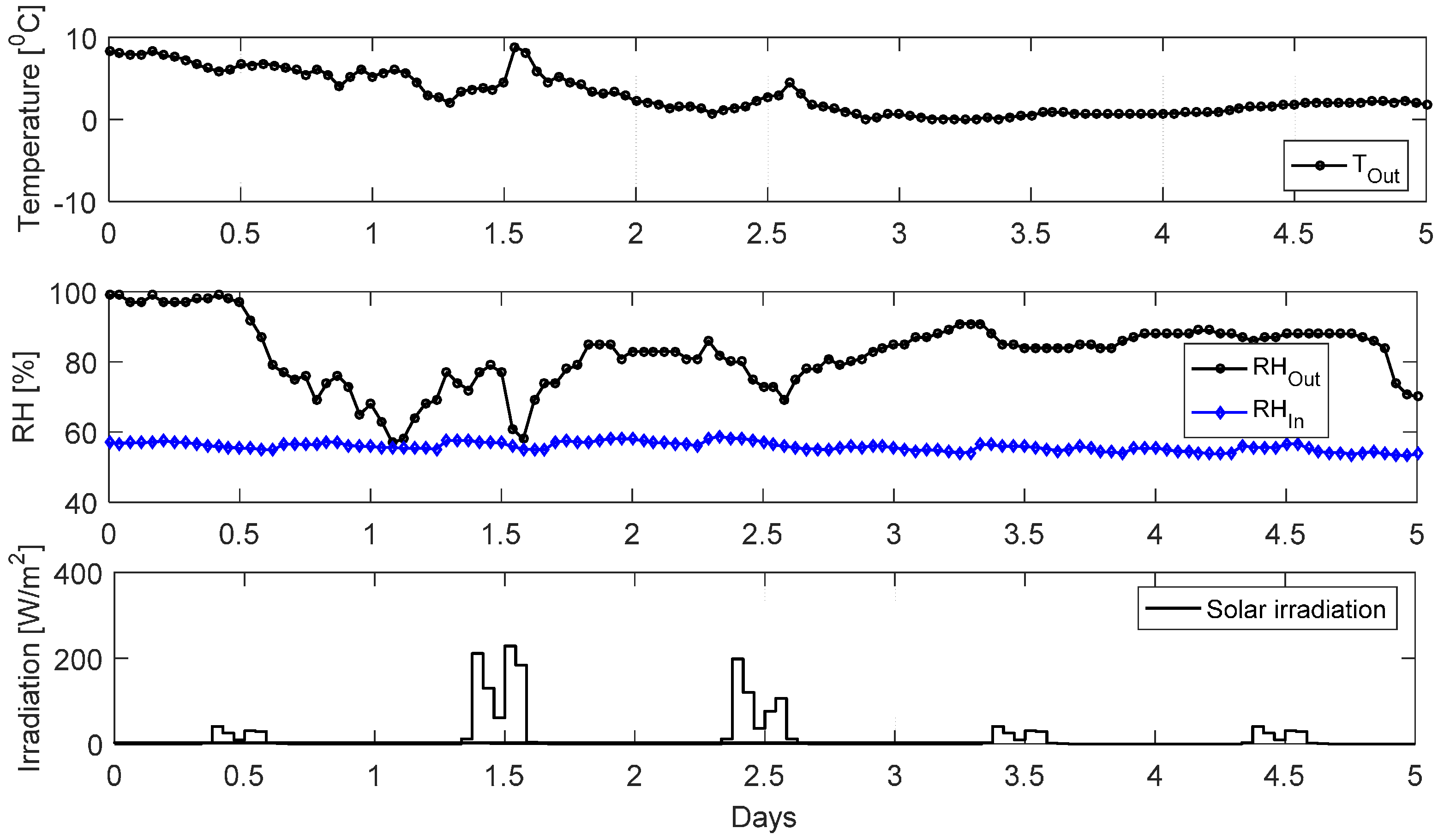
Figure 6.
Variation of temperature set points during a one-day period.

Figure 7.
Predicted and measured temperature variation inside the test building. The heater activity shown in the lower graph is based on the power consumption.
Figure 7.
Predicted and measured temperature variation inside the test building. The heater activity shown in the lower graph is based on the power consumption.
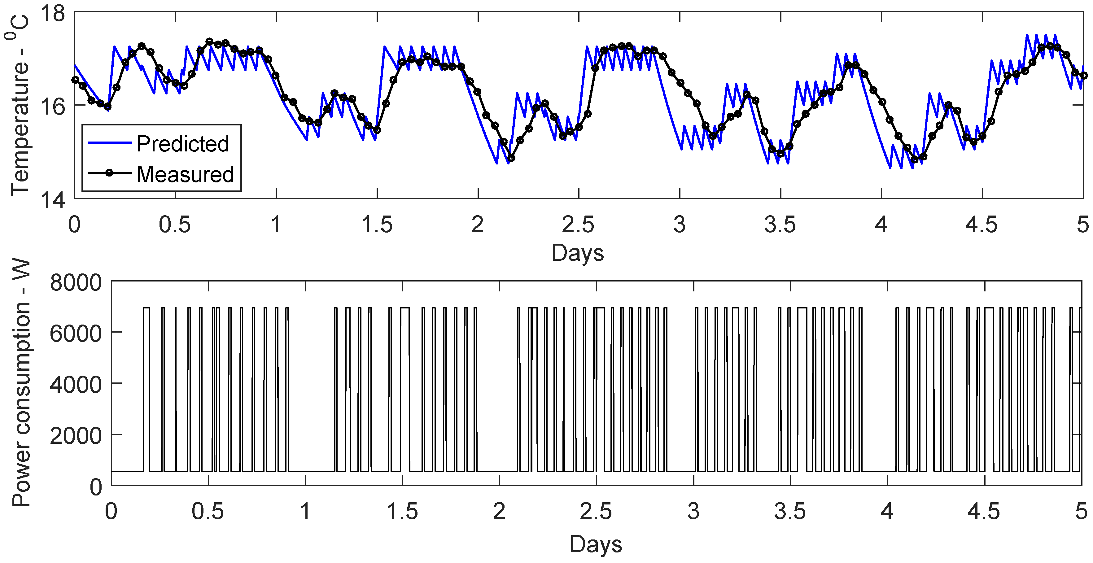
Figure 8.
Predicted temperature variation inside the test building for Case 1, Case 2, Case 3, Case 4.
Figure 8.
Predicted temperature variation inside the test building for Case 1, Case 2, Case 3, Case 4.
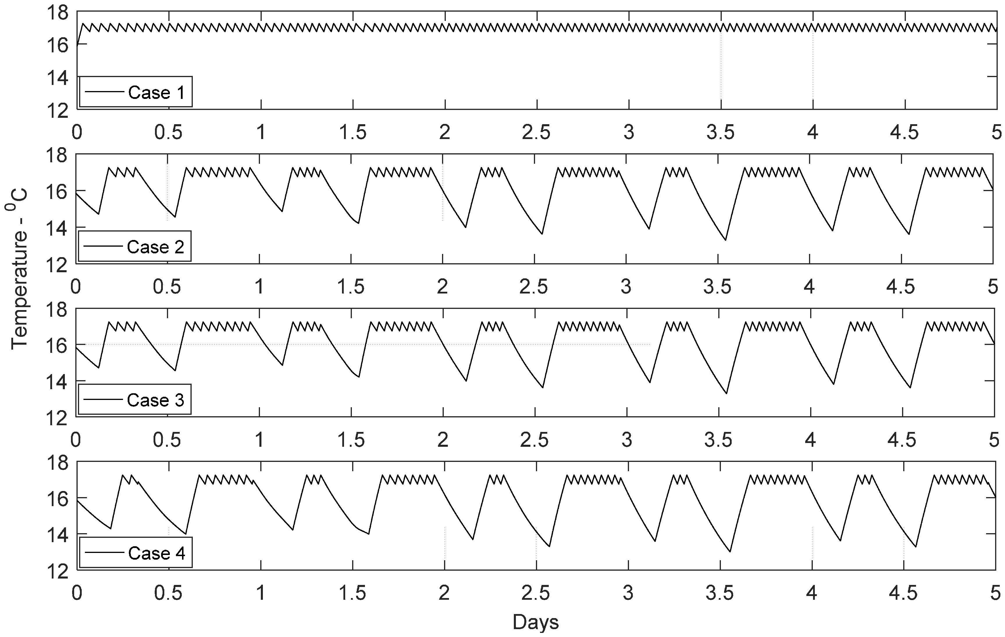
Figure 9.
Estimated heating times of the test building at the time of occupancy.

Figure 10.
Heater activity for Cases 1, 2, 3, and 4 based on the power supply from the heating system at each time instant.
Figure 10.
Heater activity for Cases 1, 2, 3, and 4 based on the power supply from the heating system at each time instant.

Figure 11.
Predicted temperature variation inside the test building for Case 5 and Case 6.

Figure 12.
Heater activity for Cases 5 and 6 based on the power supply from the heating system at each time instant. Graphs are given for both low set point temperatures of 12 °C and 5 °C.
Figure 12.
Heater activity for Cases 5 and 6 based on the power supply from the heating system at each time instant. Graphs are given for both low set point temperatures of 12 °C and 5 °C.
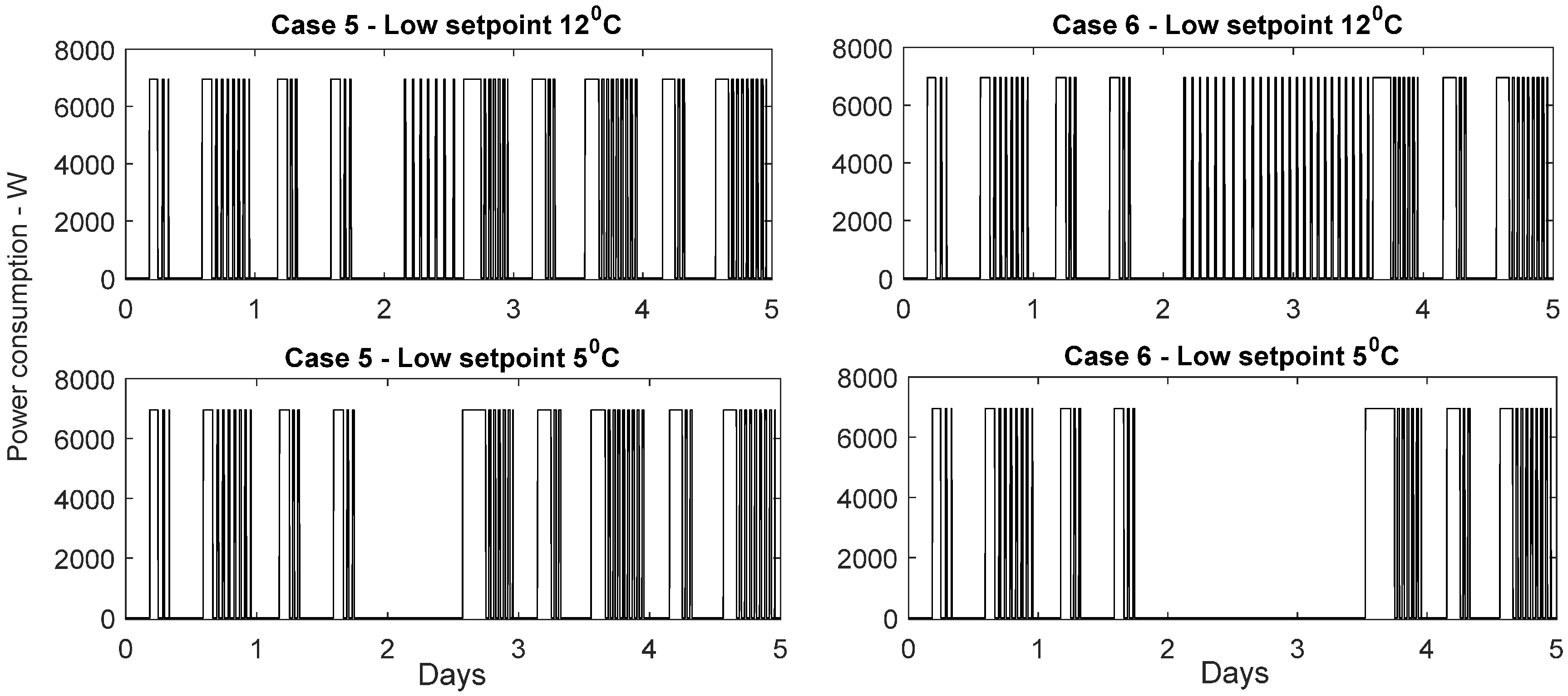
Figure 13.
Estimated space heating energy consumption for each case. Cases 5 and 6 are presented for both low set point temperatures of 12 °C and 5 °C.
Figure 13.
Estimated space heating energy consumption for each case. Cases 5 and 6 are presented for both low set point temperatures of 12 °C and 5 °C.

Table 1.
Description of the variables and parameters.
| Symbols | Description |
| A | Surface area [m2] |
| Specific heat capacity [J/(kg K)] | |
| E | Space heating energy consumption [kWh] |
| Specific enthalpy [J] | |
| M | Molar mass of air [kg/mol] |
| Air mass flow rate [kg/s] | |
| Heat flow rate [W] | |
| R | Gas constant [J/(mol K)] |
| T | Temperature [K] |
| x | Thickness [m] |
| U | Overall heat transfer coefficient [W/(m2K)] |
| V | Volume [m3] |
| α | Thermal diffusivity [m2/s] |
| ρ | Density [kg/m3] |
| t | Time [s] |
| η | Efficiency of the heat recovery system |
| δr | Thickness of a spherical layer/2 [m] |
| Subscripts | Description |
| app | Appliances |
| f | Floor |
| fur | Furniture |
| h | Heaters |
| i | Inside the building unit |
| j | jth layer |
| occ | Occupants |
| r | Roof |
| s | Solar irradiation |
| w | Wall |
| α | Outside environment |
| Superscripts | Description |
| s | Surface |
Table 2.
Calibrated parameters of the building heating model.
| Parameter | Attic |
|---|---|
| 1.2 × 10⁻⁷ m2/s | |
| 4.9 × 10⁻⁷ m2/s | |
| 4.6 × 10⁻⁷ m2/s | |
| 4.4 × 10⁻⁸ m2/s | |
| 0.1 W/(m2K) | |
| 0.9 W/(m2K) | |
| 0.15 W/(m2K) | |
| 2 W/(m2K) | |
| 1.7 W/(m2K) | |
| 1.2 W/(m2K) |
Table 3.
Estimated space heating energy consumptions for five days for each case.
| Case Number | Energy Consumption kWh |
|---|---|
| Actual | 249.4 |
| Case 1 | 291.9 |
| Case 2 | 261.4 |
| Case 3 | 261.4 |
| Case 4 | 252.5 |
| Case 5—12 °C | 234.5 |
| Case 5—5 °C | 229.3 |
| Case 6—12 °C | 208.5 |
| Case 6—5 °C | 178.1 |
© 2017 by the authors. Licensee MDPI, Basel, Switzerland. This article is an open access article distributed under the terms and conditions of the Creative Commons Attribution (CC BY) license (http://creativecommons.org/licenses/by/4.0/).
Share and Cite
MDPI and ACS Style
Perera, D.W.U.; Skeie, N.-O. Comparison of Space Heating Energy Consumption of Residential Buildings Based on Traditional and Model-Based Techniques. Buildings 2017, 7, 27. https://doi.org/10.3390/buildings7020027
AMA Style
Perera DWU, Skeie N-O. Comparison of Space Heating Energy Consumption of Residential Buildings Based on Traditional and Model-Based Techniques. Buildings. 2017; 7(2):27. https://doi.org/10.3390/buildings7020027
Chicago/Turabian StylePerera, Degurunnehalage Wathsala Upamali, and Nils-Olav Skeie. 2017. "Comparison of Space Heating Energy Consumption of Residential Buildings Based on Traditional and Model-Based Techniques" Buildings 7, no. 2: 27. https://doi.org/10.3390/buildings7020027
Note that from the first issue of 2016, this journal uses article numbers instead of page numbers. See further details here.