
Electrical Resistivity Tomography and Induced Polarization for Mapping the Subsurface of Alluvial Fans: A Case Study in Punata (Bolivia)


Abstract
:1. Introduction
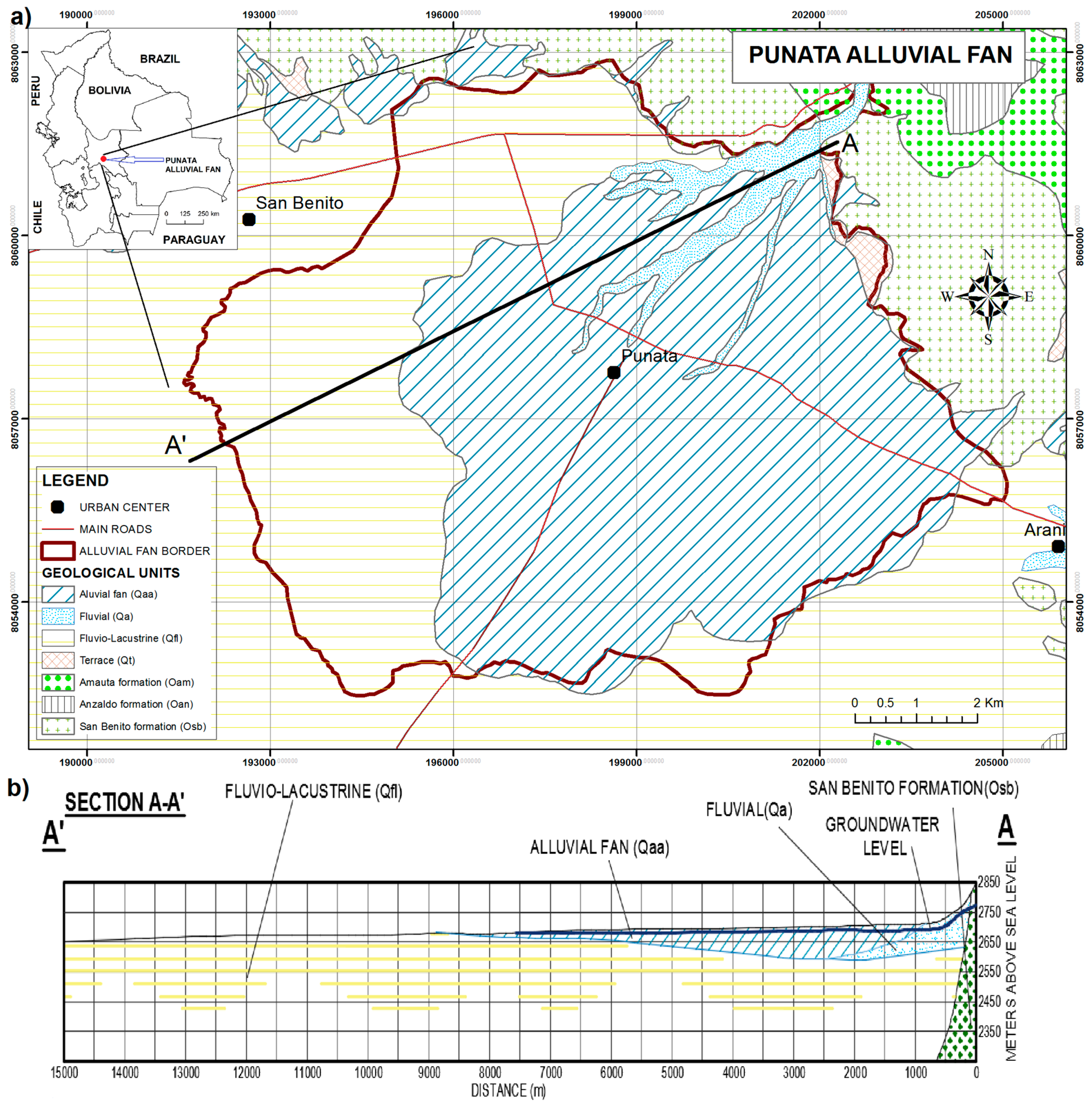
2. Study Area and Geological Settings
- Alluvial fan deposits (Qaa): Coarse grained materials, composed of boulders, gravel, and sand, forming alluvial fans and river channel deposits. Silt and clay are deposited in the top parts.
- Fluvial deposits (Qa): Boulders, gravel, and sand are the main materials which were transported and deposited by streams.
- Fluvio-lacustrine deposits (Qfl): Fine materials, consisting of clay and fine sand with intercalation of organic horizons and dark blue clays.
- Terrace deposits (Qt): Angular boulders of variable size, mixed with silt and sandy materials. These deposits cover the zones in the northeastern edge of the alluvial fan.
3. Methods
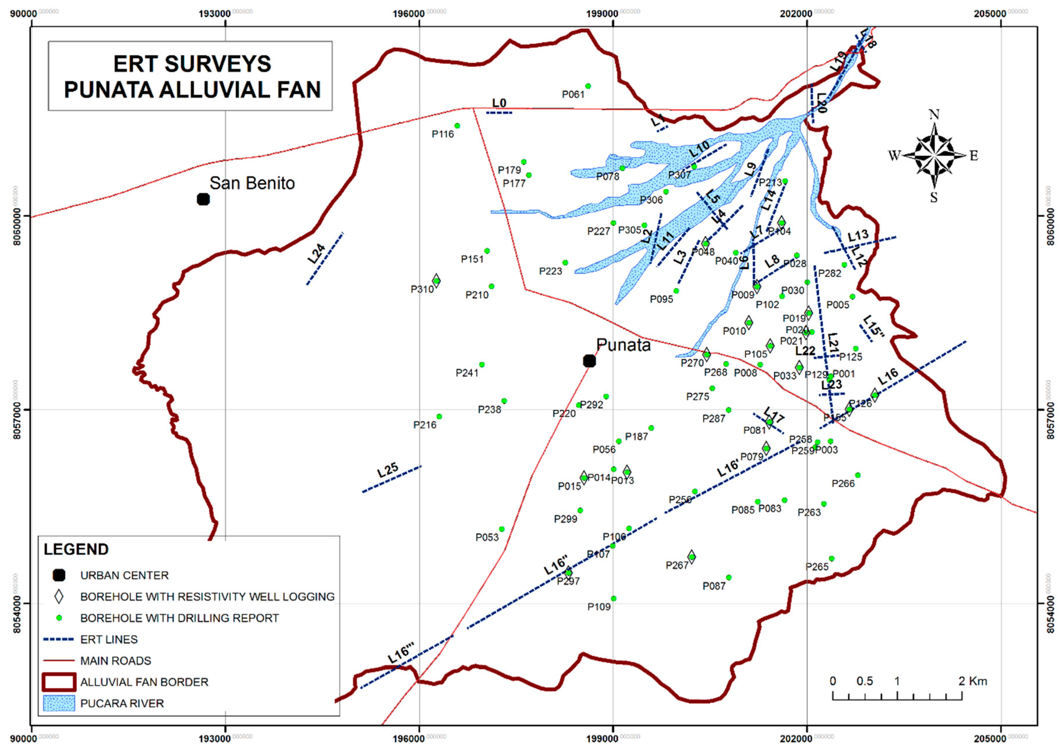
3.1. Data Acquisition
3.2. Data Processing and Inversion
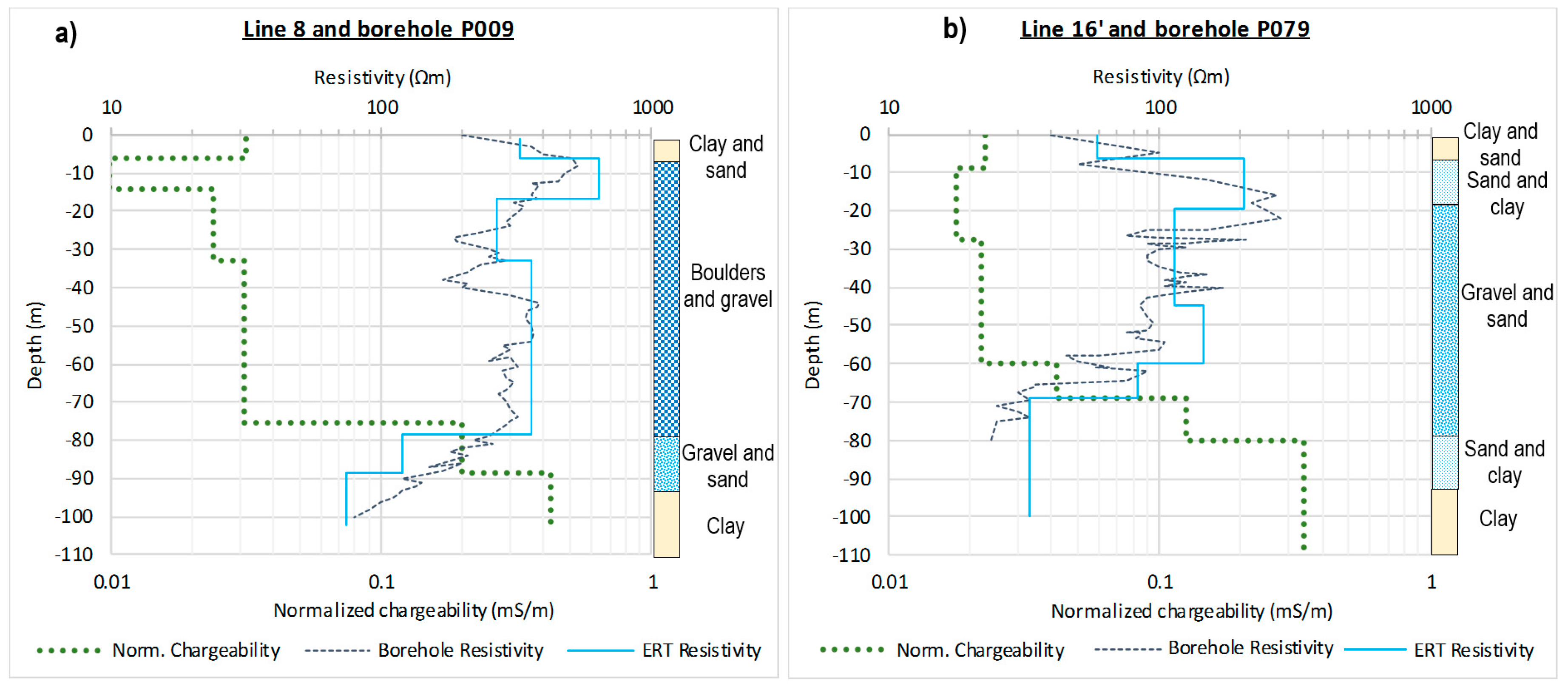
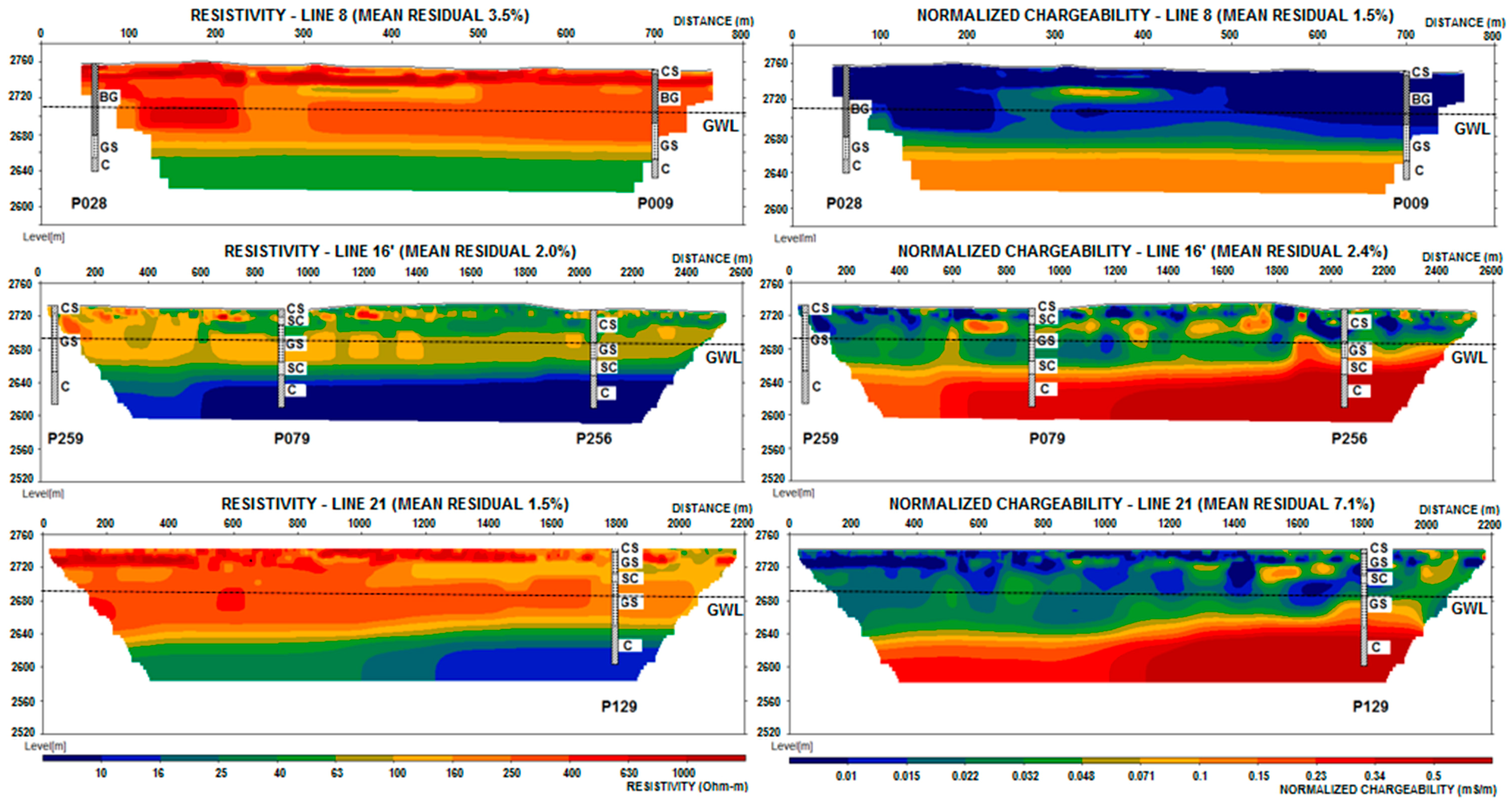
4. Results
5. Interpretation and Discussion
6. Conclusions
Acknowledgments
Author Contributions
Conflicts of Interest
Abbreviations
| ERT | Electrical resistivity Tomography |
| IP | Induced Polarization |
References
- Blair, T.C.; McPherson, J.G. Processes and forms of alluvial fans. Geomorphol. Desert Environ. 2009, 413–467. [Google Scholar]
- Blissenbach, E. Geology of alluvial fans in semiarid regions. Geol. Soc. Am. Bull. 1954, 65, 175–189. [Google Scholar] [CrossRef]
- Bridge, J.S.; Mackey, S.D. A Revised Alluvial Stratigraphy Model, in Alluvial Sedimentation; Blackwell Publishing Ltd.: Oxford, UK, 1993. [Google Scholar]
- Horton, B.K.; DeCelles, P.G. Modern and ancient fluvial megafans in the foreland basin system of the central Andes, Southern Bolivia: Implications for drainage network evolution in fold-thrust belts. Basin Res. 2001, 13, 43–63. [Google Scholar] [CrossRef]
- Bull, W.B. Recognition of Alluvial-Fan Deposits in the Stratigraphic Record; Society of Economic Paleontologists and Mineralogists: Tulsa, OK, USA, 1972; Volume 16, pp. 63–83. [Google Scholar]
- Martínez, J.; Benavente, J.; García-Aróstegui, J.L.; Hidalgo, M.C.; Rey, J. Contribution of electrical resistivity tomography to the study of detrital aquifers affected by seawater intrusion–extrusion effects: The river Vélez Delta (Vélez-Málaga, Southern Spain). Eng. Geol. 2009, 108, 161–168. [Google Scholar] [CrossRef]
- Baines, D.; Smith, D.G.; Froese, D.G.; Bauman, P.; Nimeck, G. Electrical resistivity ground imaging (ERGI): A new tool for mapping the lithology and geometry of channel-belts and valley-fills. Sedimentology 2002, 49, 441–449. [Google Scholar] [CrossRef]
- Arjwech, R.; Everett, M.E. Application of 2d electrical resistivity tomography to engineering projects: Three case studies. Songklanakarin J. Sci. Technol. 2015, 37, 675–682. [Google Scholar]
- Castilho, G.P.; Maia, D.F. A Successful Mixed Land-Underwater 3D Resistivity Survey in an Extremely Challenging Environment in Amazonia, Proceedings of the 21st EEGS Symposium on the Application of Geophysics to Engineering and Environmental Problems, Philadelphia, PA, USA, 6–10 April 2008.
- Dahlin, T. 2d resistivity surveying for environmental and engineering applications. First Break 1996, 14, 275–283. [Google Scholar] [CrossRef]
- Dahlin, T. The development of DC resistivity imaging techniques. Comput. Geosci. 2001, 9, 1019–1029. [Google Scholar] [CrossRef]
- Loke, M.; Dahlin, T. A comparison of the gauss–newton and quasi-newton methods in resistivity imaging inversion. J. Appl. Geophys. 2002, 49, 149–162. [Google Scholar] [CrossRef]
- Loke, M.; Lane, J.W., Jr. Inversion of data from electrical resistivity imaging surveys in water-covered areas. Explor. Geophys. 2004, 35, 266–271. [Google Scholar] [CrossRef]
- Loke, M.H.; Acworth, I.; Dahlin, T. A comparison of smooth and blocky inversion methods in 2d electrical imaging surveys. Explor. Geophys. 2003, 34, 182–187. [Google Scholar] [CrossRef]
- Crook, N.; Binley, A.; Knight, R.; Robinson, D.A.; Zarnetske, J.; Haggerty, R. Electrical resistivity imaging of the architecture of substream sediments. Water Resour. Res. 2008, 44, W00D13. [Google Scholar] [CrossRef]
- Marshall, D.J.; Madden, T.R. Induced polarization, a study of its causes. Geophysics 1959, 24, 790–816. [Google Scholar] [CrossRef]
- Magnusson, M.; Fernlund, J.R.; Dahlin, T. Geoelectrical imaging in the interpretation of geological conditions affecting quarry operations. Bull. Eng. Geol. Environ. 2010, 69, 465–486. [Google Scholar] [CrossRef]
- Sumner, J.S. Principles of Induced Polarization for Geophysical Exploration; Elsevier: Amsterdam, The Netherlands, 2012; Volume 5. [Google Scholar]
- Seigel, H.O. Mathematical formulation and type curves for induced polarization. Geophysics 1959, 24, 547–565. [Google Scholar] [CrossRef]
- Slater, L.D.; Lesmes, D. IP interpretation in environmental investigations. Geophysics 2002, 67, 77–88. [Google Scholar] [CrossRef]
- Alabi, A.A.; Ogungbe, A.S.; Adebo, B.; Lamina, O. Induced polarization interpretation for subsurface characterization: A case study of obadore, lagos state. Arch. Phys. Res. 2010, 1, 34–43. [Google Scholar]
- Revil, A.; Binley, A.; Mejus, L.; Kessouri, P. Predicting permeability from the characteristic relaxation time and intrinsic formation factor of complex conductivity spectra. Water Resour. Res. 2015, 51, 6672–6700. [Google Scholar] [CrossRef] [Green Version]
- Weller, A.; Slater, L.; Nordsiek, S. On the relationship between induced polarization and surface conductivity: Implications for petrophysical interpretation of electrical measurements. Geophysics 2013, 78, D315–D325. [Google Scholar] [CrossRef]
- Revil, A.; Florsch, N. Determination of permeability from spectral induced polarization in granular media. Geophys. J. Int. 2010, 181, 1480–1498. [Google Scholar] [CrossRef]
- Montenegro, E.; Rojas, F. Potencial Hidrico Superficialy Subterraneo del Abanico de Punata; Universidad Mayor de San Simon: Cochabamba, Bolivia, 2007. [Google Scholar]
- United Nations Development Programme-Servicio Geológico de Bolivia (UNDP-GEOBOL). Proyecto Integrado de Recursos Hidricos; Cordeco: Cochabamba, Bolivia, 1978. (In Spanish) [Google Scholar]
- Ahzegbobor, P.A. Assessment of soil salinity using electrical resistivity imaging and induced polarization methods. Afr. J. Agric. Res. 2014, 9, 3369–3378. [Google Scholar]
- SERGEOMIN. Mapa Geologico de Punata/Geological Map of Punata; SERGEOMIN: La Paz, Bolivia, 2011. (In Spanish) [Google Scholar]
- May, J.-H.; Zech, J.; Zech, R.; Preusser, F.; Argollo, J.; Kubik, P.W.; Veit, H. Reconstruction of a complex late quaternary glacial landscape in the cordillera de cochabamba (Bolivia) based on a morphostratigraphic and multiple dating approach. Quat. Res. 2011, 76, 106–118. [Google Scholar] [CrossRef]
- BRGM-SEURECA. Evaluacion de los Recursos de Agua y Abastecimiento en agua Potable de la Ciudad de Cochabamba, Bolivia; Semapa: Cochabamba, Bolivia, 1990. (In Spanish) [Google Scholar]
- Dahlin, T.; Zhou, B. A numerical comparison of 2d resistivity imaging with 10 electrode arrays. Geophys. Prospect. 2004, 52, 379–398. [Google Scholar] [CrossRef]
- Dahlin, T.; Zhou, B. Multiple-gradient array measurements for multichannel 2d resistivity imaging. Near Surface Geophys. 2006, 4, 113–123. [Google Scholar] [CrossRef]
- Kirsch, R. Groundwater Geophysics, 2nd ed.; Springer: Berlin/Heidelberg, Germany, 2009; Volume 1, p. 493. [Google Scholar]
- American Board of Electrodiagnostic Medicine (ABEM). Instruction Manual Terrameter LS; ABEM: Sundbyberg, Sweden, 2016. [Google Scholar]
- Loke, M. Res2dinv ver 3.59. 102. Geoelectrical Imaging 2D and 3D. Instruction Manual. Geotomo Software. 2010. Available online: http://www.geotomosoft.com/downloads.php (accessed on 14 November 2016).
- Nowroozi, A.A.; Whittecar, G.R.; Daniel, J.C. Estimating the yield of crushable stone in an alluvial fan deposit by electrical resistivity methods near Stuarts Draft, Virginia. J. Appl. Geophys. 1997, 38, 25–40. [Google Scholar] [CrossRef]
- Guérin, R.; Descloitres, M.; Coudrain, A.; Talbi, A.; Gallaire, R. Geophysical surveys for identifying saline groundwater in the semi-arid region of the central Altiplano, Bolivia. Hydrol. Process. 2001, 15, 3287–3301. [Google Scholar] [CrossRef]
- Perez, R. Estudio geoelectrico en el valle alto de rio paria. Geofis. Colomb. 1995, 1, 27–35. (In Spanish) [Google Scholar]
- Terrizzano, C.M.; Fazzito, S.Y.; Cortés, J.M.; Rapalini, A.E. Electrical resistivity tomography applied to the study of neotectonic structures, northwestern Precordillera Sur, Central Andes of Argentina. J. S. Am. Earth Sci. 2012, 34, 47–60. [Google Scholar] [CrossRef]
- Giocoli, A.; Magrì, C.; Vannoli, P.; Piscitelli, S.; Rizzo, E.; Siniscalchi, A.; Burrato, P.; Basso, C.; Di Nocera, S. Electrical Resistivity Tomography Investigations in the Ufita Valley (Southern Italy); Annals of Geophysics: Rome, Italy, 2008; Volume 51. [Google Scholar]
- Odudury, P.; Mamah, L. Integration of electrical resistivity and induced polarization for subsurface imaging around Ihe Pond, Nsukka, Anambra basin, Nigeria. Pac. J. Sci. Technol. 2014, 15, 306–317. [Google Scholar]
- Parkhomenko, E.I. Electrification Phenomena in Rocks; Springer Science & Business Media: Berlin/Heidelberg, Germany, 2013. [Google Scholar]
- Koch, K.; Revil, A.; Holliger, K. Relating the permeability of quartz sands to their grain size and spectral induced polarization characteristics. Geophys. J. Int. 2012, 190, 230–242. [Google Scholar] [CrossRef]
- Keller, G.V.; Frischknecht, F.C. Electrical Methods in Geophysical Prospecting; Road Research Laboratory: Osford, UK, 1966. [Google Scholar]


| Profile | Length (m) | Data Points | RMS Error (%) | Profile | Length (m) | Data Points | RMS Error (%) | ||
|---|---|---|---|---|---|---|---|---|---|
| Res. | I.P. | Res. | I.P. | ||||||
| L0 | 400 | 420 | 1.5 | 0.4 | L16’ | 2600 | 7215 | 2.0 | 2.4 |
| L2 | 800 | 509 | 3.0 | - | L16’’ | 3200 | 8812 | 6.9 | - |
| L4 | 800 | 1030 | 1.5 | 0.6 | L16’’’ | 1400 | 3272 | 5.2 | - |
| L5 | 800 | 952 | 3.5 | - | L17 | 600 | 1030 | 1.1 | - |
| L6 | 800 | 1030 | 5.3 | 6.0 | L18 | 200 | 457 | 2.7 | - |
| L7 | 800 | 752 | 3.4 | - | L19 | 1000 | 2073 | 2.1 | - |
| L8 | 800 | 1030 | 3.2 | 1.5 | L20 | 400 | 1120 | 5.8 | - |
| L12 | 800 | 1030 | 3.6 | - | L21 | 2200 | 6083 | 1.5 | 2.8 |
| L14 | 800 | 1030 | 1.8 | - | L22 | 400 | 512 | 1.3 | 7.1 |
| L15’’ | 100 | 431 | 4.7 | - | L23 | 400 | 512 | 1.5 | 2.3 |
| L15’’’ | 400 | 512 | 1.2 | - | L24 | 1000 | 1898 | 7.8 | - |
| L16 | 2400 | 6013 | 9.6 | - | L25 | 1000 | 1680 | 9.1 | 7.4 |
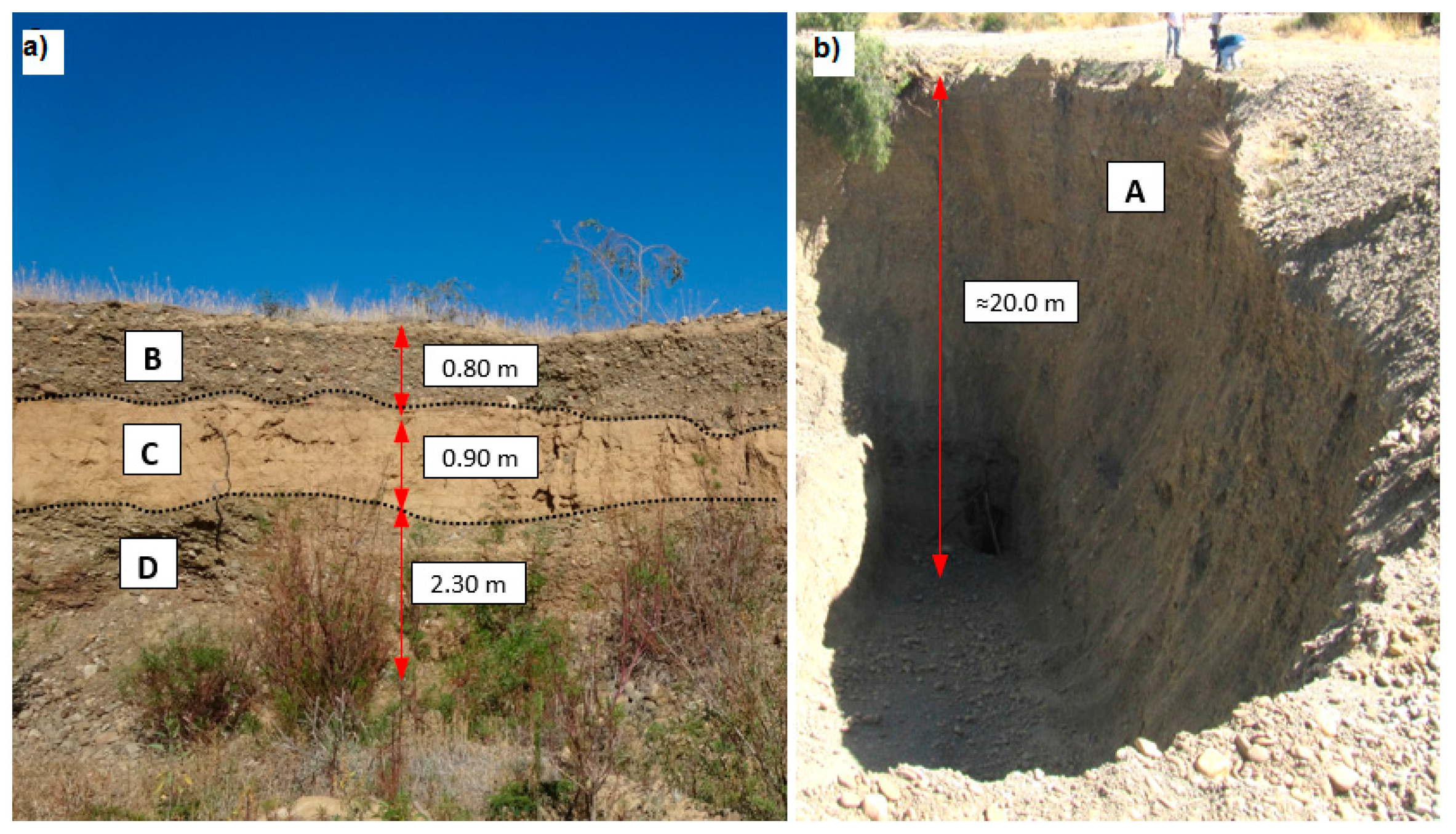
| Soil | Gravel (%) | Sand (%) | Silt (%) | Clay (%) | Bulk Density (g/cm3) | Particle Density (g/cm3) | Total Porosity (%) |
|---|---|---|---|---|---|---|---|
| A | 90.1 | 1.2 | 1.2 | 7.5 | 1.6 | 2.7 | 38.1 |
| B | 5.4 | 25.5 | 40.7 | 28.4 | 1.4 | 2.7 | 26.0 |
| C | 0.0 | 26.0 | 53.0 | 21.0 | 1.4 | 2.6 | 25.4 |
| D | 69.6 | 4.6 | 5.4 | 20.4 | 1.6 | 2.6 | 37.2 |
© 2016 by the authors; licensee MDPI, Basel, Switzerland. This article is an open access article distributed under the terms and conditions of the Creative Commons Attribution (CC-BY) license (http://creativecommons.org/licenses/by/4.0/).
Share and Cite
Gonzales Amaya, A.; Dahlin, T.; Barmen, G.; Rosberg, J.-E. Electrical Resistivity Tomography and Induced Polarization for Mapping the Subsurface of Alluvial Fans: A Case Study in Punata (Bolivia). Geosciences 2016, 6, 51. https://doi.org/10.3390/geosciences6040051
Gonzales Amaya A, Dahlin T, Barmen G, Rosberg J-E. Electrical Resistivity Tomography and Induced Polarization for Mapping the Subsurface of Alluvial Fans: A Case Study in Punata (Bolivia). Geosciences. 2016; 6(4):51. https://doi.org/10.3390/geosciences6040051
Chicago/Turabian StyleGonzales Amaya, Andres, Torleif Dahlin, Gerhard Barmen, and Jan-Erik Rosberg. 2016. "Electrical Resistivity Tomography and Induced Polarization for Mapping the Subsurface of Alluvial Fans: A Case Study in Punata (Bolivia)" Geosciences 6, no. 4: 51. https://doi.org/10.3390/geosciences6040051