Experimental Investigation of Debris-Induced Loading in Tsunami-Like Flood Events

Abstract

Debris loads during flood events have been well-documented by forensic engineering field surveys of affected communities. Research has primarily focused on debris impact loading and less emphasis has been placed into quantifying the loads and effects associated with debris damming, which occurs when solid objects accumulate at the front of structures. The formation of the debris dam has been shown to results in increased drag forces, backwater rise, and flow accelerations which can influence the stability of the structure. This study examined the formation of a debris dam in steady-state conditions of debris common to flood-prone communities. The study determined that the hydraulic conditions, in particular flow velocity, influenced the formation of the debris dam. Additionally, the study examined the influence of the blockage ratio on the backwater rise as well as the drag coefficient.

1. Introduction

Despite recent large-scale coastal flooding events, such as the 2004 Indian Ocean Tsunami, the 2005 Hurricane Katrina, and the 2013 Typhoon Haiyan, urban intensification of coastal regions has continued unabated [1,2]. Considering the increased potential for larger flood events as a result of climate change due to sea level rise and more extreme weather events [3], global population has become increasingly vulnerable to extreme coastal events. Consequently, there has been a focus on the development of comprehensive approaches for improving the preparedness, response, recovery, mitigation and protection of coastal communities for such extreme events [4].

One of the major problems when designing coastal protection infrastructure is the analysis of the loads and effects associated with these flooding events. Oftentimes, this includes research groups converging on the disaster-stricken coastal communities to measure and assess the damage and failure of the affected infrastructure. Forensic post-flooding field surveys, such as those of Ghobarah et al. [5] after the 2004 Indian Ocean Earthquake and Tsunami, Robertson et al. [6] after the 2005 Hurricane Katrina, and Naito et al. [7] after the 2011 Tohoku Earthquake and Tsunami, were conducted to collect post-disaster evidence and to investigate how structural failures may have occurred. In most cases, such surveys led to novel insights regarding structures that were thought to be capable of withstanding such extreme loading but still failed as a result of unforeseen or incorrectly estimated loads [8].

Across coastal events, one of the common loads which is difficult to assess, particularly in the context of post-flood field surveys, is debris loading [6,9,10]. Debris loads are a result of solid objects entrained within the inundating flow. Such debris can generally be separated into two categories: (1) direct debris impact; and (2) debris damming. Direct debris impacts are a dynamic load as a result of a floating, solid object striking a structure. Debris damming is often considered as a static load: they form as debris agglomerate onto the face of a structure resulting in increased loading due to a larger exposed area to the incoming flow.

Debris impact and debris damming have been examined within the context of steady and unsteady-state flow conditions [11,12,13,14,15,16,17]. Design debris impact loads have generally been described in literature as a solution to the 1-D bar problem, where an impulse load is exerted on a rigid structure [18]. Several approaches have been used in the solution of the 1-D bar problem within existing standards: impulse-momentum, work-energy, and contact stiffness [16]. Each solution requires a specific assumption related to one of the variables. Debris damming loads ($F_{dm}$) are often considered as an adjustment to the drag force equation associated with hydrodynamic forces, tending to act as a static load [19]:

$$F_{dm}=\frac{1}{2}{\rho }_w{C}_D{B}_{d}h{u}^2$$

(1)

where ${\rho }_w$ is the density of the fluid, $C_D$ is the drag coefficient (commonly taken as that used for a rectangular pier = 2.0), $B_d$ is the cross-stream width of the debris dam, $h$ is the water depth, and $u$ is the flow velocity.

While debris damming has not been extensively examined for the case of coastal flooding where non-stationary hydraulic conditions may uniquely govern the process of dam forming and build-up. Significant research has been conducted by hydraulic researchers investigating the formation of debris dams at bridge piers. Parola [20] prepared a report on the design of highway bridge piers resistant to debris damming loads. His study found that the drag coefficient was dependent on the blockage ratio (the fraction of the total unobstructed cross-section blocked by the debris dam) and on the Froude (Fr) number.

While the debris dam influences the loads exerted on a structure, the formation of the dam also can have secondary effects that must be considered in the design process. The constriction of the flow path results in backwater rise, potentially overtopping flood protection structures adjacent to those at the location of interest [21]. Debris dam-induced flow constrictions also causes flow accelerations underneath and downstream of the dam [22], which can result in significant scouring [23].

Fenton [24] used the conservation of momentum equations to calculate the increase of backwater levels due to the presence of obstacle in an open channel. The solution used a linear approximation of the momentum equation, making the proposed equation only applicable over a small reduction in momentum flux:

$$\Delta \eta =\frac{u^2}{2g}\frac{C_d}{\beta F{r}^2-1}\frac{a}{A}$$

(2)

where $u$ is the velocity of the fluid at the obstacle, $A$ is the cross-sectional area of the channel, $\beta$ is the Boussinesq coefficient and $a$ is the cross-section area of the obstacle transverse to the flow direction.

Schmocker and Hager [25] examined the formation of debris dams at a debris rack. The study examined the influence of opening size, debris density and debris volume. Schmocker and Hager [25] qualitatively showed the temporal evolution of the debris dam formation stayed relatively similar regardless of experimental conditions. The study also found the dam formation and backwater rise to be dependent on the Froude number as the dam tended to compact horizontally and be forced further into the cross-section of the flow at higher Froude numbers:

$$\frac{h}{V_D^{\frac{1}{3}}}=0.3F{r}^{0.3}$$

(3)

where $h$ is the backwater rise and $V_D$ is the volume of debris. Pagliara and Carnacina [26] examined the influence of debris dam roughness and porosity on scour profiles. Both the roughness and the porosity of dam had significant influence on the scour depth and final bed profile. Stancanelli et al. [27], in a study of stony debris flows at channel confluences, determined that a decreased dam porosity resulted in an increase in backwater rise.

The study of debris damming in tsunami-like flood events has not often been addressed. Pasha and Tanaka [28] examined the capture of debris at inland forests under steady-state flow conditions with a Froude number of 0.7. The study examined several different debris geometries and found that the capture mechanism varied based on the contact area with obstacles. Cylindrical debris, with the smaller contact area, tended to oscillate at the front of the structure forming less stable dams. Similar to Bocchiola [29], the capture efficiency was determined to decrease with increasing flow velocity and increase with debris length.

The objective of hydraulic research into debris damming has primarily focused on the effects associated with the formation of the debris dam. This study will examine the variables related to design considerations of coastal structures subject to extreme inflows: horizontal in-stream loads, associated drag coefficients and backwater rise. With the eventual intention to provide design consideration related to the design of coastal structures for debris damming loads in coastal flooding events, the objectives of this study are:

• Examine the influence of the supplied debris volume on the debris dam formation.
• Determine the influence of debris mixtures, based on the quantity and type of debris supplied, on debris dam formation.
• Evaluate the horizontal in-stream loads caused by the formation of a debris dam at the face of the structure.
• Examine the influence of debris dam properties such as non-structural void fraction and size on loads and backwater rise.

This study examines the influence of the debris properties, such as the volume of debris supplied to the dam and the properties of the dam, on debris damming loads at a generalized structure. The study predominately focuses on debris that are common to coastal communities, in the event of coastal flooding, as outlined by the ASCE7 Chapter 6—Tsunami Loads and Effects [30]. As mentioned earlier, current research has focused on the capture efficiency of specific hydraulic structures and the corresponding backwater rise. This study will focus on the associated loads and backwater rise as a function of the debris dam properties to aid in a more generalized approach for the variety of critical structures in coastal communities.

The paper is organized as follows: the “Experimental Setup” section describes the experimental facilities used at Waseda University, Japan, as well as the instrumentation and debris types; the “Results” section outlines the main findings of the study related to the debris dam formation, backwater rise, and associated loads; the “Discussion” analyzes the results in the context of the larger coastal engineering community and discusses potential scale effects; and finally, the “Conclusions” outline the results of the experiments in relation to the objectives indicated above.

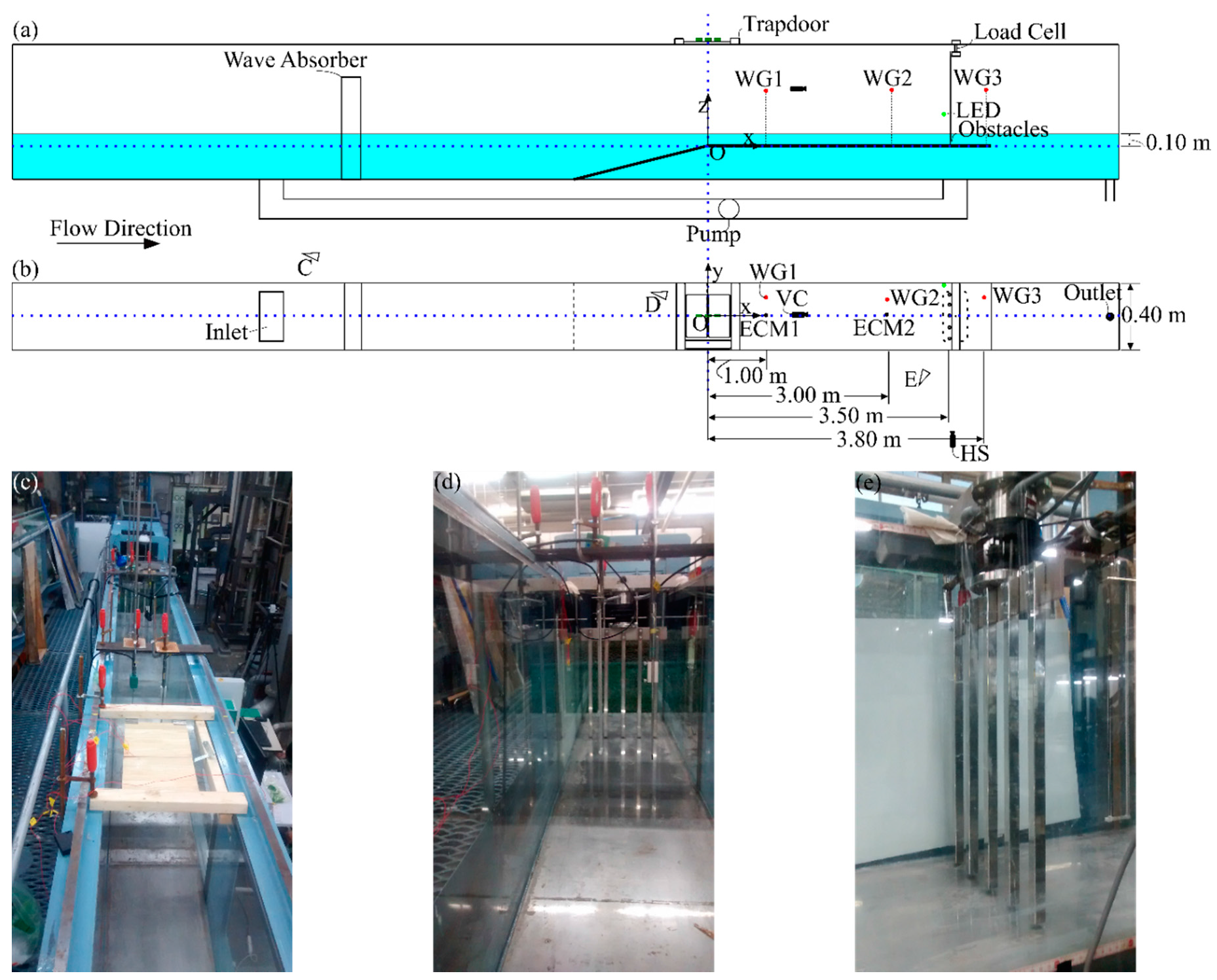
2. Experimental Setup

2.1. Experimental Facilities

Complex fluid–structure interaction between debris and a fixed obstacle governs the process of dam formation. Hence, experimental work is currently most promising to explore this problem at hand. As such, the experiments were performed at the High-Discharge Flume at Waseda University, Tokyo, Japan. The flume was 14.0 m long, 0.40 m wide and 0.80 m high (Figure 1) and is currently used for modeling 2D fluid problems. The experimental setup was placed on top of a 0.20 m false floor. The debris was released into steady-state flow conditions using a trapdoor placed on top of the flume (0.50 m from the water surface). The trapdoor opening was chosen to allow for all the debris to be released simultaneously for each experimental trial and improve repeatability. The debris were arranged on the trapdoor in the same manner for each experimental trial. The trapdoor was released and dropped into the steady-state flow. As each debris type was positively buoyant, the debris only briefly penetrated the water surface before surfacing and propagating in the flow direction. The origin of the experimental setup was considered to be on top of the false floor at the center point of the trapdoor, using a right-handed coordinate system with the flow direction as the positive x-direction (x) with the positive y-direction (y) flume left. The distance between the trapdoor and the obstacle was chosen based on Matsutomi [13] where the distance for the debris to reach steady-state flow velocity was 20 times the debris length, therefore giving the debris sufficient distance to reach steady velocity.

The obstacles to be impacted by the debris were modeled as a set of columns using a 1:50 length scale (Figure 2). The obstacles were modeled after structural columns in a building where breakaway walls had previously been destroyed by the inundating flow. The columns were 0.016 m wide with an opening width (W) of 0.06 m between each of the obstacles. The gap between the obstacles and the flume wall were 0.04 m on both sides and the obstacles were 0.40 m high. The width of the columns was chosen based on prescriptions from the National Building Code of Canada [31] corresponding to a general office building based on selected column spacing. The obstacles were placed 0.005 m above the bed surface to prevent them from touching the bed surface and thus influencing the force measurements from the load cell.

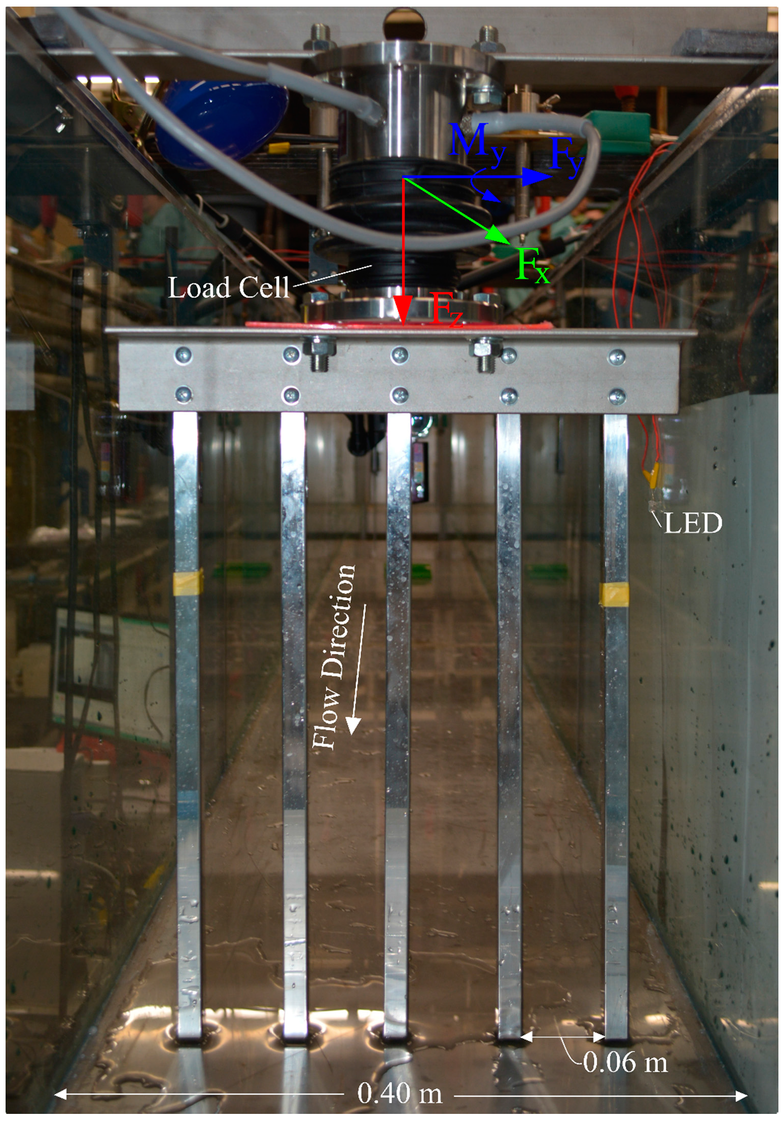
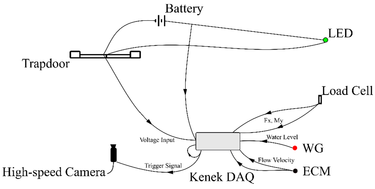
2.2. Instrumentation

The instrumentation setup is outlined in Figure 1 and

Table 1. Instrumentation used in experimental setup.

Instrumentation	Model	Instruments
Wave Gauge (WG)	KENEK CH-601	WG1, WG2, WG3
Electro-current Meter (ECM)	KENEK MT2-200	ECM1, ECM2
Video Camera (VC)	JVC Everio GZ-HM440
High-Speed Camera (HS)	KATO KOKEN k4
Load Cell (FT)	SSK LB120-50
Data Acquisition System (DAQ)	KENEK ADS2016

. The wave gauges (WG) were placed 0.10 m from the flume wall and the electro-current meters (ECM) were placed 0.20 m from the flume wall (center flume), 0.06 m from the bed. The WG and ECM were removed from the flume during the experiments containing debris to prevent damage due to accidental debris impact. The load cell was connected to the top of the obstacle setup, as shown in Figure 2. The load cell (FT) had a maximum rating force of 500 N, which exceeded any forces measured in these experiments. The load cell was calibrated by placing known weights along its three axis of coordinates. The load cell had a coefficient of calibration exceeding 0.99 for F_x, F_y and M_y. The FT was firmly connected to the top of the flume to ensure a rigid reference point. The sampling rate of all instruments was 100 Hz. The data from the FT were filtered using an Empirical Mode Decomposition (EMD) filter [32] to remove signal noise as well as the impulses caused by the debris impacting the structure. All the data from the hydraulic measurement equipment were collected into a single Data Acquisition (DAQ) system to assure synchronicity between the instruments.

Two cameras were setup to measure the formation of the debris dam. The video camera was placed upstream of the obstacles, facing the front face. The video camera (VC) recorded in an Advanced Video Coding High Definition (AVCHD) codec standard at 30 Hz. Before each experimental run, the video camera was manually triggered. The second camera was a high-speed camera (HS), commonly used in particle image velocimetry (PIV). The HS camera recorded each experiment using an Audio Video Interleaved (AVI) format at 100 Hz. The HS camera was manually triggered during the experiments.

As both camera systems were independent, a synchronization system was designed to minimize time discrepancies between the cameras and the DAQ recorded data (Figure 3). The trapdoor used to release the debris was connected to a simple circuit that, when broken, would turn off an LED light placed within the view of the video camera. Within each experimental video, the frame in which the LED light turned off would be considered as time zero. The voltage of the simple circuit was also input into the DAQ to indicate the time when the trapdoor was opened. The HS camera had a limited sampling window, therefore an output signal (5 V) was manually triggered by an operator as the debris approached the obstacles. The output signal triggered the HS camera to begin capturing images and the DAQ recorded the output signal to relate the trigger signal to time zero.

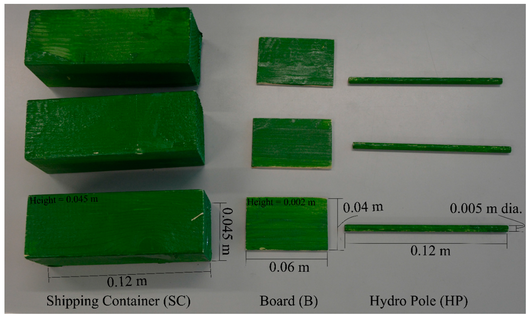
2.3. Model Debris

The debris were selected to model debris commonly found in coastal communities [30]. The experiments were scaled using a 1:50 length scale and were scaled geometrically using Froude similitude. Previous research on debris damming pertaining to debris mixtures is generally scarce with few exceptions, such as Schmoker and Hager [25], this work predominantly investigates mixtures of debris, as this is the most likely scenario for debris transported in an extreme flow condition in a coastal setting. Hence, three different types of debris were selected (Figure 4): shipping containers (SC), hydro poles (HP), and boards (B).

The debris were modeled after standard debris used in current building guidelines [30]. The properties of each debris type are outlined in

Table 2. Debris Properties.

Debris Properties	Dimensions					Dimensionless Variables
Type of Debris	Length (m)	Width (m)	Height (m)	Characteristic Length (m)	Surface Area-to-Volume Ratio (m−1)	Length (-)
Shipping Container (SC)	0.12	0.045	0.045	0.070	105.56	1.17
Hydro Pole (HP)	0.12	0.005	0.005	0.043	816.67	0.72
Board (B)	0.06	0.04	0.002	0.034	1083.33	0.57

and their geometry and aspect is shown in Figure 4. The shipping containers were modeled as standard 6.00 m long shipping containers [33]. The hydro poles were modeled as standard 6.00 m (0.25 m dia.) long hydro poles [11]. The boards were selected to model sheets of dry wall and plywood observed in images of debris damming that occurred in field studies [34]. The dry wall and plywood were generally of arbitrary shape as they were severely damaged when entrained within the flow; however, to maintain repeatability between cases, a single type of board (0.06 m × 0.04 m × 0.002 m) was selected.

The characteristic length is a variable often used to describe the physical properties of an object, however the definition varies widely depending on the application. As the focus of this study is on the formation of a debris dam, the primary factor influencing the dam formation is whether the debris contacts the obstacle or not. Visual observations of the debris propagation towards the obstacles showed that the orientation of the debris relative to the flow direction was a probabilistic process. Therefore, it was assumed that each dimension of the debris had equal chance of contacting the obstacles. Therefore, an average of the physical dimensions of the debris (length, width, and height) was used as the characteristic length. The characteristic length of the debris mixture was taken as the averaged characteristic length, weighed by the volume of debris present within each configuration. The dimensionless length (L) was the characteristic length of the debris divided by the opening width (W) of the obstacles.

$$L_c=\frac{V_{SC}{L}_{SC}+V_{HP}{L}_{HP}+V_B{L}_B}{V_{SC}+V_{HP}+V_B}$$

(4)

where V is the volume of the debris and $L$ is the length of the debris.

The debris was scaled using the 1:50 length scale for the dimensions and mass of the objects. However, due to the heterogeneous nature of prototype shipping containers and size-strength ratio of the boards and hydro poles, material properties (stiffness, yield strength, etc.) of the debris and the obstacles were not properly scaled [35]. Additionally, as shown in images from the 2005 Hurricane Katrina [6], significant damage affected the debris which could potentially influence the observed stability of the debris dam as well as the roughness of the dam within this study.

2.4. Experimental Protocol

As discussed in Section 1, this study aims to assess the influence of the debris concentration and flow velocity on dam formation and loads. The experiment employed three different flow velocities (0.3, 0.45, and 0.60 m/s), in combination with a large variety of debris configurations (

Table 3. Experimental Protocol.

Category	Experimental Condition	Water Depth (h) (m)	Flow Velocity (v) (m/s)	$\mathit{F}\mathit{r}=\mathit{v}/\sqrt{\mathit{g}\mathit{h}}$ (-)	Debris Cases (SC,HP,B)
1	A	0.10	0.60	0.60	0,0,0
2					9,0,0
3					0,81,0
4					0,0,20
5					3,27,7
6					7,9,2
7					1,63,2
8					1,9,16
9					6,54,14
10					9,81,20
11	B	0.10	0.30	0.30	0,0,0
12					9,0,0
13					0,81,0
14					0,0,20
15					3,27,7
16					7,9,2
17					1,63,2
18					1,9,16
19					6,54,14
20					9,81,20
21	C	0.10	0.45	0.45	0,0,0
22					9,0,0
23					0,81,0
24					0,0,20
25					3,27,7
26					7,9,2
27					1,63,2
28					1,9,16
29					6,54,14
30					9,81,20
31					1,0,0
32					0,103,0
33					0,0,52

). Within each experimental category, three repetitions were performed except in the case with the clear water conditions (Category 1, 11, and 21), for a total of 93 individual experiments. Three repetitions were chosen to examine the repeatability of each test case. Experiments were run for 60 s to allow for the dam to reach an equilibrium condition.

The experimental protocol was designed to fit within the framework of the risk associated with debris impact used in the ASCE7 Tsunami Loads and Effects [16,30]. The framework assesses the risk associated with debris impact as a function of the plan area of the debris. By extension, the occurrence of debris impact would also carry an associated risk of debris damming. As such, six cases were performed with similar plan area of the debris with different mixtures of the three debris types. Two cases were then performed with multiples of the plan area to evaluate the influence of the plan area. For the flow velocity of 0.45 m/s, three other experimental sets (31, 32, and 33) were performed to investigate the influence of the debris shape on the repeatability and loads associated with the dam formation by performing test with similar volumes.

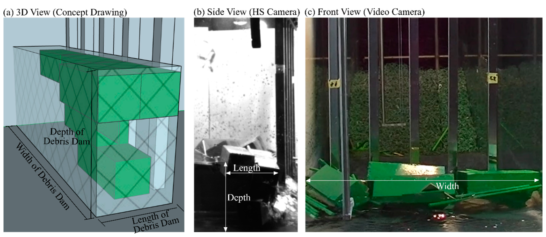
2.5. Debris Dam Measurement

The debris dam formation was monitored using the two-cameras setup shown in Figure 1. Due to difficulties with occlusion of sections of the dam from the side, as well as due to the 3D nature of the dam, the latter was conservatively defined as a uniform box related to its maximum width, depth, and length. The HS camera was used to monitor the depth (d) and length (l) of the dam (Figure 5b). To be consistent, the depth and length were selected based on the debris closest to the camera. The depth was considered for the free-surface water elevation at the structure to be consistent with the definition used for cross-sectional area of the debris dam in Equation (3). The video camera was used to monitor the width of the dam (Figure 5c). The width (w) was defined as the width of the debris dam at the face of the obstacles.

The dimensions of the dam were manually selected for each image within the experiment. Repetitions of four experimental trials found the standard deviation of the equilibrium dam length to be 0.01 m. Determining the correct debris dam shape could not be captured by the two camera system and there was not a system in place to capture such 3D images in a hydraulic environment due to potential for damage from the free-floating solid objects.

2.6. Statistical Analysis

Throughout the following section, statistical analysis is used to quantitatively determine the significance of the results. The following two tests, in particular, are used extensively and are explained within the context of this study. Through this section, the results of the statistical test are reported as the test statistic and p-value.

2.6.1. Paired T-Test

The paired t-test was used to examine the difference between the mean values between the different flow conditions. The basis of the paired t-test is to examine the change of a dependent variable between two related, independent groups [36]. The null hypothesis of the test states that the difference between each paired measurement is zero. For this study, the paired measurements are the mean value of the three repetitions for the various debris configurations.

2.6.2. Analysis of Covariance (ANCOVA)

The analysis of covariance is typically used to compare two or more regression lines to determine if the trends are significantly different [36]. The test is used to examine the change in a dependent variable between groups while controlling for the change in the variable as a function of a second measurement variable. The null hypothesis of the test states that both the slope and the y-intercept of the regression lines are statistically the same. For this study, the regression lines between the flow conditions were compared to determine if the flow conditions had a significant influence on the described results.

3. Results

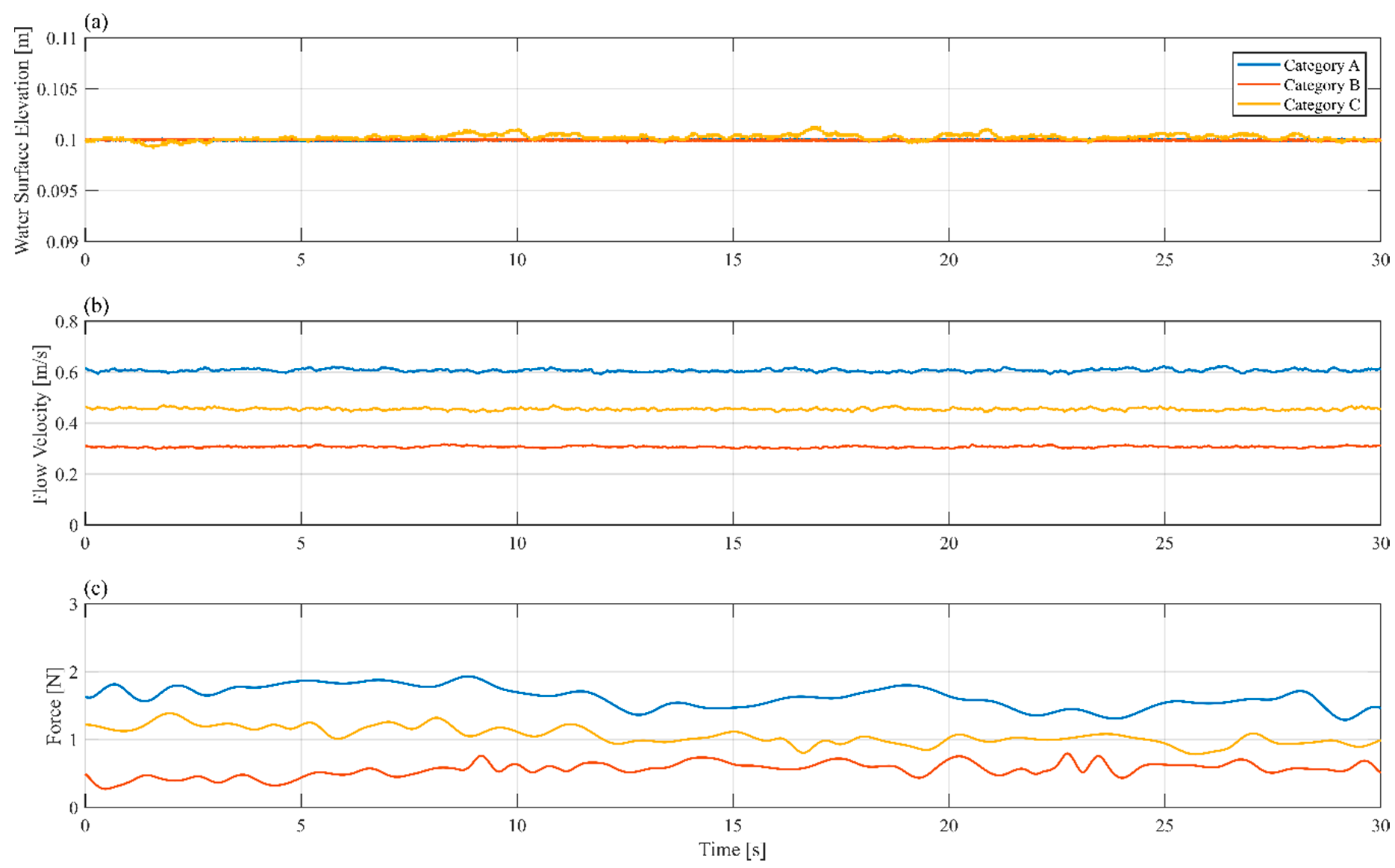
3.1. Experimental Hydrodynamics

Steady-state flow conditions were selected for the investigation of debris damming loads and effects due to the relatively long duration needed for the formation of an equilibrium debris dam condition [25]. Transient flow conditions often found during rapid coastal inundation events occurring as a result of storm surges or tsunami will be addressed in a separate study. Three flow velocities (0.30 m/s, 0.45 m/s, and 0.60 m/s) were selected for the experiments with a constant water depth. The time-history of the water depths, flow velocities and associated horizontal in-stream forces can be observed in Figure 6 for the clear-water conditions (no debris). As observed in Figure 6a,b, the flow was steady throughout this experimental run. The standard deviation from the mean, averaged across categories, was 2.91 × 10⁻⁴ m and 0.005 m/s for water heights (WG1) and flow velocity (ECM1), respectively.

The horizontal force measured in the flow direction (in-stream) for each clear water condition is shown in Figure 6c. The force measurement had a standard deviation of 0.203 N across the three categories. The rigid point, in which the load cell was connected to the flume wall, was also connected to the pump. As a result, slight vibrations were noted; however, the resulting noise was negligible. For each category, the mean drag coefficient per unit width was calculated for the entire obstacle as 0.60 ± 0.057 (95% Confidence Interval (CI)).

While it is widely established that coastal flooding events are characterized by transient flow conditions, there are significant difficulties in physically modeling the long duration flow events, particularly in the case of tsunamis [37]. As a preliminary investigation of debris damming, the transient nature of coastal flooding was not considered herein. However, comparing to tsunamis, the time scale of the local flow conditions, in field studies of tsunami-stricken areas, (~7 min at prototype scale) is significantly shorter than the tsunami wave period (>10 min) [38]. The flow velocities at prototype scale (2–7 m/s) in these tests compared well to the velocities observed in the 2004 Indian Ocean Tsunami (2–5 m/s) [39].

The drag coefficient varies with the Reynolds number in incompressible flow [40]. As the experiments were scaled using Froude similitude, scale issues potentially exist. Bricker et al. [41] outlined the necessity for properly scaling the Reynolds and Weber numbers to correctly address issues related to turbulence and surface tension. The experiment presented herein had Reynolds numbers in the range of 3–6 × 10⁵, representing the fully turbulent flow condition needed to avoid significant scale effects. Additionally, the Weber number ranged from 123.6–494.5 which exceeds the critical values of 120 presented by Peakall and Warburton [42].

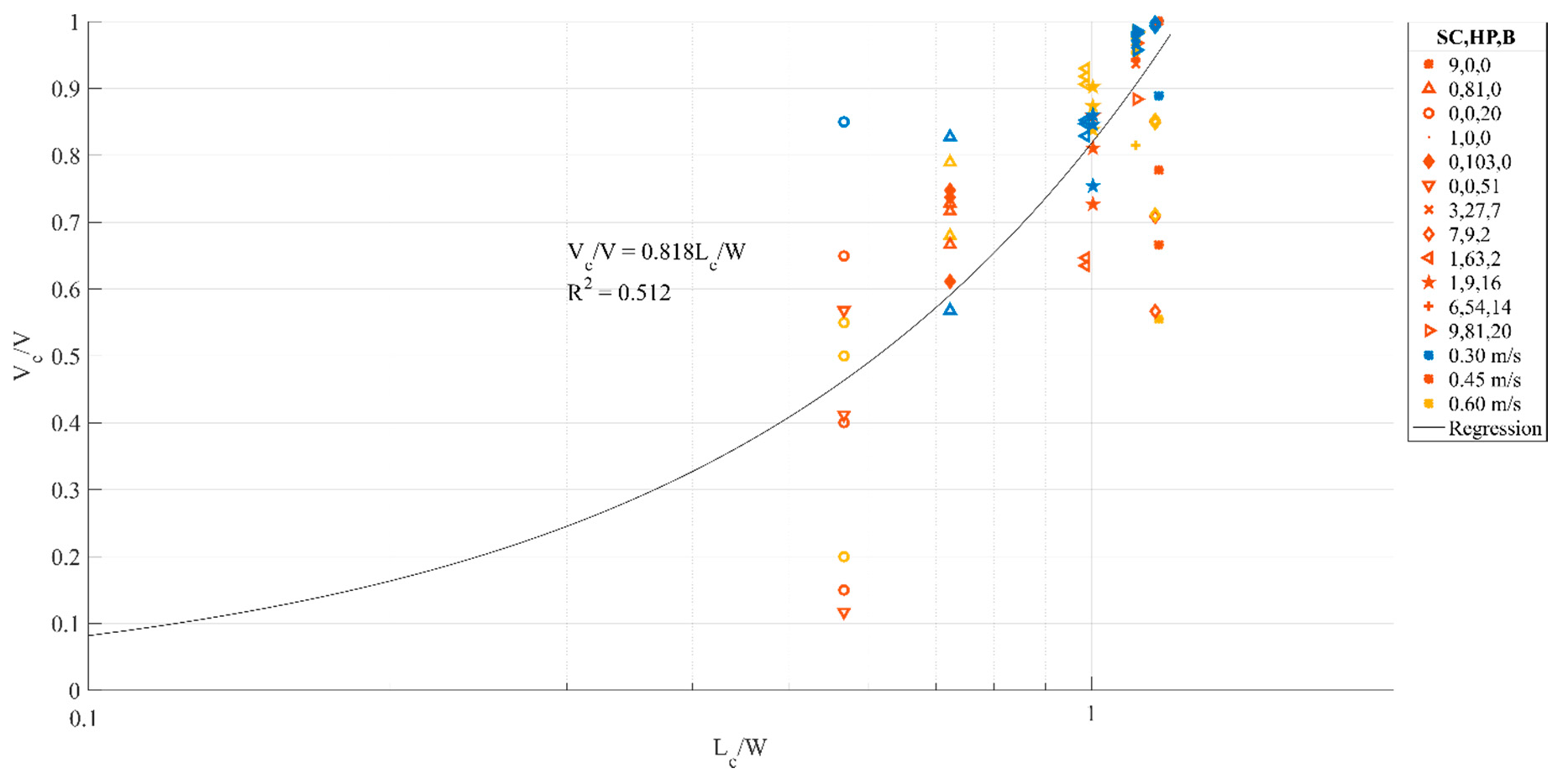
3.2. Debris Geometry

To examine the influence of the debris geometry, three experimental categories were conducted with the same volume of debris (categories 31, 32, and 33). While each case resulted in an increase in the forces acting on the obstacles, there was noticeable deviation in the magnitude and repeatability of the equilibrium force condition. Figure 7 shows the difference in force–time histories for each of the same volume cases and compares with the base case where not debris was added into the water.

The differences in the debris geometry resulted in varying dam formation characteristics. The cases with a single shipping container consistently formed a dam with similar characteristics and loads, whereas the characteristics of the hydro pole and boards varied between trials. Bocchiola et al. [38] discussed the importance of the “key” log in the formation of a debris dam. The “key” log refers to the first object to get caught on the obstacle and initiates the formation of the dam.

The formation of the “key” log influenced the deviations observed in the force–time histories. The case with the single shipping container consistently resulted in the dam forming as the length of the shipping container exceeded the width between the obstacles. Similarly, the hydro pole length exceeded the distance between the obstacles; however, the smaller characteristic length (a function of the dimensions of the debris) resulted in larger deviation between trials. The boards’ length was equal to the distance between the obstacles, resulting in the board being unable to bridge between two obstacles and an inconsistent formation of the dam.

A comparison of the capture efficiency (the number of debris capture divided by the total number of debris) for each debris type for all the experiments (regardless of debris mixture) shows the influence of the physical properties of the debris (Figure 8). The probability in this case was the count of the number of experiments divided by the number of experiments that contained the debris type. The mean capture rate (average percentage of each type of debris captured in the experiment) and standard deviation (SD) are shown on each histogram. Due to the larger size of the shipping container, the debris was consistently captured with a significantly greater capture rate and less deviation, whereas the smaller characteristic length of the hydro poles and boards resulted in smaller capture rates with greater deviation between experiments.

The difference in the magnitude of the load as a result of the debris dam formation was a function of the blockage ratio (B) caused by the debris dam (the area of the dam transverse (a) to the flow direction divided by the total available cross-section of the flow (A)). While each case depicted in Figure 7 had the same volume, the hydro poles and boards had an increased available surface area due to their increased surface area-to-volume ratio. Therefore, for a given volume of debris and flow condition, the characteristic length of the debris influenced the consistency of the formation of the dam and the surface area-to-volume ratio influenced the magnitude of the debris damming load.

3.3. Debris Dam Properties

The formation of a debris dam has been well-established by Bocchiola et al. [29] and Schmocker and Hager [25]. The initial formation of the dam begins once the “key” log has become blocked at the obstacle face (Figure 9a). The initial formation results in the streamlines forcing the incoming debris to begin to span the width of the flume (y-direction) (Figure 9b) [25]. As the debris continue to accumulate on the face of the obstacle (increasing the width of the dam), the power of the flow causes the dam to compact at the obstacle face, forcing the debris at the face towards the flume bottom (increasing the depth of the dam) (Figure 9c). Throughout this process, the dam continually increases the blockage of the flow, causing a rise in water level (backwater rise) and a reduction in the flow velocity. Once the flow velocity has been sufficiently reduced, a debris carpet begins to form upstream of the dam (increasing the length of the dam) (Figure 9d).

Pfister et al. [39] showed that the capture efficiency was dependent on the diameter (D) of the debris, in this case large woody debris, for a piano key weir. Their study showed that the capture efficiency of the large woody debris was high when the diameter was greater than 1.

$$\frac{V_c}{V}=1.5\left(\frac{D}{W}\right)-0.5$$

(5)

Figure 8 shows the individual debris capture efficiency for each experiment. Figure 10 shows the capture efficiency of each experiment based on the volume-averaged dimensionless length. As can be observed, the capture efficiency approximately linearly increased as the characteristic length increased (R² = 0.512):

$$\frac{V_c}{V}=0.818\frac{L_c}{W}$$

(6)

where $V_c$ is the captured volume of debris at the obstacle face and $V$ is the total volume of debris. An ANCOVA comparison of the trends for the different flow conditions showed no significant difference between the capture efficiency regression lines (F (2,81) = 0.45, p = 0.641). Previous studies indicated with increased Froude number, the stability of dam decreased [29], however this was not observed in this study, potentially due to the relatively small range of Froude numbers examined.

Equation (6) represents a deterministic evaluation of the volume capture as a function of the dimensionless characteristic length. However, as discussed earlier, debris transport is a stochastic process. The propagation orientation of the debris, which influenced weather the debris would contact the obstacle or not, is a probabilistic process influenced by a variety of factor, such as the flow conditions and surrounding topography [29]. As a result, significant scatter can be observed around the regression line. In this study, the characteristic length was calculated assuming that each side had an equal opportunity of forming the “key” log. Previous studies of debris transport have discussed the prevalence of a mean orientation [17] around which the likely debris orientations within the flow would be distributed. Detailed stochastic analysis of solid object orientation within the flow is needed to get a more accurate estimation of the characteristic length, something that is outside the scope of this study.

Figure 11 shows the formation properties of the dam, namely its width, length, and depth as a function of the debris volume. As expected, all properties of the dam increased with an increase in the debris supply. In this study, the width of the dam was limited by the flume width (0.40 m). Similarly, the depth of the debris dam was limited by the flume bottom; however, this limitation was offset by the increasing flow depth as a result of flow blockage. This resulted in dam depths potentially greater than the initial flow depth. The debris length was influenced by the flow velocity as sufficiently high flow velocities would cause the dam to compact at the obstacle face as opposed to forming the debris carpet.

A comparison of the dam formation with the differing flow velocities further confirms the dam formation process outlined by Schmocker and Hager [24]. In the cases with the larger flow velocity, compaction of the dam at the face of the structure occurred, forcing the debris towards the bed. As shown in Figure 11c, the cases with the larger flow velocities consistently had larger depths. Additionally, the cases with lower flow velocities resulted in the dam lengthening as the debris carpet formed, and, alternatively, shallower dams. The width of the debris dam appeared to be primarily driven by the amount of debris supplied to the obstacle.

Additional considerations are needed when addressing the formation of the dam in coastal settings. Pasha and Tanaka [40], in their study of debris damming in coastal forests during a tsunami event, found that debris with a larger surface contacting the structure were more stable and less likely to be forced towards the bed. In Figure 11, cases with larger volumes of the hydro poles (circle and star markers) tended to form deeper dams as a result of less contact area with the obstacle, whereas the boards and shipping containers tended to contact the obstacles and become immediately stable forming shallower dams.

Considering Equation (1), an important aspect of the debris dam governing the debris loads is the transverse cross-sectional area of the dam. In the case of this study, the transverse cross-sectional area was designated by the width and depth. As the flow velocity influenced the formation of the dam, Figure 12 shows the cross-sectional area (a), normalized by the available cross-sectional area ($A$), herein referred to as the blockage ratio (B), as a function of the Froude number.

$$B=\frac{a}{A}$$

(7)

As the width of the debris dam was primarily determined based on the volume of debris supplied to the site, increasing the Froude number resulted in deeper dams. Figure 12 shows an increase in the mean blockage ratio as a function of the Froude number. A paired t-test was performed between the three flow velocities and found significantly greater blockage ratio as the Froude number increased. Between Froude numbers of 0.3 and 0.45, the blockage ratio was significantly greater (t(8) = −2.805, p = 0.023) and similarly for Froude numbers between 0.45 and 0.6 (t(8) = −3.278, p = 0.0112).

As shown in Figure 12, there was significant deviation in the cross-section of the dam. Considering the random nature associated with debris motion [13,42], the formation of the “key” log varied between experimental cases which influenced when the dam began to form and the amount of debris trapped within it. The increased Froude number additionally resulted in increased stability of the initial “key” log, which aided in the formation of the dam. While the porosity of the dam could not be established in this study, the increase compaction of the dam caused by the increased flow power would decrease the porosity of the dam. However, further research is needed to evaluate the extent of this influence.

While general observations can be made regarding the dam formation, the relatively small width of the flume resulted in a limit to the dam formation influencing the effectiveness in developing comprehensive methods of estimating dam size from debris volume and flow conditions. Additionally, due to difficulties in directly assessing the cross-sectional area, the selection method was conservative, as it did not consider the porosity of the dam.

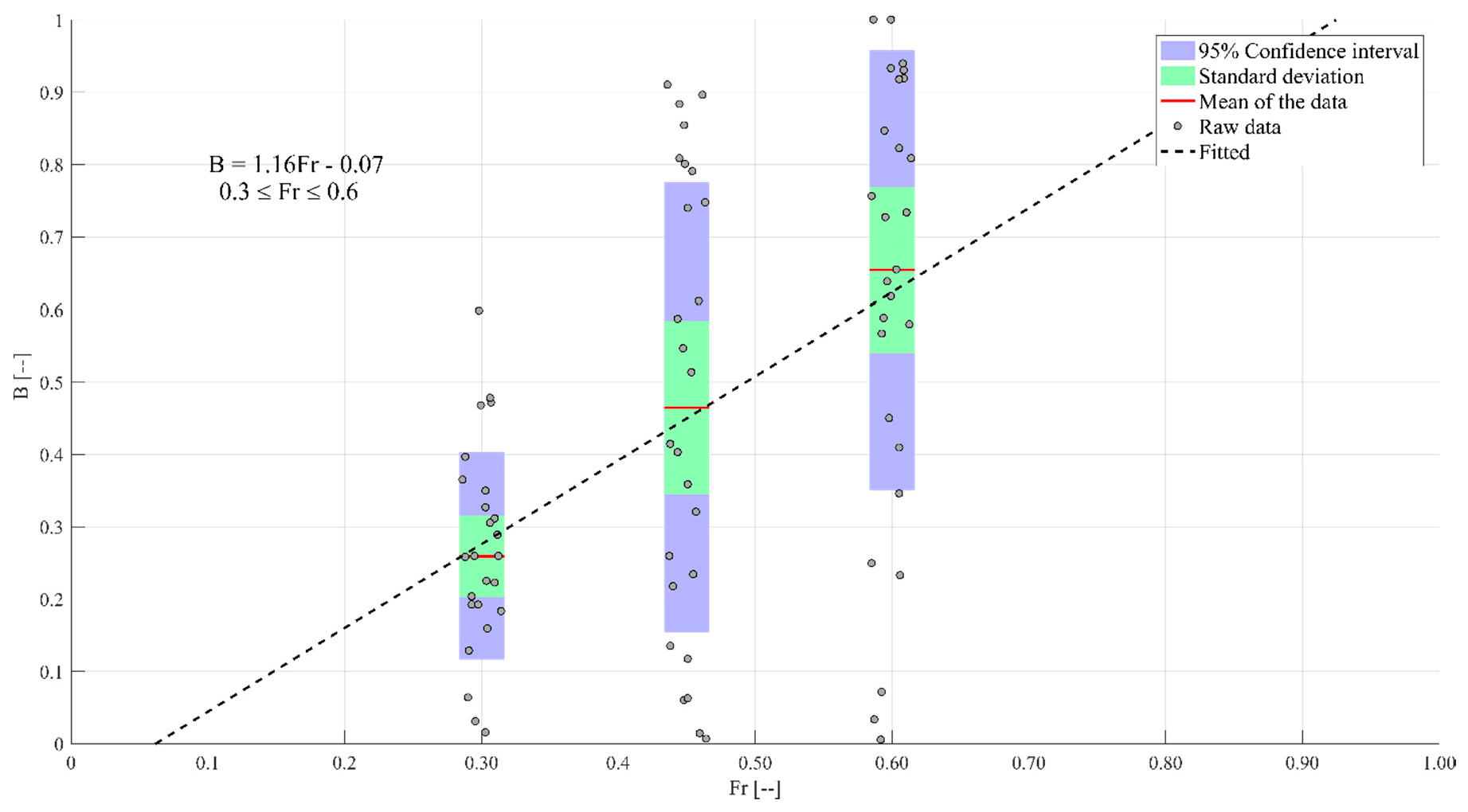
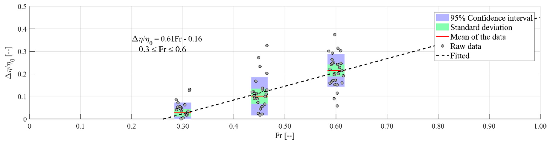
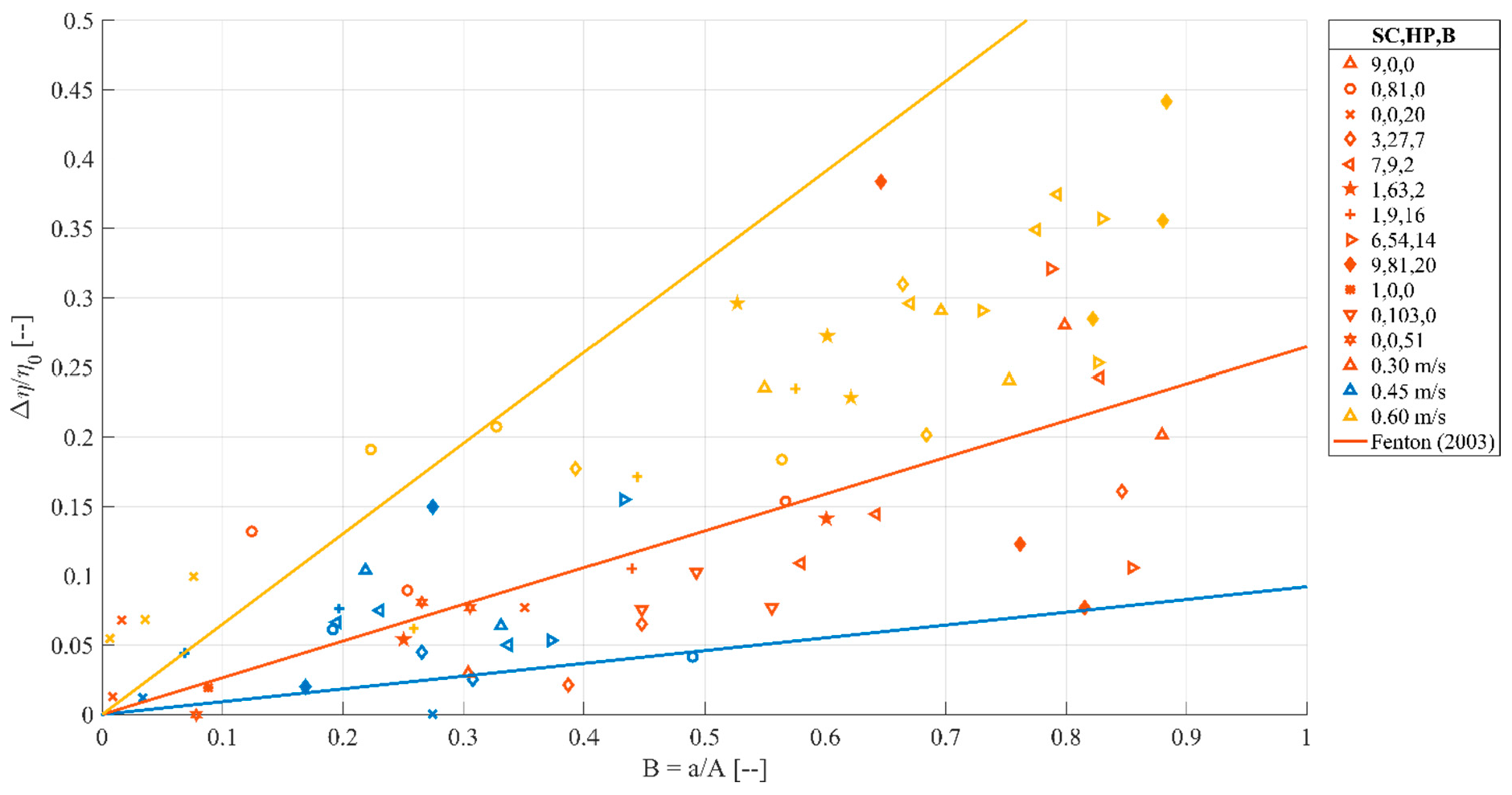
3.4. Backwater Rise

The application of the energy equations across an obstruction in a channel in subcritical flow conditions shows that a corresponding increase in the channel constriction results in a rise of the water surface upstream of the obstruction [43]. In the context of this study, backwater rise ($\Delta \eta$) is defined as:

$$\frac{\Delta \eta }{{\eta }_0}=\frac{\eta -{\eta }_t}{{\eta }_0}$$

(8)

where ${\eta }_0$ is the initial water level without the obstacles (for all cases 0.10 m), $\eta$ is the water level upstream of the dam, and ${\eta }_t$ is the water level without the dam (as a result of the obstruction of the obstacles).

Using the momentum equations (Equation (2)), Fenton [23] showed that backwater rises as a function of the Froude number. Figure 13 displays the backwater rise, normalized by the initial water depth, as a function of the Froude number. The backwater rise showed a significant increase as the Froude number increased as expected due to the increase in the blockage ratio. Between a Froude number of 0.3 and 0.45, the backwater rise increased (t(8) = −5.433, p < 0.001) as well as between 0.45 and 0.6 (t(8) = −6.764, p < 0.001).

Figure 14 shows a comparison of the backwater rise in the experiments to the analytical solution from Fenton [23]. A constant drag coefficient was used, estimated in the following section for the cases where blockage ratios (B) exceed 0.46 (C_D = 1.417). The analytical solution well represents the trend of the backwater rise, however tends to overestimate the magnitude. Fenton [23] noted that the linear explicit approximation of the momentum across the obstruction used in Equation (2) would only be valid over a small obstruction of the channel, as large obstructions were generally observed this potentially resulted in the discrepancy. Additionally, Schmocker and Hager [25] noted that the Froude number and available volume of debris influenced the backwater rise by influencing the compaction of the dam. This is particularly significant as the blockage of the dam was conservatively estimated. Additionally, porosity and irregular shapes were not considered in the calculation of the cross-sectional area of the dam.

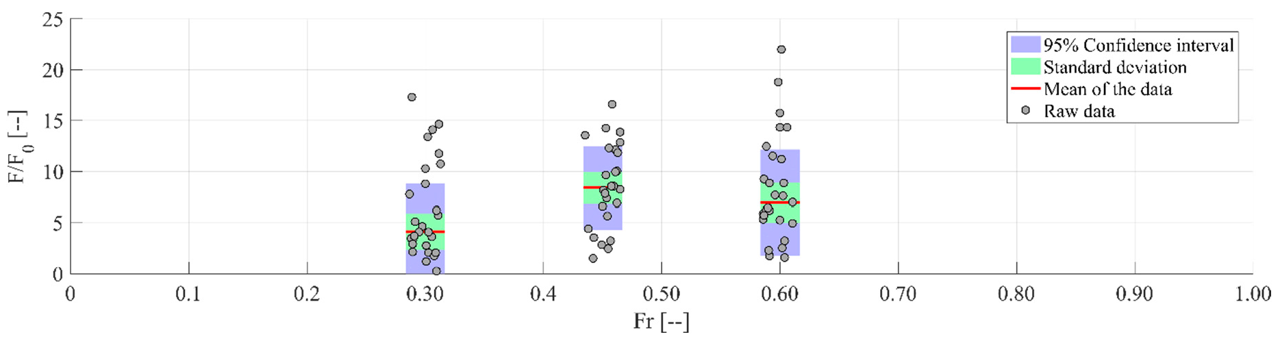
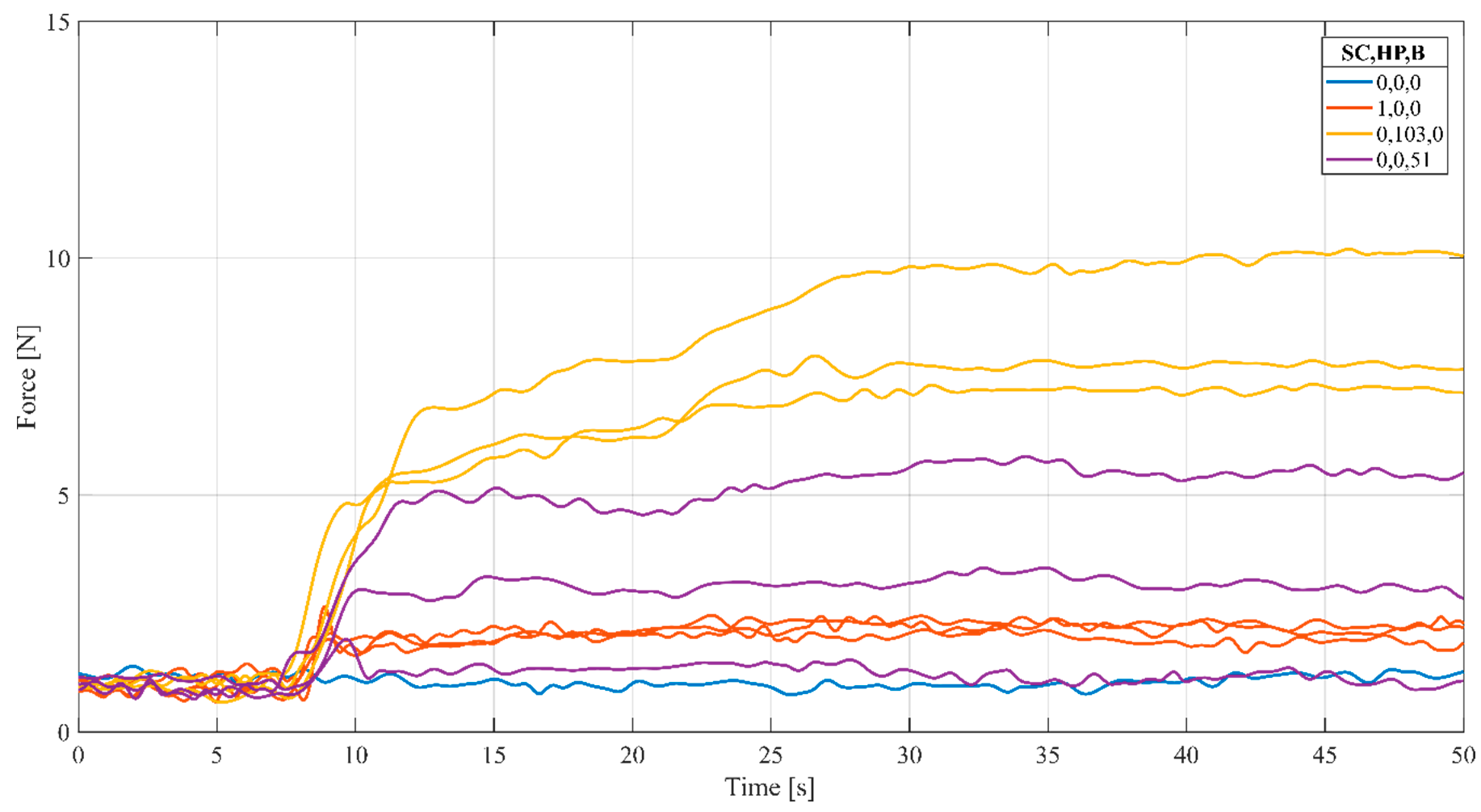
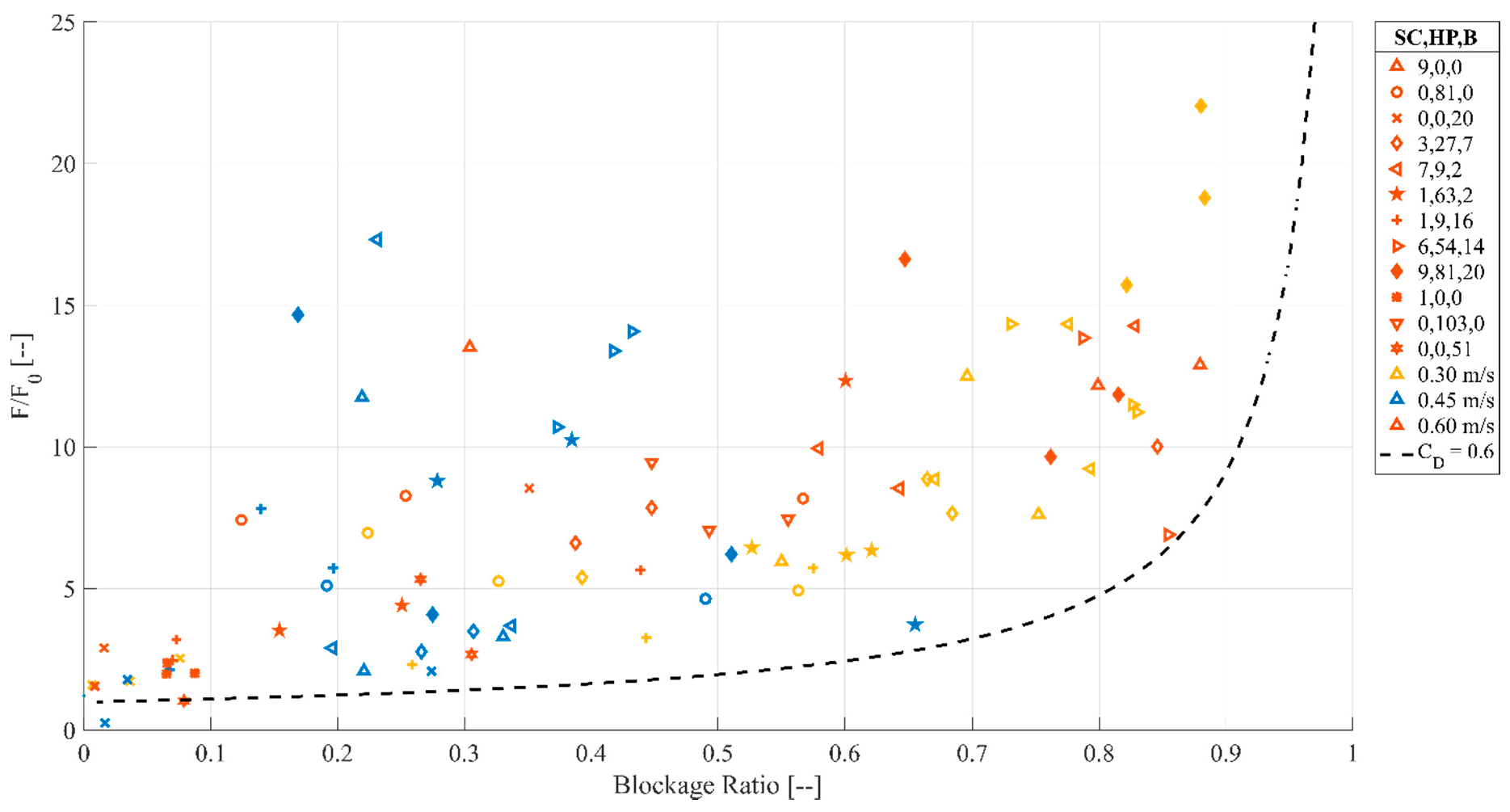
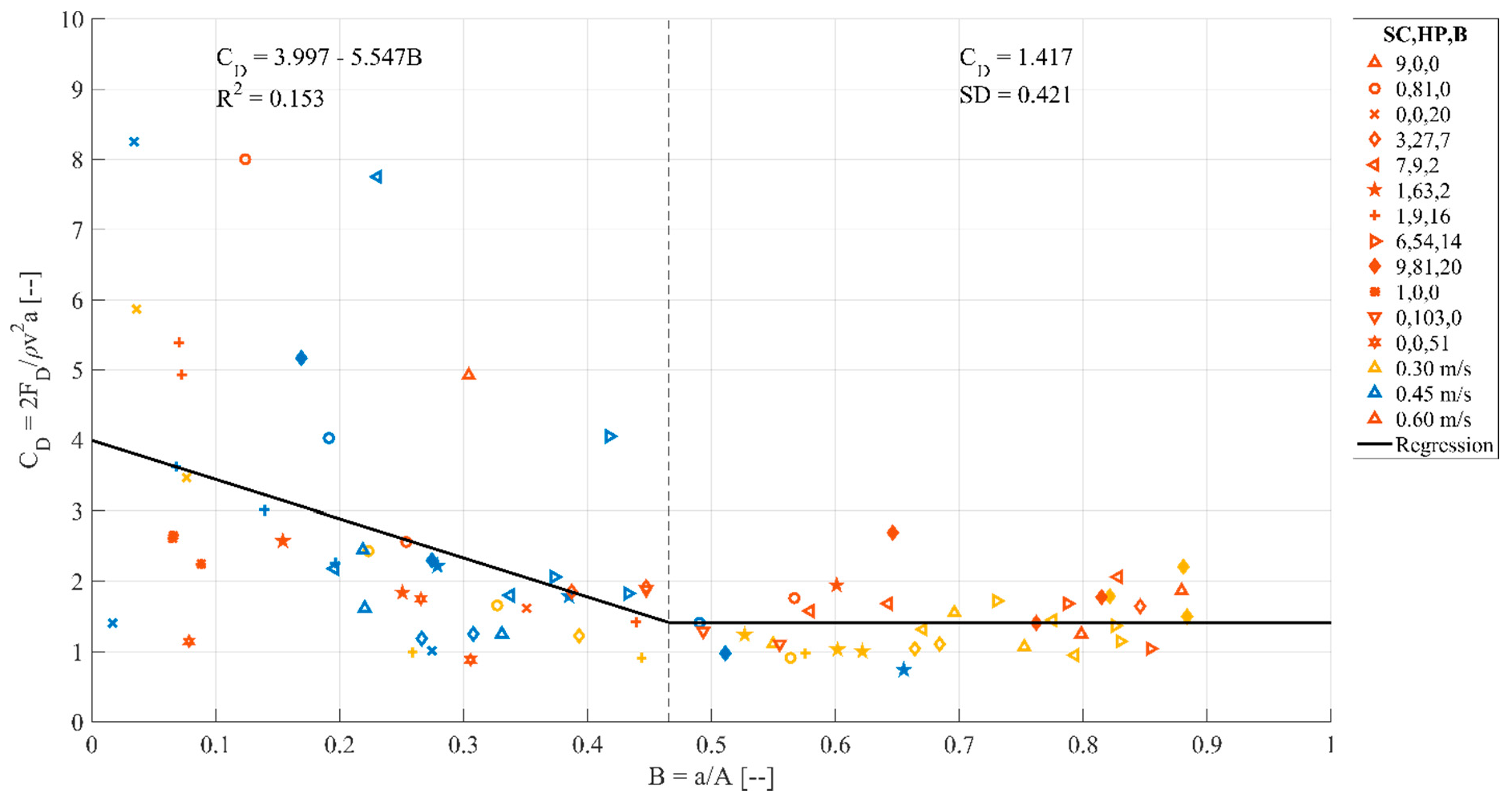
3.5. Drag Forces

As discussed in Section 1, debris damming has often been discussed within the context of increase drag forces acting on the obstacles. As can be observed from Equation (1), the drag force is a function of the exposed cross-section area and the drag coefficient. A comparison of all the experiments showed than an increase in the Froude number resulted in a corresponding increase in the blockage ratio (Figure 12). Figure 15 shows a similar comparison between the equilibrium force, normalized by the equilibrium force with no debris present, and the Froude number. The increase in force did not follow the expected trend related to the increase in the blockage ratio.

The discrepancy between the blockage ratio and force trends is likely a result of the backwater rise associated with the restriction of the channel caused by the dam. As discussed in the previous section, the backwater rise is a function of the Froude number. Following the continuity equations, as the water surface increased upstream of the dam, flow velocity decreased. Considering Equation (1), the drag force is influence by water depth by O(h), whereas the force is influenced by water velocity by O(u²). The decrease in flow velocity overcomes the increase cross-sectional area of the dam, resulting in the decrease in average force seen between 0.45 and 0.60. Between each case, no significant difference was observed. Significant deviation in equilibrium force values can be observed in all cases; however, this was most prominently observed for Fr = 0.6. Analyzing the results in Figure 12, the larger variation in the blockage ratio associated with the higher Froude number results in an associated increase in the deviation in measured forces.

Figure 16 shows the increase in force as a function of the blockage ratio. Using Equation (1), the dashed line in Figure 16 represents the increase in force as a result of the change in cross-section, exclusively. As can be observed, the force in all cases exceeds the force predicted by the change in blockage ratio, therefore the FEMA [19] guidelines, as the drag coefficient is considered to be constant, would underestimate of debris damming force. Particularly, since the porosity of the dam could not be evaluated, the blockage ratio would tend to be overpredicted. However, the FEMA guidelines use a conservative estimation drag coefficient (C_D = 2.0), which was significantly greater than the drag coefficient used in this study (C_D = 0.6).

As discussed earlier, the formation of the blockage at the obstacles resulted in both an increase in upstream water surface and a decrease in the upstream flow velocity. Functional relationships of drag and flow conditions has shown that viscosity (and therefore the Reynolds number) is an important consideration in assessing the drag coefficient. Therefore, with the change in flow conditions, the forces acting on the obstacles cannot be properly addressed exclusively examining the change in cross-sectional area.

Figure 17 displays the drag coefficients per unit width as calculated from Equation (1). Parola [20], in a similar study of debris damming in steady-state conditions, determined drag coefficients using a contracted flow velocity, which is the flow velocity within the obstacle. In this study, due to difficulties in determining the contracted flow velocity without damaging instrumentation, the initial free-stream flow velocity before the dam forms was used in the calculation of the drag coefficient.

Due to the difference in the definition of flow velocity, a direct comparison to the Parola [20] framework was not possible. However, examining the trends observed in the Parola [20], for blockage ratios less than 0.36 showed significant deviation between experiments, resulting in the author taking a constant drag coefficient. For blockage ratios between 0.36 and 0.77, a distinctly negative trend could be observed, following by a leveling of the trend for blockage ratios between 0.77 and 1.

Figure 17 shows qualitatively similar trends: for blockage ratios from 0 to 0.2, there were large deviations in the drag coefficient from 2.5 to 10. From 0.2 to 0.46, a distinctive negative trend can be observed, followed by a leveling off of the slope for blockage ratios exceeds 0.46. The 0.46 cut off value was chosen based on visual observation of the dataset.

Quantitatively, the regression line displayed in Figure 17 does not represent well the experimental data (R² = 0.153), suggesting that the mean of the data (C_D,mean = 2.138, 95% CI (1.798, 2.477)) is a better representation of the drag coefficient. In the case of the smaller blockage ratios, the mean was difficult to assess due to large variations in the C_D values. The smaller blockage ratios were a result of fewer debris being captured, with less compaction occurring. As the estimation of the drag coefficient was dependent on the exposed frontal cross-sectional area of the dam, less compaction would result in increased porosity of the dam and, therefore, the cross-sectional area would be less accurate than the highly compacted cases.

However, from an engineering standpoint, the smaller blockage ratios represent smaller force values due to the small cross-sectional area and consequently the smaller drag forces. In the case where the blockage ration exceeded 0.46, the data were well-represented by the mean (C_D = 1.417, 95% CI (1.277, 1.577)). The mean drag coefficient was similar to those recommended by the Canadian Standards Association (CSA) [44] and the American Association of State Highway and Transportation Officials (AASHTO) [45] for the design of bridge piers under debris damming loads (C_D = 1.40).

4. Discussion

The experimental setup used in this study was modeled as a generalized obstacle to examine the formation of debris dams during flooding events. The debris and obstacles were generally scaled using a 1:50 length scale employing Froude similitude. However, limitations exist in regards to the properties of the debris. Robertson et al. [6] examined the aftermath of the 2006 Hurricane Katrina and noted significant inelastic deformation of the debris and the structures on which the debris dam formed. Additionally, as the debris forms the debris dam, there is potential for the debris to break apart due to the increase in drag forces [25]. The deformation and damage to the rigid debris was not investigated in this study and likely would influence the formation and stability of the dam. Pasha and Tanaka [28] noted the frictional forces between the debris and obstacles influenced the dam formation. The model debris was relatively smooth in comparison to prototype models therefore the influence of friction in the dam formation and stability would not be adequately captured by the model [28].

The focus of this study addressed the debris loads related to the drag forces caused by the formation of a debris dam. However, debris also exert loads on structures as a result of an impact. Due to rapid nature of the impact loading, the sampling rate of the load cell (100 Hz) in these experiments was insufficient to capture the impulses caused by the debris impacting the obstacle. To isolate the maximum loads caused by the formation of the dam, the impact loads were filtered out of the force signal using an Empirical Mode Decomposition (EMD) filter [32]. While both loads are an important consideration in the design for extreme loading, generally, debris impact and damming loads are addressed separately due to the different nature of their load characteristics [16]. The debris impact is a dynamic force: as a result, several structural properties, such as natural frequency, must be considered in their design, whereas debris damming loads are commonly addressed as a static load as a function of the flow conditions and dam size (Equation (1)). As such, debris design loading must be dealt with through different methods in the structural design.

The drag coefficient on the debris dam is a complex concept due to the dependency of the drag coefficient on the Reynolds number as well as dam properties, such as physical dimensions and porosity. As the experiments were scaled in the Froude domain, the Reynolds number must be carefully considered [41]. All the experiments were performed with a Reynolds number of 3.0–6.0 × 10⁴, well within the fully-turbulent zone. Boundary layer experiments for both flat plates and spheres have shown similar characteristics regarding the drag coefficient [46]. For fully developed turbulent flow, the drag coefficient can be considered to be independent of the Reynolds number until the point where the boundary layer transitions from laminar to turbulent, however this zone is well outside the range of these experiments (~2.0 × 10⁵).

Due to the 2D nature of the flume, the formation of the dam resulted in a significant difference in hydrodynamic condition due to an increase in water depth, and a corresponding decrease in flow velocity. Additionally, the large blockage ratios in the flume do not allow for adequate formation of the wake resulting in overestimations of the drag coefficient [47] for a given Reynolds number. In future studies, the investigation of the drag forces should be addressed within a 3D flume with adequate blockage ratios to limit wall effects.

Additional considerations are needed bearing in mind that the debris dam itself is a 3D process. The drag coefficient in this study (and commonly used in design guidelines) considers the 2D drag coefficient where the area was considered as the area of the dam exposed in the flow direction. Therefore, the drag coefficient neglects the effects of the skin friction acting on the surface of the debris parallel to the flow direction [48]. The calculation of the drag coefficient is dependent on the chosen reference area, in cases where the object is submerged within the fluid, such as an aircraft, the drag coefficient is often calculated using the surface area or the squared cubed root of the volume [49]. However, the squared cubed root of the dam would not adequately express the surface area due to the porous nature of the dam and the surface area could not be determined within the context of this study. Considering the need to maintain consistency within hydraulic engineering, the 2D drag coefficient was calculated using the area of the dam transverse the flow direction.

For the potential future application of these results in the design of coastal structures, careful consideration is needed for the granular material present within coastal flooding events [6,8]. Stancanelli [27], in the study of stony debris in river channels, showed that the grading of the debris can have significant influence on the dam properties and associated effects. Granular material has the potential to block the pores associated with the larger debris dam formation, influencing the porosity and size of the dam. As the results presented herein focus on clear water cases, further investigation into debris grading will be needed to properly address this issue.

5. Conclusions

This paper examines the formation of debris dams at a generic column obstacle under steady-state flow conditions. The study examined the influence of the debris hydrodynamics and their mixtures on the dam formation, as well as the associated backwater rise and loading on the structure.

Based on the presented results, the following conclusions can be drawn:

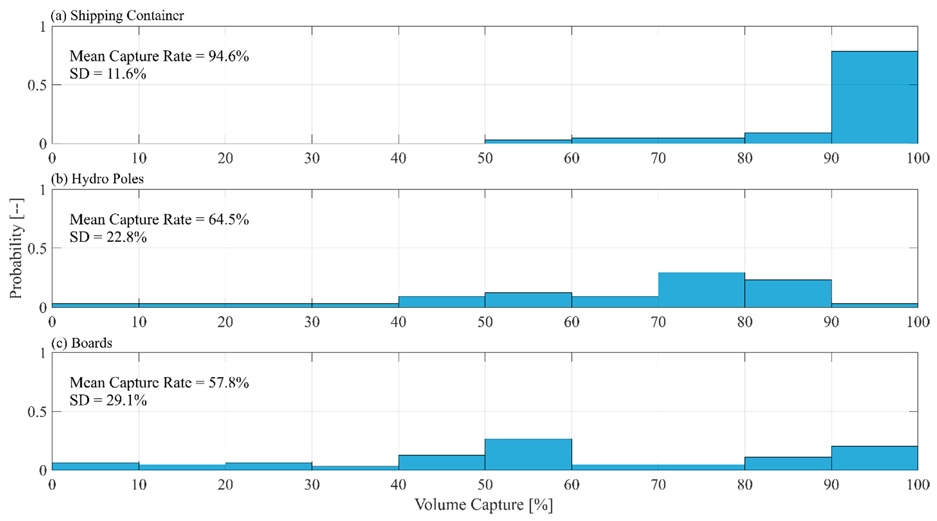
• The capture efficiency of the debris was dependent on the physical dimensions (length, width, and height) of the debris relative to the opening width of the obstacle. The larger characteristic length of the debris, the more readily the debris were captured at the obstacle.
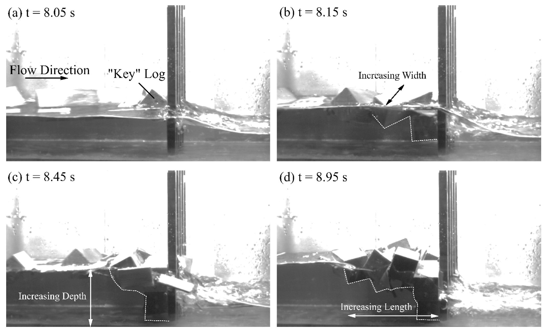
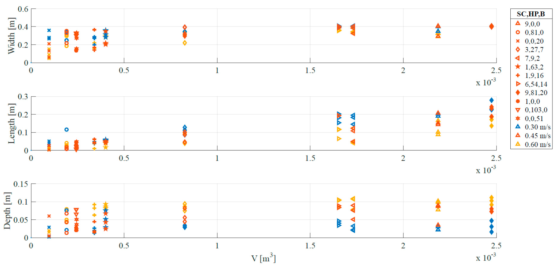
• An increase in the supplied volume of debris to the obstacle resulted in an increase in the length, width, and depth of the debris dam.
• Flow velocity had a significant influence on the blockage of the channel. The increased velocity resulted in the debris being pushed towards the bed resulting in an increased depth of the dam. Decreased velocity resulted in the formation of a debris carpet at the free-surface in front of the obstacle.
• Hydrodynamic conditions (initial flow depth and velocity) had a significant influence on the backwater levels. An increase in the Froude number resulted in a larger blockage ratio and a more pronounced backwater rise.
• Hydrodynamic conditions did not have a significant influence on the drag forces acting on the obstacle. The increase in the water depth due to the backwater rise and decrease in flow velocity resulted in no significant increase. However, the restriction of the flow around the obstacle as a result of the two-dimensional (2-D) characteristics of the flow contributed to this result and should therefore be addressed in a 3-D setting.

This study is a preliminary investigation into the mechanics of debris dam formation in flooding events. Post-tsunami field surveys of affected communities demonstrated that debris damming is a major concern in coastal flooding events. As the debris dam can influence key design criteria, such as overtopping height, flow velocities, and scour depths, careful consideration is needed in the design of infrastructure prone to such hazard. Assessing the dam formation potential and its dimensions is needed to determine design loads for tsunami resistant infrastructure. As in this experimental program the hydrodynamic forcing condition was steady-state, these results can also be applied across the wider discipline of hydraulic engineering, particularly related to design of infrastructure in debris-laden creeks and rivers.

References

- Crosset, K.M. Population Trends Along the Coastal United States: 1980–2008; Government Printing Office: Washington, DC, USA, 2005.
- Small, C.; Nicholls, R.J. A global analysis of human settlement in coastal zones. J. Coast. Res. 2003, 19, 584–599. [Google Scholar]
- Mousavi, M.E.; Irish, J.L.; Frey, A.E.; Olivera, F.; Edge, B.L. Global warming and hurricanes: The potential impact of hurricane intensification and sea level rise on coastal flooding. Clim. Chang. 2011, 104, 575–597. [Google Scholar] [CrossRef]
- Cutter, S.L.; Emrich, C.T. Moral hazard, social catastrophe: The changing face of vulnerability along the hurricane coasts. Ann. Am. Acad. Political Soc. Sci. 2006, 604, 102–112. [Google Scholar] [CrossRef]
- Ghobarah, A.; Saatcioglu, M.; Nistor, I. The impact of the 26 December 2004 earthquake and tsunami on structures and infrastructure. Eng. Struct. 2006, 28, 312–326. [Google Scholar] [CrossRef]
- Robertson, I.; Riggs, H.R.; Yim, S.C.; Young, Y.L. Lessons from Hurricane Katrina storm surge on bridges and buildings. J. Waterw. Port Coast. Ocean Eng. 2007, 133, 463–483. [Google Scholar] [CrossRef]
- Naito, C.; Cercone, C.; Riggs, H.R.; Cox, D. Procedure for site assessment of the potential for tsunami debris impact. J. Waterw. Port Coast. Ocean Eng. 2014, 140, 223–232. [Google Scholar] [CrossRef]
- Yeh, H.; Sato, S.; Tajima, Y. The 11 March 2011 East Japan earthquake and tsunami: Tsunami effects on coastal infrastructure and buildings. Pure Appl. Geophys. 2013, 170, 1019–1031. [Google Scholar] [CrossRef]
- Saatcioglu, M.; Ghobarah, A.; Nistor, I. Effects of the December 26, 2004 Sumatra earthquake and tsunami on physical infrastructure. ISET J. Earthq. Technol. 2005, 42, 79–94. [Google Scholar]
- Takagi, H.; Esteban, M.; Shibayama, T.; Mikami, T.; Matsumaru, R.; Nguyen, D.; Oyama, T.; Nakamura, R. Track analysis, simulation and field survey of the 2013 Typhoon Haiyan storm surge. J. Flood Risk Manag. 2014, 10, 1111. [Google Scholar] [CrossRef]
- Aghl, P.; Naito, C.; Riggs, H. Full-scale experimental study of impact demands resulting from high mass, low velocity debris. J. Struct. Eng. 2014, 140, 04014006. [Google Scholar] [CrossRef]
- Haehnel, R.B.; Daly, S.F. Maximum impact force of woody debris on floodplain structures. J. Hydraul. Eng. 2004, 130, 112–120. [Google Scholar] [CrossRef]
- Matsutomi, H. Method for estimating collision force of driftwood accompanying tsunami inundation flow. J. Dis. Res. 2009, 4, 435–440. [Google Scholar] [CrossRef]
- Nouri, Y.; Nistor, I.; Palermo, D.; Cornett, A. Experimental investigation of tsunami impact on free standing structures. Coast. Eng. J. 2010, 52, 43–70. [Google Scholar] [CrossRef]
- Shafiei, S.; Melville, B.W.; Shamseldin, A.Y.; Beskhyroun, S.; Adams, K.N. Measurements of tsunami-borne debris impact on structures using an embedded accelerometer. J. Hydraul. Res. 2016, 54, 1–15. [Google Scholar] [CrossRef]
- Nistor, I.; Goseberg, N.; Stolle, J. Tsunami-Driven Debris Motion and Loads: A Critical Review. Front. Built Environ. 2017, 3, 2. [Google Scholar] [CrossRef]
- Stolle, J.; Nistor, I.; Goseberg, N.; Mikami, T.; Shibayama, T. Entrainment and Transport Dynamics of Shipping Containers in Extreme Hydrodynamic Conditions. Coast. Eng. J. 2017, 1750011. [Google Scholar] [CrossRef]
- Haehnel, R.B.; Daly, S.F. Maximum Impact Force of Woody Debris on Floodplain Structures; USACE: Washington, DC, USA, 2002. [Google Scholar]
- Federal Emergency Management Agency (FEMA). Guidelines for Design of Structure for Vertical Evacuation from Tsunamis; FEMA: Washington, DC, USA, 2012; p. 646.
- Parola, A.C. Debris Forces on Highway Bridges; Transportation Research Board: Washington, DC, USA, 2000. [Google Scholar]
- Schmocker, L.; Hager, W.H. Probability of drift blockage at bridge decks. J. Hydraul. Eng. 2011, 137, 470–479. [Google Scholar] [CrossRef]
- Pagliara, S.; Carnacina, I. Bridge pier flow field in the presence of debris accumulation. In Proceedings of the Institution of Civil Engineers-Water Management; Thomas Telford Ltd.: London, UK, 2013; Volume 166, pp. 187–198. [Google Scholar]
- Melville, B.W.; Dongol, D. Bridge pier scour with debris accumulation. J. Hydraul. Eng. 1992, 118, 1306–1310. [Google Scholar] [CrossRef]
- Fenton, J. The effects of obstacles on surface levels and boundary resistance in open channels. In Proceedings of the 30th IAHR Congress, Thessaloniki, Greece, 24–29 August 2003; Volume 2, pp. 9–16. [Google Scholar]
- Schmocker, L.; Hager, W.H. Scale modeling of wooden debris accumulation at a debris rack. J. Hydraul. Eng. 2013, 139, 827–836. [Google Scholar] [CrossRef]
- Pagliara, S.; Carnacina, I. Temporal scour evolution at bridge piers: Effect of wood debris roughness and porosity. J. Hydraul. Res. 2010, 48, 3–13. [Google Scholar] [CrossRef]
- Stancanelli, L.; Lanzoni, S.; Foti, E. Propagation and deposition of stony debris flows at channel confluences. Water Resour. Res. 2015, 51, 5100–5116. [Google Scholar] [CrossRef]
- Pasha, G.A.; Tanaka, N. Effectiveness of Finite Length Inland Forest in Trapping Tsunami-Borne Wood Debris. J. Earthq. Tsunami 2016, 1650008. [Google Scholar] [CrossRef]
- Bocchiola, D.; Rulli, M.; Rosso, R. A flume experiment on the formation of wood jams in rivers. Water Resour. Res. 2008, 44. [Google Scholar] [CrossRef]
- Chock, G.Y. Design for tsunami loads and effects in the ASCE 7-16 standard. J. Struct. Eng. 2016, 142, 04016093. [Google Scholar] [CrossRef]
- National Building Code of Canada 2005; Canadian Commission on Building and Fire Codes: Ottawa, ON, Canada, 2005.
- Huang, N.E.; Shen, Z.; Long, S.R.; Wu, M.C.; Shih, H.H.; Zheng, Q.; Yen, N.-C.; Tung, C.C.; Liu, H.H. The empirical mode decomposition and the Hilbert spectrum for nonlinear and non-stationary time series analysis. In Proceedings of the Royal Society of London A: Mathematical, Physical and Engineering Sciences; The Royal Society: London, UK, 1998; Volume 454, pp. 903–995. [Google Scholar]
- Knorr, W.; Kutzner, F. EcoTransIT: Ecological Transport Information Tool—Environmental Method and Data; IFEU: Heidelberg, Germany, 2008. [Google Scholar]
- Nistor, I.; Palermo, D. Post-Tsunami Engineering Forensics: Tsunami Impact on Infrastructure. Lessons from 2004 Indian Ocean, 2010 Chile, and 2011 Tohoku Japan Tsunami Field Surveys; Esteban, M., Takagi, H., Shibayama, T., Eds.; Elsevier: Amsterdam, The Netherlands, 2015; pp. 418–434. [Google Scholar]
- Bazant, Z.P. Scaling of Structural Strength; Butterworth-Heinemann: Oxford, UK, 2005. [Google Scholar]
- McDonald, J.H. Handbook of Biological Statistics; Sparky House Publishing: Baltimore, MD, USA, 2009; Volume 2. [Google Scholar]
- Madsen, P.A.; Fuhrman, D.R.; Schaeffer, H.A. On the solitary wave paradigm for tsunamis. J. Geophys. Res. Oceans 2008, 113. [Google Scholar] [CrossRef]
- Mitobe, Y.; Adityawan, M.B.; Roh, M.; Tanaka, H.; Otsushi, K.; Kurosawa, T. Experimental Study on Embankment Reinforcement by Steel Sheet Pile Structure Against Tsunami Overflow. Coast. Eng. J. 2016, 58, 1640018. [Google Scholar] [CrossRef]
- Fritz, H.M.; Borrero, J.C.; Synolakis, C.E.; Yoo, J. 2004 Indian Ocean tsunami flow velocity measurements from survivor videos. Geophys. Res. Lett. 2006, 33. [Google Scholar] [CrossRef]
- Hughes, S.A. Physical Models and Laboratory Techniques in Coastal Engineering; World Scientific: Singapore, 1993; Volume 7. [Google Scholar]
- Bricker, J.D.; Gibson, S.; Takagi, H.; Imamura, F. On the need for larger Manning’s roughness coefficients in depth-integrated tsunami inundation models. Coast. Eng. J. 2015, 57, 1550005. [Google Scholar] [CrossRef]
- Rueben, M.; Cox, D.; Holman, R.; Shin, S.; Stanley, J. Optical Measurements of Tsunami Inundation and Debris Movement in a Large-Scale Wave Basin. J. Waterw. Port Coast. Ocean Eng. 2014, 141, 04014029. [Google Scholar] [CrossRef]
- El-Alfy, K. Backwater rise due to flow constriction by bridge piers. Thirteen. Int. Water Technol. Converence 2009, 13, 1295–1313. [Google Scholar]
- CSA. Canadian Highway Bridge Design Code; CSA: Santa Cruz, CA, USA, 2006. [Google Scholar]
- AASHTO. Bridge Design Specifications; AASHTO: Washington, DC, USA, 2012. [Google Scholar]
- Yunus, A.C.; Cimbala, J.M. Fluid mechanics fundamentals and applications. McGraw-Hill Publ. 2006, 2, 136–138. [Google Scholar]
- Anthoine, J.; Olivari, D.; Portugaels, D. Wind-tunnel blockage effect on drag coefficient of circular cylinders. Wind Struct. 2009, 12, 541–551. [Google Scholar] [CrossRef]
- Granville, P.S. Elements of the Drag of Underwater Bodies; DTIC Document; DTIC: Fort Belvoir, VA, USA, 1976. [Google Scholar]
- Stevens, B.L.; Lewis, F.L.; Johnson, E.N. Aircraft Control and Simulation: Dynamics, Controls Design, and Autonomous Systems; John Wiley & Sons: Hoboken, NJ, USA, 2015. [Google Scholar]