Estimation of Nitrate Trends in the Groundwater of the Zagreb Aquifer

1
Faculty of Mining, Geology and Petroleum Engineering, University of Zagreb, 10000 Zagreb, Croatia
2
Intellomics Ltd., 10000 Zagreb, Croatia
*
Author to whom correspondence should be addressed.
†
Deceased in February 2018.
Geosciences 2018, 8(5), 159; https://doi.org/10.3390/geosciences8050159
Submission received: 27 March 2018
/
Revised: 27 April 2018
/
Accepted: 28 April 2018
/
Published: 2 May 2018
(This article belongs to the Special Issue Groundwater Pollution)
Abstract
:Nitrates present one of the main groundwater contaminants in the world and in the Zagreb aquifer. The Zagreb aquifer presents the main source of potable water for the inhabitants of the City of Zagreb and it is protected by the Republic of Croatia. The determination of contaminants trends presents one of the main tools in groundwater body status and risk assessment. In this paper, the use of regression analysis on the aggregated data, together with confidence and prediction intervals, at different observational scales has been evaluated. Nitrate concentrations are generally decreasing in almost all areas, observed at different observational scales. It has been shown that linear regression can be efficiently used in the estimation of nitrates trends. Results showed that the calculation of confidence and prediction intervals can provide more useful conclusions than the calculation of the trend’s statistical significance. Also, the results suggest that confidence and prediction intervals can be used in groundwater body chemical status and risk assessment, respectively. Data smoothing and data aggregation are generally desirable, but have certain limitations. If too much data is aggregated, trend estimation by regression analysis can point to false conclusions. Evaluation of trends at different observational scales can provide more realistic trend estimation, as well as more precise identification of areas where groundwater protection measures should be implemented.
1. Introduction
Nitrate presents one of the main water contaminants in the world [1,2,3,4]. High nitrate concentrations have been observed in the groundwater of the Zagreb aquifer [5,6,7]. The Zagreb aquifer presents the only source of potable water for the citizens of the City of Zagreb and part of Zagreb County. It is designated as part of country’s strategic water reserves. Trends of nitrate concentrations have previously been determined for the purpose of defining the chemical status of groundwater bodies [8], in line with the requirements of the EU Water Framework Directive (WFD) [9] and Groundwater Directive (GWD) [10]. Trends should be calculated for a body or for a group of bodies, where appropriate. Generally, according to WFD and GWD provisions, trend assessment of chemical parameters should be conducted for: identification of groundwater body being at risk of failing to meet objectives under Art. 4 based on the surveillance monitoring data; and status assessment procedure and/or identification of risk of failing to meet objectives under Art. 4 based on the operational monitoring data. Previous research has shown that nitrates present one of the main groups of contaminants in the Zagreb aquifer [5]. Furthermore, two areas with elevated nitrate concentrations have been observed, while lower concentrations generally appear in the vicinity of the Sava River and in the eastern part of the aquifer [6,7].
Trends can be estimated by numerous methods. The nonparametric Mann–Kendall test [11,12] is probably the most often used method in trend estimation of water quality and hydroclimatic time series [13,14,15,16,17,18,19]. The Mann–Kendall test should be preferred to parametric trend tests when using multiple datasets because it does not require a priori assumptions related to underlying distributions [20] and it does not specify whether a trend is linear or non-linear [21]. Linear regression, piecewise regression, and logistic regression are also used in trend estimation of chemical parameters [22,23,24]. Evaluations of nitrate concentration trends on a national level have shown that groundwater recharge age determination can be very useful in trend estimation, which can correlate changes in land use and management practices with changes in groundwater quality. Also, it has been suggested that outliers and monitoring points with unstable redox conditions should be excluded from trend analysis, i.e., that only data from stable oxic environment should be used [25,26]. Additionally, entropy theory and the Hurst exponent were used to identify trends and persistence of nitrate concentrations at different spatial scales. Results suggest that nitrate concentrations in groundwater can show a scale phenomenon in both time and space, where nitrate trends show long-term persistence at intermediate and coarse scale. On the other hand, at fine scale, especially in the areas where stream–aquifer interaction is more evident, fluctuations in nitrate trends are more characteristic [27]. Furthermore, it has been established that the definition of stream–aquifer interaction can be crucial for predicting hot spots of nitrogen that were microbially driven or flow related. Also, dynamic redox conditions in the riparian zone, related to intermittent groundwater flow reversal due to surface–aquifer interaction, can produce nitrogen hot spots [28]. It is evident that various statistical constraints and geochemical features can influence trend estimation of chemical parameters, in this case nitrates. Estimation of trends by linear regression is very simple, but sometimes not appropriate. In general, water quality variables usually do not have normal distribution which suggests that non-parametric trend tests should be used. On the other hand, it is essential to define what the purpose of trend assessment is, and whether the used method is suitable for making proper and realistic conclusions. If that is achieved, the usage of simple, robust methods can be justified.
This article assesses whether linear regression, with or without data smoothing, and corresponding confidence and prediction intervals, is suitable for the estimation of nitrate concentration trend at different observational scales. It was essential to determine whether it can be effectively used in the implementation of groundwater protection measures and identification of areas vulnerable to nitrate contamination.
2. Research Area
The Zagreb aquifer is located in the northwest part of Croatia, covering approximately 350 km2 (Figure 1). It presents the only source of potable water for the citizens of the City of Zagreb and partially Zagreb County. It is designated as part of the country’s strategic water reserves.
The aquifer and its broader region are characterized by great variability in land use, pedology, lithology, and hydraulic properties. The Zagreb aquifer is made of Quaternary sediments deposited during the Middle and Upper Pleistocene and Holocene. Pleistocene deposits are lacustrine-marshy, while Holocene belong to alluvial deposits [29,30]. Hydrogeologically, the Zagreb aquifer consists of overburden, shallow, and deep aquifer layers.
The thickness of the unsaturated zone, generally disintegrated by anthropogenic influence, varies from 2 to 8 m [31]. The upper part of the unsaturated zone made of Fluvisol in the area of the Zagreb aquifer is generally permeable, except in dry periods [32], which allows the transport of contaminants to the groundwater. Nitrate concentrations are higher in the upper part of the unsaturated zone, while concentrations generally decrease with depth [33]. This is consistent with lower nitrate concentrations observed in the groundwater of Zagreb aquifer [6,7].
Shallower Holocene aquifer varies in thickness from five to 40 m, while deeper aquifer extends up to 60 m [34]. Total aquifer thickness is up to 100 m. Aquifer layers are hydraulically connected, while geochemical stratification is recognized along the depth [35]. Holocene part is in direct contact with the Sava River, which is more pronounced in the river vicinity [36]. Regional groundwater flow direction is W/NW to E/SE, while local groundwater flow strongly depends on hydrologic conditions and the Sava River fluctuations. Groundwater levels also depend on the infiltration from precipitation and leaking from sewage and water supply network, as well as due to natural boundary conditions. Inflow from the western border (contact with Samobor-Zaprešić aquifer) and the southern border has been observed [37]. Six major well fields are used for water supply (Mala Mlaka, Velika Gorica, Zapruđe, Petruševec, Sašnjak, and Žitnjak; Figure 2).
Due to the expansion of the City of Zagreb and nearby rural areas, anthropogenic influence on groundwater quality has been observed, while nitrates have been recognized as one of the main contaminants [5]. Two main areas with elevated nitrate concentrations have been identified, one on the left bank of the Sava River, in a predominantly urban area, and the other on the right bank of the Sava River, in a predominantly agricultural area. Lower nitrate concentrations are generally found in the vicinity of the Sava River and in the eastern part of the aquifer which is associated with the Sava River influence, i.e., its hyporheic zone, and aquifer deepening. It has been observed that nitrate concentrations measured in the observation wells located in the hyporheic zone are very similar to those measured at three stations in the Sava River (Jankomir, Petruševec, and Rugvica), and are generally lower than 10 mg/L of NO3−. It has been shown that aerobic conditions prevail in the Zagreb aquifer and that nitrate concentrations are more related to dissolved oxygen concentrations than redox conditions [6]. With regard to natural conditions that prevail in the Zagreb aquifer, it can be assumed that nitrification presents a more important geochemical process than denitrification, especially in the alluvial part of the aquifer. Due to regional groundwater flow and major sources of nitrate contamination, it can be assumed that in the left bank of the Sava River, nitrate concentrations are generally associated with urban pollution sources (leaking from sewage system), while in the right bank, a combination of agricultural (application of fertilizer and manure) and urban inputs (leaking from the sewage system and septic tanks) is present [6,7].
3. Materials and Methods
Groundwater quality monitoring of the Zagreb aquifer was established in 1991. In this paper, nitrate concentrations from 1991 to 2015 have been used, mainly from the National Monitoring Programme of Croatian Waters and from the monitoring programme of landfill Jakuševec. Data originate from 153 observation wells (Figure 2), a total of 13,658 nitrate concentration analysis (all nitrate data is presented as NO3−).
All the available data and analyses have been taken into account. The first insight into the data structure pointed out a few challenges. Firstly, the spatial distribution of the observation wells in the monitoring network is not ideal. They are generally located in the inflow areas of major well fields. Secondly, groundwater sampling interval is different, ranging from monthly to yearly, with no regular pattern for many observation wells. Also, some observation wells are very old, while some of them were included and/or excluded from the monitoring network on a regular basis, which resulted in the time series with different time intervals. Temporal data aggregation is a partial solution for this problem. Data aggregation has been suggested within WFD for the implementation of different tests in groundwater body chemical status assessment. It has been decided that quaternary data aggregation will be used because semi-annual or annual aggregation would generate loss of seasonality, while monthly aggregation would generate time series with a lack of data from many observation wells. In that sense, January, February, and March represent the first quarter, April, May, and June the second quarter etc. Thirdly, data regarding limit of quantification (LOQ) and limit of detection (LOD) values was incomplete, while some nitrate concentrations were not measured and were written as “0”. However, since only 237 data points were recorded as “0” or as below LOQ/LOD values, it has been decided that these data will not be used in the estimation of nitrate trends because they represent less than 2% of the total number of analysis. Most of the observation wells (about 95%) had less than five values reported as “0” or LOQ/LOD value in the whole time series. Although LOQ/LOD values can be used in form of the real measured value (for example the use of LOQ/LOD value as a number), in this case, any use of statistical analysis for the determination of outliers and extreme values would condition their exclusion from further analysis. The reason is that nitrate concentrations are much higher than the LOQ/LOD values of modern methods and instruments used for their determination, especially in areas where anthropogenic influence is evident. Also, when using large data sets obtained from different laboratories, concentrations have to be measured with analytical methods that do not generate significant differences in measured concentrations.
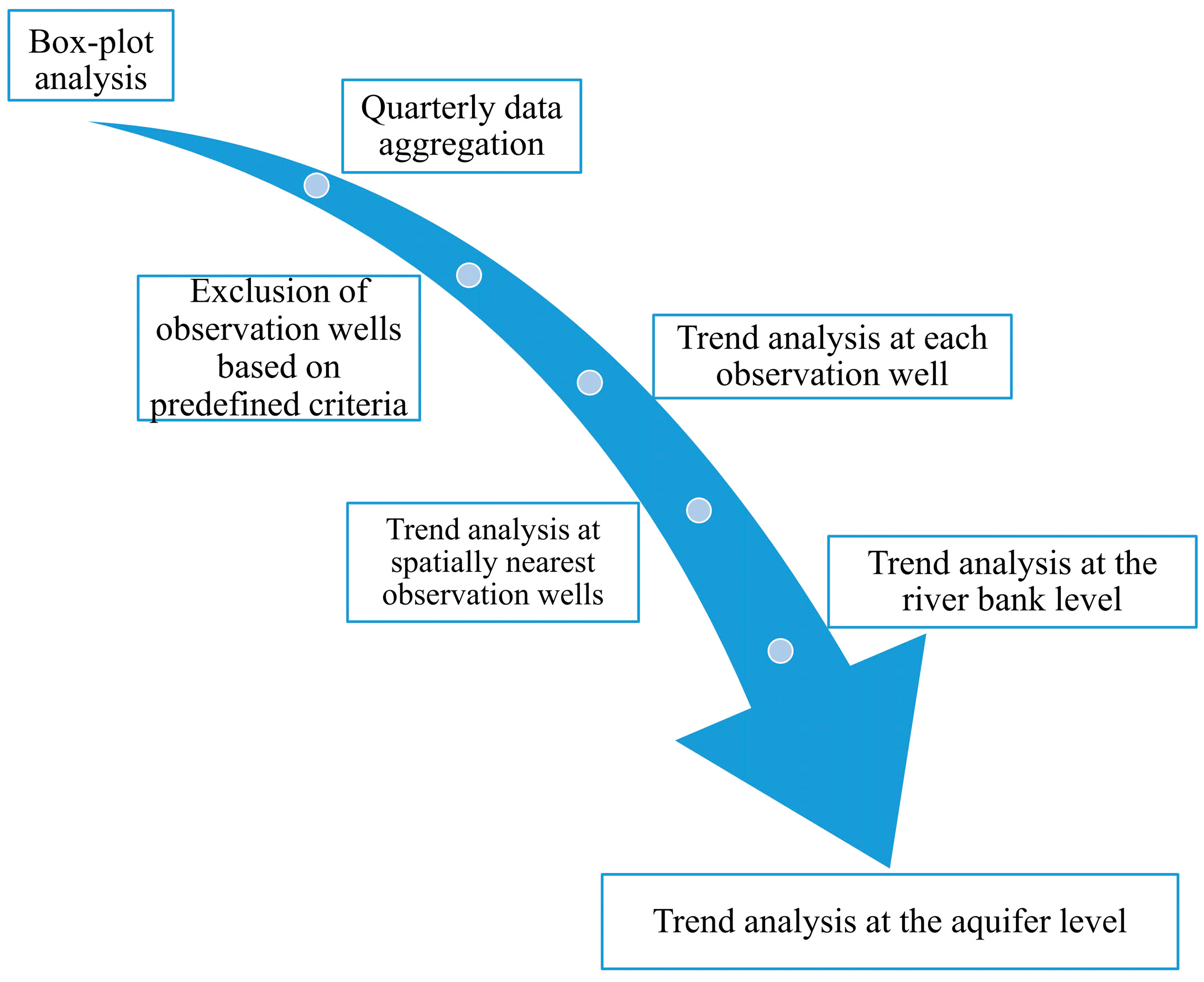
Trend analysis was conducted in seven steps (Figure 3). In the first step, box-plot analysis of NO3− concentrations was conducted at every observation well and all extreme values and outliers, a total of 427 analysis, were excluded from the analysis. Thus, the dataset was cleaned from incorrectly entered and/or incorrectly measured concentrations. Interquartile range (IQR) is defined as the difference between third quartile (Q3) and first quartile (Q1). Using standard Tukey box-plot, data points which are below Q1 − 1.5IQR or above Q3 + 1.5IQR, were considered as outliers and extremes. Most of the observation wells had less than five outliers and extreme values (Figure 4). Bin was calculated using the Scott equation [38] based on the number of samples and standard deviation.
In the second step, data from each observation well was quarterly aggregated using arithmetic mean of NO3− concentrations. During data aggregation it has been observed that a lot of quarterly data is missing.
To overcome this problem (third step), criteria for the exclusion of observation wells from trend analysis were developed. The first criterion is associated with the total number of data written in the form of LOQ/LOD or “0” values. All observation wells that had more than 30% of LOQ/LOD or “0” values in the whole available data series were excluded from the analysis. The other three criteria were related to quarterly data: (1) all observation wells used in trend analysis need to have continuous data sequence, at least 16 successive quarterly intervals; (2) observation wells should not have many gaps in the entire time series, i.e., quarterly data can be missing in no more than two successive intervals; (3) every observation well must have at least 70% of the quarterly data in the entire time interval that is selected. If all raw and aggregated quarterly data have not satisfied all of the four adopted criteria, they were excluded from the trend analysis. This resulted in the exclusion of 52 observation wells (denoted as yellow dots in Figure 2).
In the fourth step, trend analysis was conducted for each observation well separately. Simple linear regression was used, while a t-test was used for the estimation of trend’s statistical significance (α = 0.05). Trend analysis was done on aggregated quarterly data and on smoothed quarterly data, whereas LOESS nonparametric regression [39] was used for data smoothing, with smoother span of 0.3. Consequently, the possible impact of seasonality and random data on trend estimation has been reduced. Additionally, the impact of smoothing on trend analysis could be explored. Also, it was decided that trend estimation needs to be verified. In order to do so, 95% confidence and prediction intervals were used. An interval which contains mean values of y for every x, with 95% confidence, is called the 95% confidence interval for the regression line, or sometimes a 95% confidence band. On the other hand, an interval which contains the true value of y for some x, with 95% probability, is called the prediction interval. Trend analysis was conducted with two different time series. The trend line, confidence, and prediction intervals were firstly calculated on the data that did not include data from the last year. Then, the trend line as well as the confidence and prediction intervals, have been extended to the last year of time series. After that, the trend was computed together with data from the last year. Thereby, it was tested whether the new data will make a significant change in the trend, i.e., whether the newly calculated trend will exceed the estimated confidence intervals, and whether the new quarterly data will exceed the estimated prediction intervals.
After trend analysis was done for each observation well, three additional trend calculations were established, primarily associated with spatial data aggregation. In the fifth step, trend analysis was conducted for each group of observation wells (Figure 2), mostly from the well field’s inflow areas.
In the sixth step, trend analysis was separately conducted on the observation wells located on the left and the right Sava River bank, while in the seventh step, trend analysis was performed for the whole aquifer. Therefore, the results and generated conclusions could be compared at four different levels, i.e., observational scales of trend estimation.
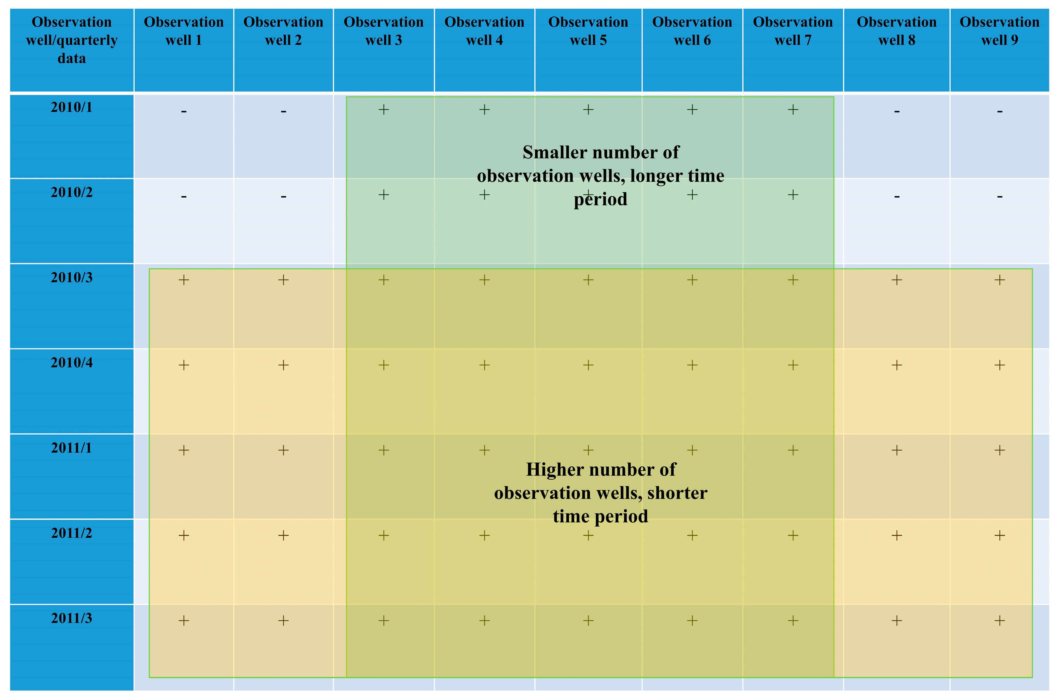
Spatial data aggregation was performed by taking the choice between using more observation wells or greater time series (Figure 5). When using more observation wells, better estimation of arithmetic mean and smaller length of overlapping time series are expected. There is no rule of thumb in deciding what the better option is, but usually minimizing the loss of data should be the main goal. An example of trend estimation for the whole Zagreb aquifer is shown in Figure 6 (with data smoothing) and Figure 7 (without data smoothing).
Box-plot analysis was performed in Dell’s Statistica 64 (version 13.1, TIBCO Software Inc., Palo Alto, CA, USA), while trend analysis (LINEST function), together with data aggregation, confidence, and prediction intervals, and calculation of statistical significance was conducted in Microsoft© Excel. All maps were made in ArcMap 10.1 (Environmental Systems Research Institute, Inc., Redlands, CA, USA), while georeferenced orthophoto images were obtained from the geoportal of the Croatian Geodetic Administration [40]. All maps are presented in the official coordinate system of the Republic of Croatia (HTRS96/TM).
4. Results and Discussion
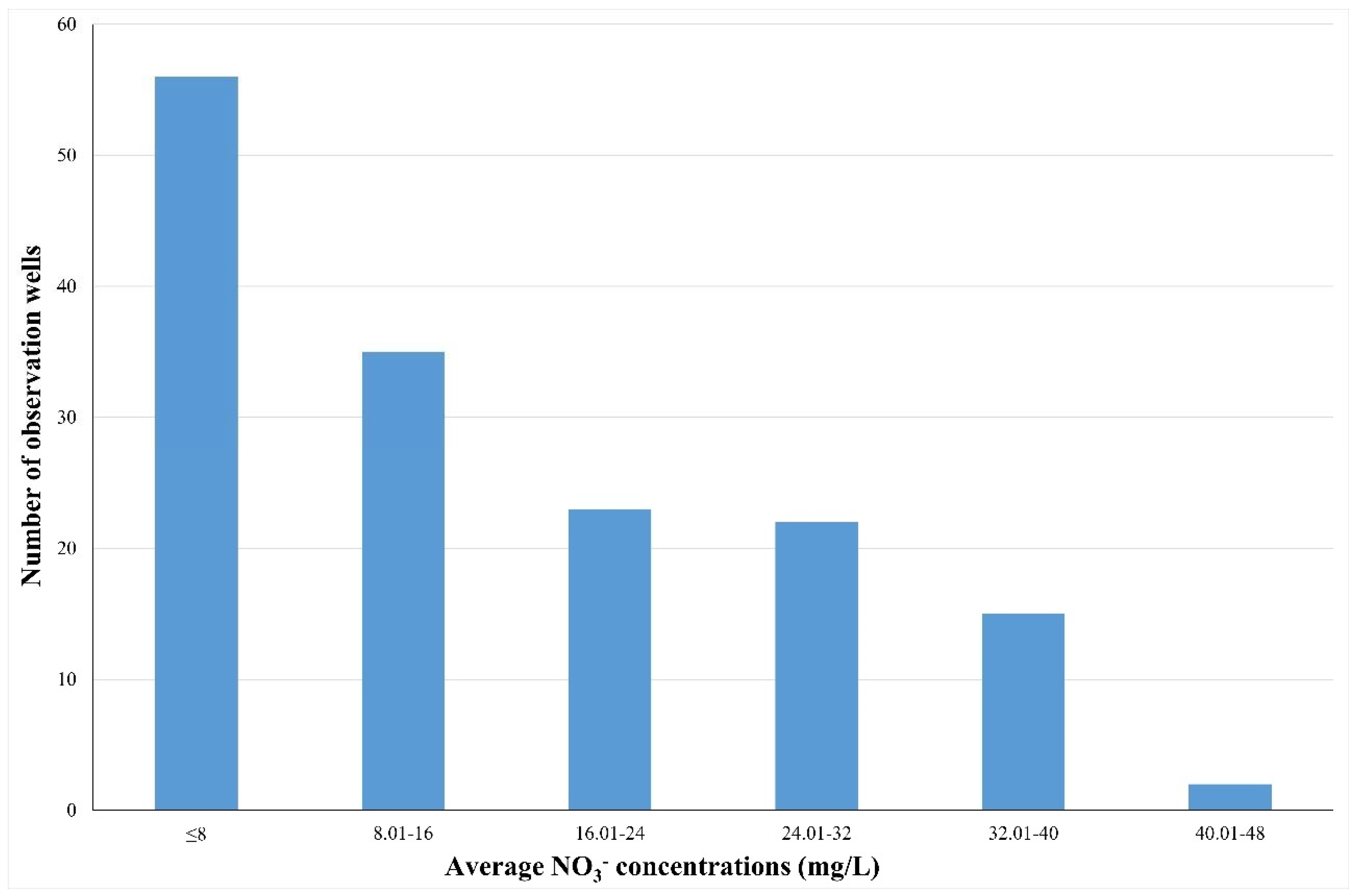
Average nitrate concentrations are lower than 16 mg/L of NO3− in 91 observation wells (Figure 8). Most of these observation wells are located in the hyporheic zone of the Sava River and have similar concentrations as those measured in the Sava River. The highest average nitrate concentration is about 44 mg/L of NO3− and is located in the urban part of the City of Zagreb, while average nitrate concentrations higher than 32 mg/L of NO3− are observed in 17 observation wells.
Summarized results of trend analysis for each observation well are shown in Table 1. Trend 1 presents a trend estimated without the last year of analysis, while Trend 2 presents a trend estimated from data that includes the last year. In Table 1, it can be seen that last year’s data did not make any significant change to the trend estimation. However, data smoothing resulted in about 30% more statistically significant trends in both cases. It seems that a small reduction of the effect of seasonality can have a large influence on trend’s statistical significance. It can be seen that data smoothing generally results in narrower confidence and prediction intervals. This results in a higher percentage of trend lines out of estimated confidence intervals, and quarterly data out of estimated prediction intervals. When evaluating results without data smoothing it can be seen that for 98 out of 101 observation wells, the trend line is within the estimated confidence intervals, while at 87 observation wells, last year’s data did not exceed the estimated prediction intervals. Even though more realistic results were expected without data smoothing (due to higher variability of raw data and, consequently, wider confidence/prediction intervals), such a good estimation of nitrate concentration trends by simple linear regression was not expected. Prediction was made for four quarters (the last available year) because it is believed that an excessively long estimation period of groundwater quality parameters in anthropogenically influenced area, with such a simple model as linear regression, is not realistic. From that point of view, trend change should be observed, i.e., updated, at least on a yearly basis. Monitoring trend changes can enable timely and effective implementation of groundwater protection measures in the most vulnerable areas.
In Table 2 (smoothed data) and Table 3 (not smoothed data), the results of nitrate concentration trend analysis at different observational scales are shown. Trends were calculated for the spatially nearest observation wells which generally coincide with well field inflow areas, after which they were calculated for the observation wells from the two Sava River banks, and in the end for the whole Zagreb aquifer. In general, almost all results suggest that there is no significant difference in results between trends generated from smoothed and not smoothed data. However, it is obvious that, when trends exist, data smoothing generates much lower p-values and more statistically significant trends. This is expected because the noise in the data is smaller, so the curve is more similar to the line, i.e., the model is more reliable in its assessment. When evaluating trends with smoothed data, it can be seen that the only difference is recorded in the area of well field Zapruđe where new data, in the last available year, caused a change from the absence of a statistically significant trend to a descending trend. This suggests that in some cases, data smoothing can be a better indicator of a change that is not so significant or is not visible when the data is not smoothed. Data without smoothing resulted in almost no difference between Trend 1 and Trend 2. The only difference can be seen in the estimation of the trend based on the data aggregated from the observation wells located on the left bank of the Sava River, where new data caused a change of descending trend to no trend. The reason is seen in the appearance of statistically significant ascending trends in the area of well fields Petruševec, Sašnjak, and Žitnjak, all of which are located on the left bank of the Sava River. All results suggested that nitrate concentrations decrease over time in almost all areas, and this coincides with previous results [6,7]. In those areas where nitrate concentrations are increasing over time, concentrations are still much lower than 50 mg/L of NO3−, which is the maximum permissible concentration according to the Drinking Water Directive [41]. If nitrate concentrations from previous studies [6,7] and calculated trends are evaluated together with regional groundwater flow and possible nitrate contamination sources, it can be seen that nitrate concentrations are higher and more persistent on the left bank of the Sava River, where urban contamination sources prevail. On the other hand, trends in all areas on the right bank of the Sava River are generally decreasing, which suggests that the application of manure and fertilizer, due to prevalence of agricultural areas, is decreasing. Also, regarding dominant geochemical processes, results suggest that nitrification is more important than denitrification, which is consistent with previous results where it was established that aerobic conditions prevail in the Zagreb aquifer, and the fact that urban pollution sources introduce nitrogen in a large extent in the form of ammonium ion, which is then transformed into nitrates.
When evaluating trend lines that exceed estimated confidence intervals, and data that exceeds estimated prediction intervals in the spatially aggregated data, the results point to different conclusions. Even though data without smoothing generated trend lines within estimated confidence intervals, evaluation of last year’s data and estimated prediction intervals showed a lot more deviations. When evaluating smoothed data, in 50% of cases the data appeared outside of the estimated prediction intervals, while 33% of last year’s data is noticed outside of predicted intervals when using not smoothed data. The exception is seen for the whole aquifer, where results suggest that last year’s data did not have that much influence on trend estimation and data prediction. The very likely explanation is that high and low nitrate concentrations measured in the last year are spatially well balanced and deviations from general trend cannot be seen when all data are aggregated together. That is consistent with the fact that there are two major areas with elevated nitrate concentrations [6,7], one located on the left, and the other located on the right bank of the Sava River.
Trend analysis conducted in seven steps (Figure 3) showed that used methodology can be very efficient in trend estimation because it resolves a few very important issues. Most of the bad data, as well as not good enough observation wells, were excluded from the analysis, which has partially been recognized in previous research [25]. Spatial aggregation made it possible to generate conclusions at different observational scales, which is also consistent with some previous research that showed differences in trends when they were evaluated at fine, intermediate, and coarse scales [27]. When using long data series, which contain a large number of data, spatial and temporal data aggregation may lead to bias. In this case, all results suggest that data aggregation could be useful in the estimation of nitrate concentration trends. However, if too many observation wells are included, i.e., the evaluated area is too large, there may be a problem in identifying vulnerable areas. Also, the use of different observational scales of trend estimation, regardless of the data smoothing, provided more efficient trend estimation and the identification of the areas in which it is necessary to carry out protection measures. It must be emphasized that within this trend analysis, the impact of biogeochemical processes which take place in the unsaturated zone were not evaluated due to the lack of data. They could potentially have great influence on nitrate concentrations and consequently trend estimation, especially in the hyporheic zone of the Sava River. Dynamic stream–aquifer interaction and constant fluctuation of groundwater levels very often change the direction of groundwater flow and transport of the contaminants. Besides that, depth to groundwater is changing which may have an effect on changing the aerobic/anaerobic conditions, especially in extreme hydrological conditions, which are very important for the stability of different nitrogen species. Accordingly, future research should be focused on defining the influence of the unsaturated zone on nitrate concentrations, as well as on defining the importance of processes, i.e., nitrification and denitrification, that have impact on nitrate concentrations in the saturated zone.
Confidence intervals can be more useful than the calculation of trend statistical significance because they show boundaries in which a trend line can move. If between those boundaries a trend cannot change its sign, generally it can be assumed that it is significant. Also, confidence intervals projected based on trends calculated on the spatially aggregated data, in almost all cases, especially with smoothed data, showed that data from the last year of measurement does not influence trend direction. That means they can be used as markers of significant trend’s change at one-year intervals. Also, if they suggest the existence of an ascending trend and the occurrence of predicted confidence intervals above the given threshold value, they can be used as a reliable tool for groundwater chemical status assessment. On the other hand, prediction intervals can be used as markers for the determination of groundwater body chemical risk assessment. For example, if chemical concentrations and estimated trend confidence intervals are lower than the defined threshold value, but prediction interval suggests that this threshold can be exceeded in the following years, the groundwater body could be marked as being at risk of not reaching good chemical status. However, the use of prediction intervals can have numerous limitations when using too many observation wells, especially in areas where anthropogenic influence is very pronounced, as is the case with the urban part of the City of Zagreb. In that case, the use of data without smoothing would provide much more realistic predictions.
5. Conclusions
It can be seen that nitrate contamination exists in the groundwater of the Zagreb aquifer. Although the presence of various sources of nitrate contamination has been established, trend analysis has shown that nitrate concentration trends are decreasing, except in a few isolated areas. Simple linear regression can be very efficiently used in trend estimation, along with confidence and prediction intervals. However, its use becomes more limited when using too much spatially aggregated data because aquifer chemistry, as well as anthropogenic influence, can change over time and space. Confidence and prediction intervals can be very useful in the estimation of groundwater body chemical status and risk assessment. It has been shown that data smoothing provides more statistically significant trends when trends exist and more strict intervals, providing a faster method of identifying slower trend change. Data aggregation in groundwater chemistry research is desirable and necessary at the level of each observation well. Spatial aggregation can also be very useful. However, spatial aggregation, especially in areas where there is a large difference in groundwater chemistry and anthropogenic influence, must be conducted very carefully, so that the analysis does not lead to false conclusions. Within this trend analysis, the influence of geochemical processes which take place in the unsaturated zone was not evaluated. In order to reduce uncertainty in the trend estimation, future research should be focused on the definition of biogeochemical processes that have an impact on nitrate concentrations, as well as on a more detailed definition of spatial and temporal changes in aerobic and anaerobic conditions in the Zagreb aquifer. Evaluation of trends at different observational scales is a very efficient tool for trend assessment, and it can provide more realistic and more detailed identification of vulnerable areas.
Author Contributions
Z.K. has collected data. Z.K., D.Š. and D.S. have analyzed the data. All authors participated in designing the methodology for trend estimation. Z.K. made trend calculations. Z.K. and Z.N. wrote most of the manuscript, while D.Š., D.S., and A.B. have provided substantial edits and reviews of drafts of this manuscript.
Acknowledgments
The authors would like to thank Croatian Waters for the data obtained within the project “Definition of trends and groundwater status assessment in the Pannonian part of the Croatia”, and Zagreb holding d.o.o., for providing data of groundwater monitoring in the area of landfill Jakuševec. Publication process is supported by the Development Fund of the Faculty of Mining, Geology and Petroleum Engineering, University of Zagreb.
Conflicts of Interest
The authors declare no conflict of interest.
References
- Almasri, M.N. Nitrate contamination of groundwater: A conceptual management framework. Environ. Impact Assess. Rev. 2007, 27, 220–242. [Google Scholar] [CrossRef]
- Xue, D.; Botte, J.; De Baets, B.; Accoe, F.; Nestler, A.; Taylor, P.; Van Cleemput, O.; Berglund, M.; Boeckx, P. Present limitations and future prospects of stable isotope methods for nitrate source identification in surface- and groundwater. Water Res. 2009, 43, 1159–1170. [Google Scholar] [CrossRef] [PubMed]
- Xu, S.; Kang, P.; Sun, Y. A stable isotope approach and its application for identifying nitrate source and transformation process in water. Environ. Sci. Pollut. Res. 2016, 23, 1133–1148. [Google Scholar] [CrossRef] [PubMed]
- Pennino, M.J.; Compton, E.J.; Leibowitz, S.G. Trends in Drinking Water Nitrate Violations across the United States. Environ. Sci. Technol. 2017, 51, 13450–13460. [Google Scholar] [CrossRef] [PubMed]
- Nakić, Z.; Ružičić, S.; Posavec, K.; Mileusnić, M.; Parlov, J.; Bačani, A.; Durn, G. Conceptual model for groundwater status and risk assessment—Case study of the Zagreb aquifer system. Geol. Croat. 2013, 66, 55–76. [Google Scholar] [CrossRef]
- Kovač, Z.; Nakić, Z.; Pavlić, K. Influence of groundwater quality indicators on nitrate concentrations in the Zagreb aquifer system. Geol. Croat. 2017, 70, 93–103. [Google Scholar] [CrossRef]
- Kovač, Z.; Cvetković, M.; Parlov, J. Gaussian simulation of nitrate concentration distribution in the Zagreb aquifer. J. Maps 2017, 13, 727–732. [Google Scholar] [CrossRef]
- Nakić, Z.; Bačani, A.; Parlov, J.; Duić, Ž.; Perković, D.; Kovač, Z.; Tumara, D.; Mijatović, I.; Špoljarić, D.; Ugrina, I.; et al. Definiranje Trendova i Ocjena Stanja Podzemnih voda na Području Panonskog Dijela Hrvatske (Definition of Trends and Groundwater Status Assessment in the Pannonian Part of the Croatia). Available online: http://www.voda.hr/sites/default/files/dokumenti/definiranje_trendova_i_ocjena_stanja_podzemnih_voda_na_podrucju_panonskog_dijela_hrvatske_2016.pdf (accessed on 20 March 2018).
- EU Water Framework Directive (2000/60/EC). Available online: http://eur-lex.europa.eu/legal-content/EN/TXT/?uri=CELEX:32000L0060 (accessed on 20 March 2018).
- Groundwater Directive (2006/118/EC). Available online: https://eur-lex.europa.eu/legal-content/EN/TXT/?uri=CELEX%3A32006L0118 (accessed on 20 March 2018).
- Mann, H.B. Nonparametric tests against trend. Econometrica 1945, 13, 245–259. [Google Scholar] [CrossRef]
- Kendall, M.G. Rank Correlation Methods; Charles Griffin: London, UK, 1975. [Google Scholar]
- Morán-Tejeda, E.; Lorenzo-Lacruz, J.; López-Moreno, J.I.; Rahman, K.; Beniston, M. Streamflow timing of mountain rivers in Spain: Recent changes and future projections. J. Hydrol. 2014, 517, 1114–1127. [Google Scholar] [CrossRef]
- Mekonnen, A.D.; Woldeamlak, B. Variability and trends in rainfall amount and extreme event indices in the Omo-Ghibe River Basin, Ethiopia. Reg. Environ. Chang. 2014, 14, 799–810. [Google Scholar] [CrossRef]
- Tabari, H.; Meron, T.T.; Willems, P. Statistical assessment of precipitation trends in the upper Blue Nile River basin. Stoch. Environ. Res. Risk Assess. 2015, 29, 1751–1761. [Google Scholar] [CrossRef]
- Gebremedhin, K.; Shetty, A.; Nandagiri, L. Analysis of variability and trends in rainfall over Northern Ethiopia. Arab. J. Geosci. 2016, 9. [Google Scholar] [CrossRef]
- Lutz, S.R.; Mallucci, S.; Diamantini, E.; Majone, B.; Bellin, A.; Merz, R. Hydroclimatic and water quality trends across three Mediterranean river basins. Sci. Total Environ. 2016, 571, 1392–1406. [Google Scholar] [CrossRef] [PubMed]
- Pavlić, K.; Kovač, Z.; Jurlina, T. Trend analysis of mean and high flows in response to climate warming—Evidence from karstic catchments in Croatia. Geofizika 2017, 34, 157–174. [Google Scholar] [CrossRef]
- Diamantini, E.; Lutz, S.R.; Mallucci, S.; Majone, B.; Merz, R.; Bellin, A. Driver detection of water quality trends in three large European river basins. Sci. Total Environ. 2018, 612, 49–62. [Google Scholar] [CrossRef] [PubMed]
- Hirsch, R.M.; Slack, J.R. A nonparametric trend test for seasonal data with serial dependence. Water Resour. Res. 1984, 20, 727–732. [Google Scholar] [CrossRef]
- Yue, S.; Pilon, P.; Cavadias, G. Power of the Mann-Kendall test and the Spearman’s rho test for detecting monotonic trends in hydrological time series. J. Hydrol. 2002, 259, 254–271. [Google Scholar] [CrossRef]
- Grath, J.; Scheidleder, A.; Uhlig, S.; Weber, K.; Kralik, M.; Keimel, T.; Gruber, D. The EU Water Framework Directive: Statistical Aspects of the Identification of Groundwater Pollution Trends, and Aggregation of Monitoring Results; Final Report; European Commission: Brussels, Belgium, 2001; Available online: https://circabc.europa.eu/sd/a/a1f194ce-8684-436c-a130-ec88ee781bd2/Groundwater%20trend%20report.pdf (accessed on 20 March 2018).
- Vargas-Yáñez, M.; Zunino, P.; Benali, A.; Delpy, M.; Pastre, F.; Moya, F.; García-Martínez, M.C.; Tel, E. How much is the Western Mediterranean really warming and salting? J. Geophys. Res. 2010, 115. [Google Scholar] [CrossRef]
- Nolan, B.; Hitt, K.; Ruddy, B. Probability of Nitrate Contamination of Recently Recharged Groundwaters in the Conterminous United States. Environ. Sci. Techol. 2002, 36, 2138–2145. [Google Scholar] [CrossRef]
- Hansen, B.; Thorling, L.; Dalgaard, T.; Erlandsen, M. Trend Reversal of Nitrate in Danish Groundwater—A Reflection of Agricultural Practices and Nitrogen Surpluses since 1950. Environ. Sci. Techol. 2011, 45, 228–234. [Google Scholar] [CrossRef] [PubMed]
- Hansen, B.; Thorling, L.; Schullehner, J.; Termansen, M.; Dalgaard, T. Groundwater nitrate response to sustainable nitrogen management. Nature 2017, 7, 8566. [Google Scholar] [CrossRef] [PubMed]
- Dwivedi, D.; Mohanty, B.P. Hot Spots and Persistence of Nitrate in Aquifers across Scales. Entropy 2016, 18, 25. [Google Scholar] [CrossRef]
- Dwivedi, D.; Arora, B.; Steefel, C.I.; Dafflon, B.; Versteeg, R. Hot spots and hot moments of nitrogen in a riparian corridor. Water Resour. Res. 2018, 54, 205–222. [Google Scholar] [CrossRef]
- Velić, J.; Durn, G. Alternating Lacustrine-Marsh Sedimentation and Subaerial Exposure Phases during Quaternary: Prečko, Zagreb, Croatia. Geol. Croat. 1993, 46, 71–90. [Google Scholar]
- Velić, J.; Saftić, B.; Malvić, T. Lithologic Composition and Stratigraphy of Quaternary Sediments in the Area of the “Jakuševec” Waste Depository (Zagreb, Northern Croatia). Geol. Croat. 1999, 52, 119–130. [Google Scholar]
- Ružičić, S.; Mileusnić, M.; Posavec, K. Building Conceptual and Mathematical Model for Water Flow and Solute Transport in the Unsaturated zone at Kosnica Site. Min. Geol. Pet. Eng. Bull. 2012, 25, 21–31. [Google Scholar]
- Ružičić, S.; Kovač, Z.; Nakić, Z.; Kireta, D. Fluvisol permeability estimation using soil water content variability. Geofizika 2017, 34, 141–155. [Google Scholar] [CrossRef]
- Ružičić, S.; Kovač, Z.; Tumara, D. Physical and chemical properties in relation to soil permeability in the area of the Velika Gorica well field. Min. Geol. Pet. Eng. Bull. 2018, 33, 73–81. [Google Scholar] [CrossRef]
- Nakić, Z.; Posavec, K.; Parlov, J.; Bačani, A. Development of the Conceptual Model of the Zagreb Aquifer System. In The Geology in Digital Age: Proceedings of the 17th Meeting of the Association of European Geological Societies Belgrade, Serbia, 14–16 September 2011; MAEGS 17/Banjac, Nenad (ur.); Serbian Geological Society: Belgrade, Serbia, 2011; pp. 169–174. ISBN 978-86-86053-10-7. [Google Scholar]
- Marković, T.; Brkić, Ž.; Larva, O. Using hydrochemical data and modelling to enhance the knowledge of groundwater flow and quality in an alluvial aquifer of Zagreb, Croatia. Sci. Total Environ. 2013, 458–460, 508–516. [Google Scholar] [CrossRef] [PubMed]
- Posavec, K.; Vukojević, P.; Ratkaj, M.; Bedeniković, T. Cross-correlation Modelling of Surface Water—Groundwater Interaction Using the Excel Spreadsheet Application. Min. Geol. Pet. Eng. Bull. 2017, 32, 25–32. [Google Scholar] [CrossRef]
- Posavec, K. Identifikacija i Prognoza Minimalnih Razina Podzemne Vode Zagrebačkoga Aluvijalnog Vodonosnika Modelima Recesijskih Krivulja (Identification and Prediction of Minimum Groundwater Levels of Zagreb Alluvial Aquifer Using Recession Curve Models). Ph.D. Thesis, Faculty of Mining, Geology and Petroleum Engineering, University of Zagreb, Zagreb, Croatia, 2006. (In Croatian). [Google Scholar]
- Scott, D.W. On Optimal and Data-Based Histograms. Biometrika 1979, 66, 605–610. [Google Scholar] [CrossRef]
- Cleveland, W.S. Robust Locally Weighted Regression and Smoothing Scatterplots. J. Am. Stat. Assoc. 1979, 74, 829–836. [Google Scholar] [CrossRef]
- Croatian Geodetic Administration. Available online: http://geoportal.dgu.hr/podaci-i-servisi/svi-servisi-i-aplikacije/ (accessed on 20 March 2018).
- Drinking Water Directive (98/83/EC). Available online: https://eur-lex.europa.eu/legal-content/EN/TXT/?uri=CELEX%3A31998L0083 (accessed on 20 March 2018).
Figure 1.
Research area.
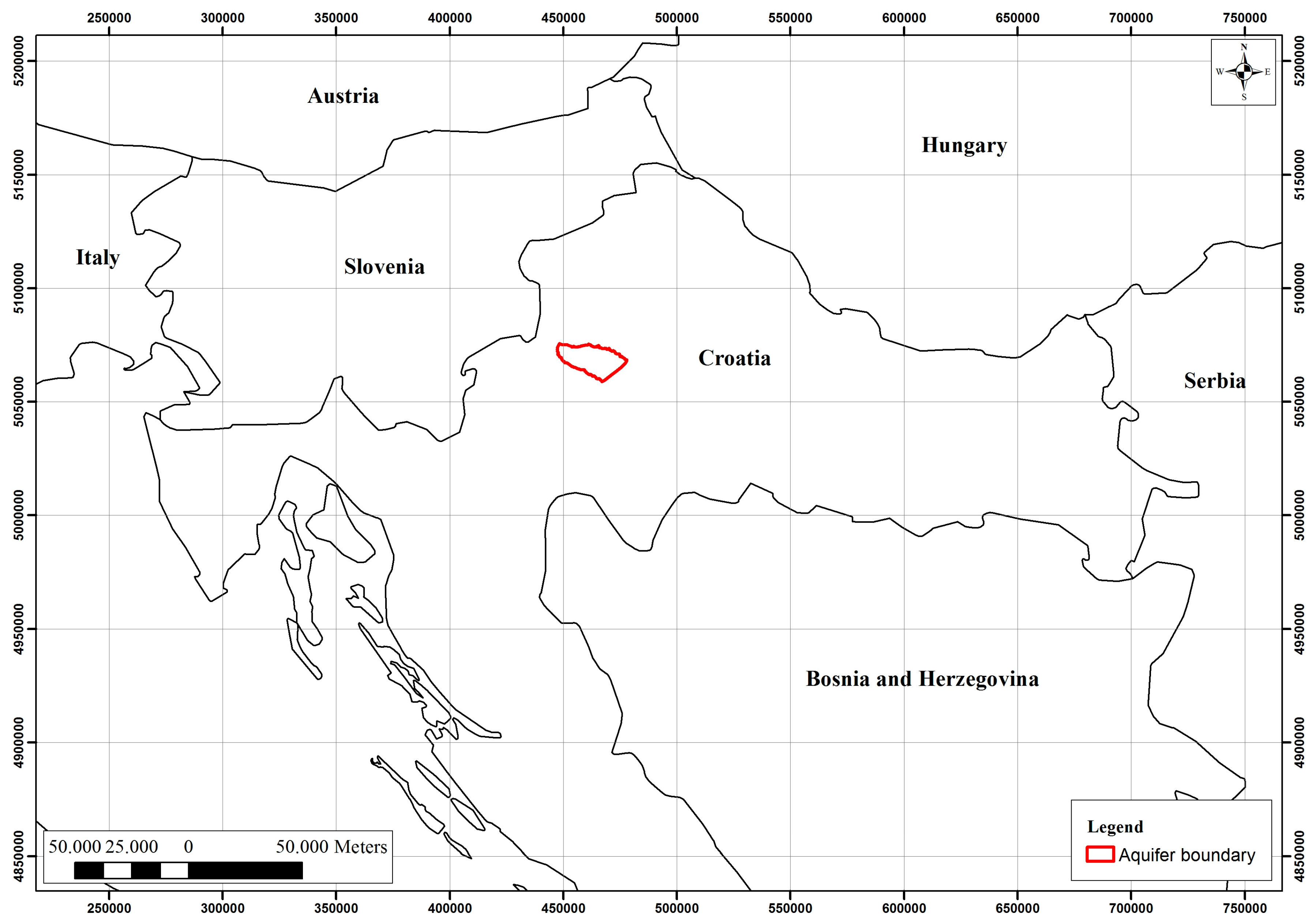
Figure 2.
Observation wells used in trend analysis.
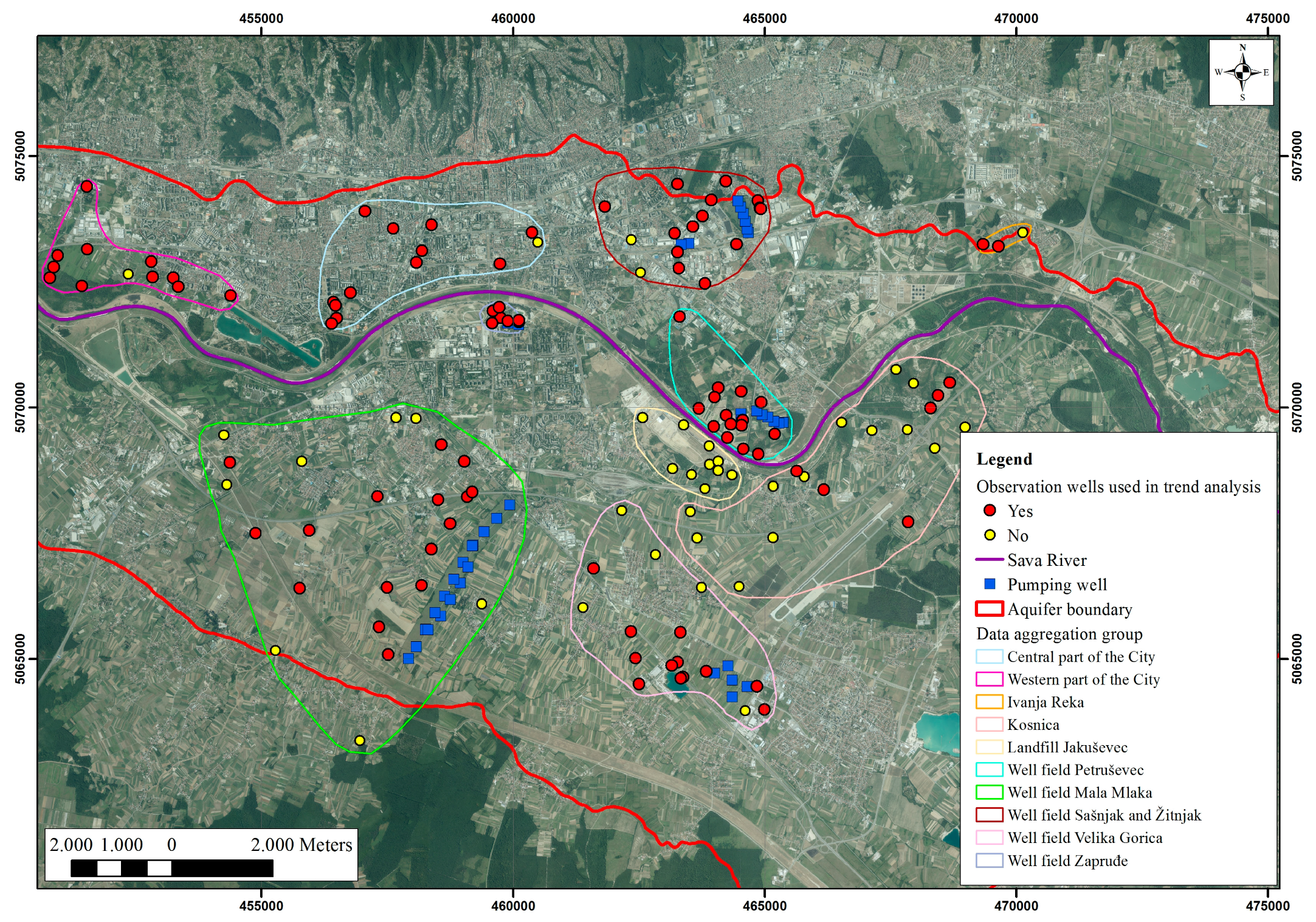
Figure 3.
Trend analysis estimation flow chart.

Figure 4.
Observed extreme values and outliers at 153 observation wells.
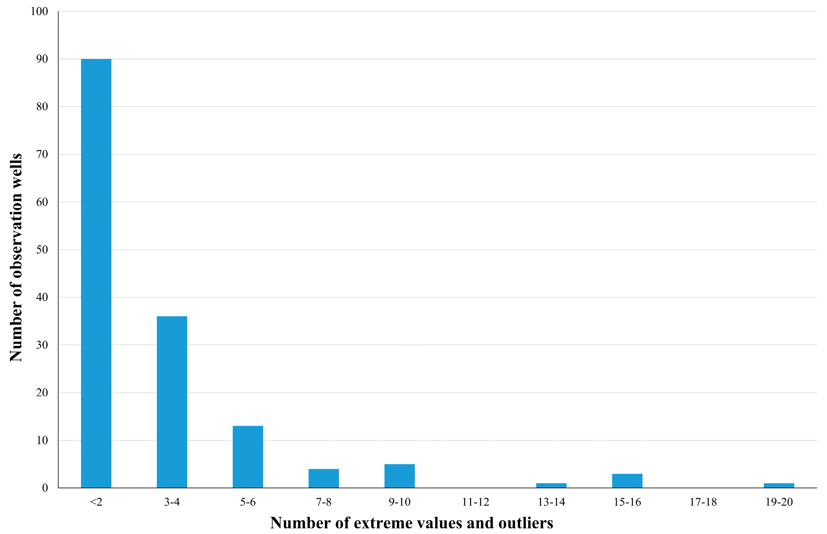
Figure 5.
Illustration of possible choices when doing spatial data aggregation.

Figure 6.
Trend estimation with data smoothing for the whole aquifer.
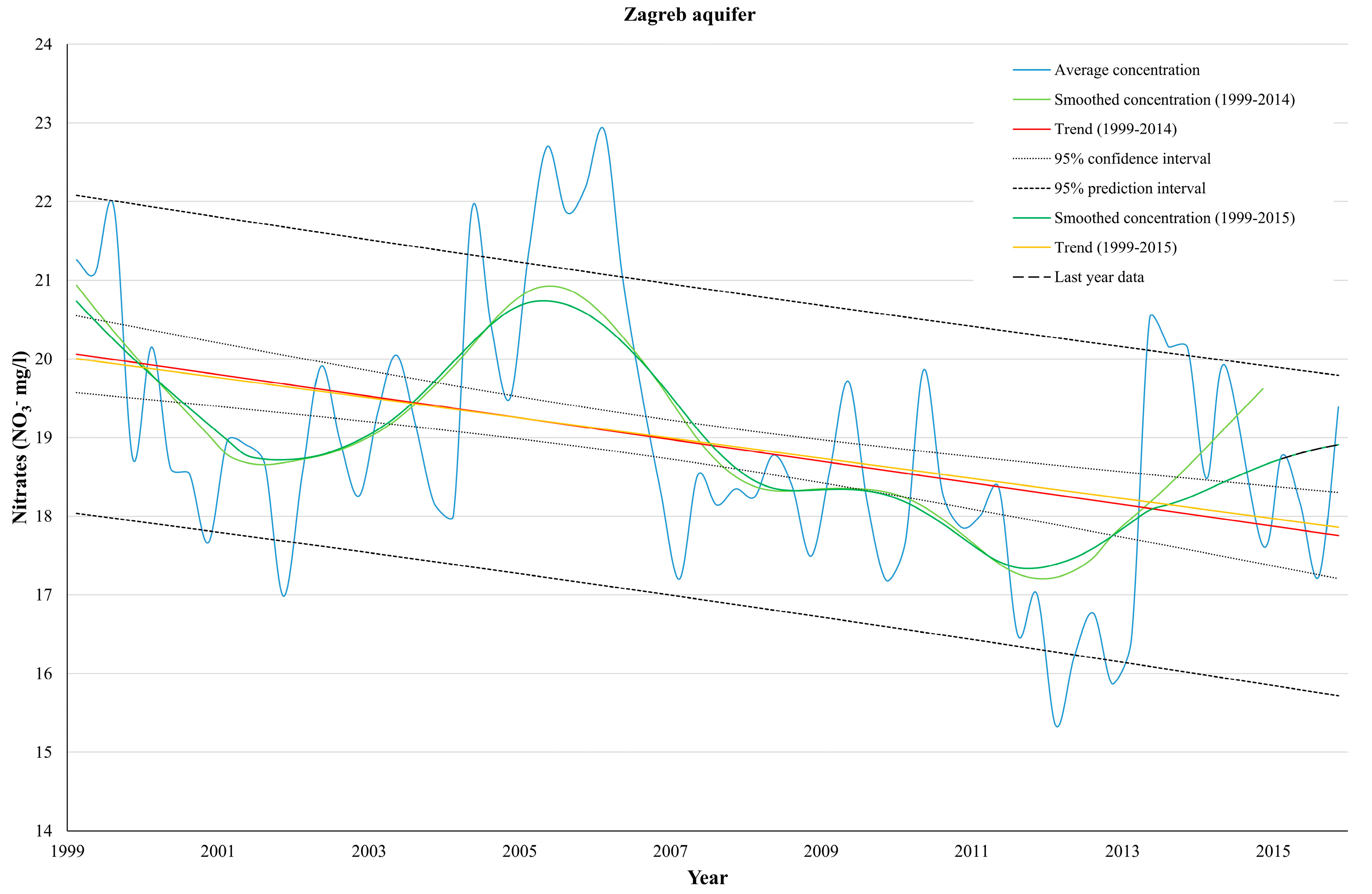
Figure 7.
Trend estimation without data smoothing for the whole aquifer.
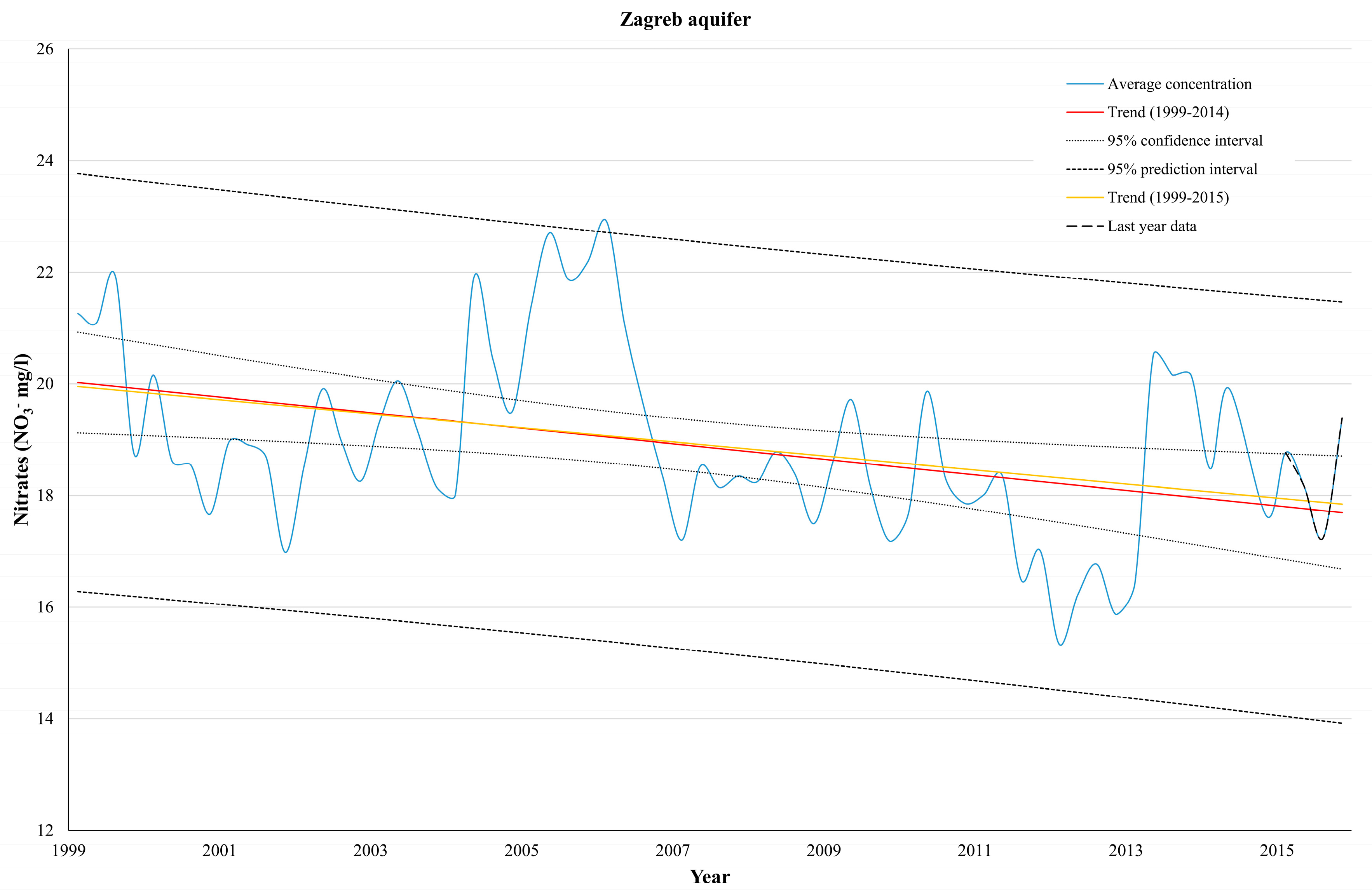
Figure 8.
Average nitrate concentrations in all observation wells from 1991 until 2015.


Table 1.
Summary results of nitrate trends estimation on the level of observation well.
| Data | Smoothed Data | Not Smoothed Data | ||||||
|---|---|---|---|---|---|---|---|---|
| Trend 1 | Trend 2 | Trend within Confidence Intervals | Data within Prediction Intervals | Trend 1 | Trend 2 | Trend within Confidence Intervals | Data within Prediction Intervals | |
| Statistically significant trend | 83 | 84 | 74/101 | 69/101 | 66 | 68 | 98/101 | 87/101 |
| Ascending trend | 52 | 49 | 44 | 43 | ||||
| Descending trend | 31 | 35 | 22 | 25 | ||||
| No trend | 18 | 17 | 35 | 33 | ||||
Table 2.
Summary results of nitrate trends estimation at different observational scales (smoothed data).
Table 2.
Summary results of nitrate trends estimation at different observational scales (smoothed data).
| Smoothed Data | ||||||||||
|---|---|---|---|---|---|---|---|---|---|---|
| Area | Trend 1 | Statistically Significant | Trend Direction | p-Value | Trend 2 | Statistically Significant | Trend Direction | p-Value | Trend within Confidence Interval | Data within Prediction Interval |
| Central part of the City | 1994–2014 | Yes | Descending | 9.10 × 10⁻³¹ | 1994–2015 | Yes | Descending | 1.73 × 10⁻³² | Yes | No |
| Western part of the City | 1994–2014 | Yes | Descending | 2.91 × 10⁻²⁵ | 1994–2015 | Yes | Descending | 1.26 × 10⁻³⁰ | Yes | Yes |
| Ivanja Reka | 1999–2012 | Yes | Descending | 6.14 × 10⁻³¹ | 1999–2013 | Yes | Descending | 2.90 × 10⁻¹⁹ | No | No |
| Well field Sašnjak and Žitnjak | 1998–2014 | Yes | Ascending | 1.28 × 10⁻⁹ | 1998–2015 | Yes | Ascending | 2.02 × 10⁻⁸ | Yes | Yes |
| Well field Petruševec | 1999–2014 | Yes | Ascending | 7.04 × 10⁻¹¹ | 1999–2015 | Yes | Ascending | 2.82 × 10⁻¹³ | Yes | No |
| Well field Mala Mlaka | 1995–2014 | Yes | Descending | 1.98 × 10⁻⁸ | 1995–2015 | Yes | Descending | 4.35 × 10⁻¹³ | Yes | Yes |
| Well field Zapruđe | 2007–2013 | No | No trend | 9.74 × 10⁻¹ | 2007–2014 | Yes | Descending | 3.88 × 10⁻² | No | No |
| Well field Velika Gorica | 2005–2014 | Yes | Descending | 6.57× 10⁻¹⁰ | 2005–2015 | Yes | Descending | 3.05 × 10⁻¹² | Yes | Yes |
| Kosnica | 2003–2012 | Yes | Descending | 9.03 × 10⁻¹⁴ | 2003–2013 | Yes | Descending | 3.72 × 10⁻¹⁴ | Yes | Yes |
| Left bank of the Sava River | 1999–2014 | Yes | Descending | 8.92 × 10⁻⁷ | 1999–2015 | Yes | Descending | 2.02 × 10⁻³ | No | No |
| Right bank of the Sava River | 2003–2014 | Yes | Descending | 6.56 × 10⁻¹² | 2003–2015 | Yes | Descending | 4.38 × 10⁻¹¹ | Yes | No |
| Zagreb aquifer | 1999–2014 | Yes | Descending | 2.32 × 10⁻⁷ | 1999–2015 | Yes | Descending | 7.65 × 10⁻⁹ | Yes | Yes |
Table 3.
Summary results of nitrate trend’s estimation at different observational scales (not smoothed data).
Table 3.
Summary results of nitrate trend’s estimation at different observational scales (not smoothed data).
| Not Smoothed Data | ||||||||||
|---|---|---|---|---|---|---|---|---|---|---|
| Area | Trend 1 | Statistically Significant | Trend Direction | p-Value | Trend 2 | Statistically Significant | Trend Direction | p-Value | Trend within Confidence Interval | Data within Prediction Interval |
| Central part of the City | 1994–2014 | Yes | Descending | 6.72 × 10⁻²⁰ | 1994–2015 | Yes | Descending | 1.54 × 10⁻²⁰ | Yes | Yes |
| Western part of the City | 1994–2014 | Yes | Descending | 8.74 × 10⁻¹² | 1994–2015 | Yes | Descending | 7.13 × 10⁻¹⁴ | Yes | Yes |
| Ivanja Reka | 1999–2012 | Yes | Descending | 3.41 × 10⁻¹¹ | 1999–2013 | Yes | Descending | 1.03 × 10⁻⁸ | Yes | No |
| Well field Sašnjak and Žitnjak | 1998–2014 | Yes | Ascending | 7.54 × 10⁻⁴ | 1998–2015 | Yes | Ascending | 1.91 × 10⁻³ | Yes | Yes |
| Well field Petruševec | 1999–2014 | Yes | Ascending | 3.10 × 10⁻³ | 1999–2015 | Yes | Ascending | 1.69 × 10⁻⁴ | Yes | Yes |
| Well field Mala Mlaka | 1995–2014 | Yes | Descending | 3.32 × 10⁻⁴ | 1995–2015 | Yes | Descending | 2.58 × 10⁻⁶ | Yes | No |
| Well field Zapruđe | 2007–2013 | No | No trend | 9.96 × 10⁻¹ | 2007–2014 | No | No trend | 5.75 × 10⁻¹ | Yes | Yes |
| Well field Velika Gorica | 2005–2014 | Yes | Descending | 2.63 × 10⁻⁴ | 2005–2015 | Yes | Descending | 1.28 × 10⁻⁴ | Yes | Yes |
| Kosnica | 2003–2012 | Yes | Descending | 7.52 × 10⁻⁴ | 2003–2013 | Yes | Descending | 6.54 × 10⁻⁴ | Yes | Yes |
| Left bank of the Sava River | 1999–2014 | Yes | Descending | 6.36 × 10⁻³ | 1999–2015 | No | No trend | 8.63 × 10⁻² | Yes | No |
| Right bank of the Sava River | 2003–2014 | Yes | Descending | 8.94 × 10⁻⁷ | 2003–2015 | Yes | Descending | 7.75 × 10⁻⁶ | Yes | No |
| Zagreb aquifer | 1999–2014 | Yes | Descending | 2.31 × 10⁻³ | 1999–2015 | Yes | Descending | 1.94 × 10⁻³ | Yes | Yes |
© 2018 by the authors. Licensee MDPI, Basel, Switzerland. This article is an open access article distributed under the terms and conditions of the Creative Commons Attribution (CC BY) license (http://creativecommons.org/licenses/by/4.0/).
Share and Cite
MDPI and ACS Style
Kovač, Z.; Nakić, Z.; Špoljarić, D.; Stanek, D.; Bačani, A. Estimation of Nitrate Trends in the Groundwater of the Zagreb Aquifer. Geosciences 2018, 8, 159. https://doi.org/10.3390/geosciences8050159
AMA Style
Kovač Z, Nakić Z, Špoljarić D, Stanek D, Bačani A. Estimation of Nitrate Trends in the Groundwater of the Zagreb Aquifer. Geosciences. 2018; 8(5):159. https://doi.org/10.3390/geosciences8050159
Chicago/Turabian StyleKovač, Zoran, Zoran Nakić, Drago Špoljarić, David Stanek, and Andrea Bačani. 2018. "Estimation of Nitrate Trends in the Groundwater of the Zagreb Aquifer" Geosciences 8, no. 5: 159. https://doi.org/10.3390/geosciences8050159
Note that from the first issue of 2016, this journal uses article numbers instead of page numbers. See further details here.