Virtual Crop Water Export Analysis: The Case of Greece at River Basin District Level


1
Department of Civil Engineering, University of Thessaly, 38334 Volos, Greece
2
Wageningen Economic Research, 2502 LS The Hague, The Netherlands
*
Author to whom correspondence should be addressed.
Geosciences 2018, 8(5), 161; https://doi.org/10.3390/geosciences8050161
Submission received: 18 March 2018
/
Revised: 16 April 2018
/
Accepted: 27 April 2018
/
Published: 3 May 2018
(This article belongs to the Special Issue Ecological Modeling in Geosciences: Ecosystem Services Assessment and Valuation)
Abstract
:An analysis of virtual crop water export through international trade is conducted for Greece, downscaled to the River Basin District (RBD) level, in order to identify critical “hotspots” of localized water shortage in the country. A computable general equilibrium model (MAGNET) was used to obtain the export shares of crops and associated irrigation water was calculated for all major crops in Greece. A distinction between virtual crop water locally consumed and traded internationally was made for all Greek RBDs. Cotton was identified as a large water consumer and virtual water exporter, while GR08 and GR10 were identified as the RBDs mostly impacted. The value of virtual water exported was calculated for all crop types and fruits and vegetables were identified as the crop most beneficial, since they consume the least water for the obtained value.
1. Introduction
Europe’s economic prosperity and well-being is intrinsically linked to its natural environment—from fertile soils to clean air and water. Natural resources enable the functioning of the economy (globally, continentally, nationally and regionally) and support our quality of life. These resources include (renewable and non-renewable) energy, food and fiber from crop production, quality of soil, and water [1]. Global demand for fresh water, for example, is foreseen to increase until 2030 by 40%, while demand for food by 35% [2]. Such trends largely depend on growth in global population, increased urbanization and changes in consumption patterns. Continuing current trends in the use of these natural resources means that nations are living beyond their biocapacity, thus creating an ecological deficit [3]. Specifically for Europe, despite the environmental improvements of recent decades, the challenges it faces today are considerable, especially in the Mediterranean, where water scarcity is increasing under the pressure of climate change and natural capital is being degraded by socioeconomic activities, such as agriculture. Beyond Europe, global pressures on the environment have grown at an unprecedented rate since the 1990s, driven not least by economic and population growth, and changing consumption patterns. Furthermore, food, water and climate are interconnected [4] and addressing food security issues under climate change automatically puts pressure on water resources. Even though there is enough freshwater on the planet to serve the needs of global population, it is unevenly distributed and too much of it is wasted, polluted and unsustainably managed [5]. This practically means that according to climate conditions and location, some countries may suffer from water scarcity while others are favored by physical water abundance. This unequal allocation of water drives a diversity in water availability for human life, ecosystems, industry and agriculture; while is fundamentally and inextricably tied to the history of politics, economics, food production, and population dynamics. Modern societies, under the threat of irreversible depletion of the available water reserves are starting to see the need to revise their overall water use practices towards an integrated and effective sustainable plan of water resource management.
At the same time, growing understanding of the characteristics of Europe’s environmental challenges and their interdependence with economic and social systems in a globalized world through trade has brought with it increasing recognition that special attention is needed to the concept of “embedded resources” in the goods being traded. “Virtual” or “embedded” water in the chain of all productive processes that goods undergo till they are marketed and exposed to international trade is a relevant approach towards water balance analysis, on a global level [6]. The virtual water concept implies the “hidden” water behind goods and essentially incorporates the volume of water that is transferred from one country to another through commerce. Virtual water analysis is considered as a lever to reveal the background water flows embedded on the trading net of commodities. Since the conception of the idea, numerous studies have been conducted in terms of quantifying virtual water flows between countries [7,8,9]. Hoekstra and Hung [10] introduced a research scientific report highlighting crop virtual water trade flows for the period 1995–1999, concluding to the share of the nations with largest net virtual water exports and imports. In another article, Zimmer and Renault [11] addressed methodological issues and provided preliminary results on global virtual trade, deducing the main contributors among crops, livestock, and fishery products. China, a country with a large fluctuation in water resource availability throughout its borders and with high inter-regional commercial activity was thoroughly investigated by Guan and Hubacek [12], who concluded that the trade structure between North and South China is not very favorable with regards to water resource allocation and efficiency.
At international level, “virtual water trade” has geopolitical effects and causes dependencies between countries. Since virtual water is economically invisible and politically silent [13], national policy makers have to dedicate on revealing the dynamics of virtual water in order to assess trade impact on water resource availability. In other words, it is beneficial for nations with scarce water resources to redesign their national imports-exports policies by importing virtual water, through the import of water-intensive products and exporting less water consuming products. In light of this, transaction of goods should follow a securing food and water availability pattern depending on the coupling of economic and environmental status of the country [10].
In this paper, an analysis of virtual crop water of Greece on a River Basin District (RBD) level is conducted. Virtual crop water demands for 2011 are calculated and mapped on the Greek RBDs on a monthly time step, thus capturing the seasonality and identifying the impact of agriculture on local water resource availability. The Modular Applied GeNeral Equilibrium modelling Tool (MAGNET) is used to estimate the future levels (up to 2050) of Greek agricultural production and exports and associated virtual crop water, which is either consumed locally or exported. The analysis reveals the crops that contribute mostly to the virtual crop water export in Greece and identifies the corresponding RBDs that are mostly impacted. The analysis is extended to include the monetary value of exported agricultural products; this value is compared against the corresponding embedded water of these products, producing useful information on the value of exported crops per virtual crop water unit.
2. Materials and Methods
There are 14 RBDs in Greece; they have been defined for districts with similar hydrogeologic conditions and they constitute the regional level water management unit nationally. The Water Framework Directive 2000/60/EC (WFD) defines the RBD as the indicative spatial unit for which the corresponding plans are drawn up; thus, virtual crop water analysis for Greece on an RBD level is deemed as most relevant to reveal the impact of agriculture on local water resource availability. Although Greece has one of the greatest water resource potentials per capita in the Mediterranean area and should theoretically have ample water for its population and traditional water uses, water is not evenly distributed in space and time. The maximum precipitation is recorded in the western parts, where the available water resources are consequently plentiful, while in other regions of the country, precipitation is much lower and available water resources are insufficient to meet the demand. Due to this inequality in water distribution, both in space and time, some regions of Greece are facing long-term water shortage problems [14]. The Greek Ministry of the Environment and Climate Change (YPEKA) reports results of its National Water Monitoring Network on groundwater quantity; according to these results (found in nmwn.ypeka.gr/map), and when it comes to water quantity, several RBDs (GR01, GR02, GR03, GR04, GR05, GR11, GR12, GR13, GR14) are classified as having adequate water quantities, two RBDs as having medium supplies (GR06, GR07), and three RBDs as being highly stressed (GR08, GR09, GR10). Figure 1 shows the distribution of these RBDs. This map has been developed with data provided by the Hellenic Ministry of the Environment and Climate Change, where the water resource quantities in river basins are classified as “good”, “bad” or “unknown”. Depending on the surface area occupied by “bad” river basins that correspond to each RBD, they are classified as “low”, “medium” or “high stress” in the map shown in Figure 1. The map attests the uneven distribution of groundwater resources availability throughout Greece, while it enhances the ascertainment that considering water resource availability on a national level may be misleading, since water scarcity is localized in specific regions. Specifically, the Thessaly and Central Macedonia plains (GR08 and GR10 respectively) are the most intensively cultivated in Greece, requiring large amounts of irrigation water, creating a water deficit that is seasonal reaching its peak during the summer months, when precipitation is at its lowest [15]. As shown in Figure 1, these RBDs are the ones with the worst groundwater quantity state (highly-stressed).
2.1. MAGNET Model
In this study we use the Modular Applied GeNeral Equilibrium modelling Tool (MAGNET) to estimate the future levels of Greek agricultural production and exports. MAGNET has been used in policy analysis and the exploration of future economic trends particularly related to agriculture. MAGNET is a recursive, dynamic, multiregional, multisector, general equilibrium model that covers the entire global economy and is fully documented in Woltjer et al. [16]. MAGNET, based on the comparative static general equilibrium model GTAP [17], is structured in a modular fashion, where additional modelling extensions can be added and removed as needed to address the question at hand. The core of the model is a set of national or aggregated national input-output tables of payments and receipts between all sectors and including the household consumption and bilateral trade flows. Production is structured using a nested constant elasticity of substitution (CES) function, where the nested inputs and substitution elasticities can be structured differently to capture sector production characteristics. Consumption is divided between private consumption, government consumption and savings using Cobb-Douglas function and private consumption further specified using a constant-difference elasticity (CDE) function among consumption goods. MAGNET can be linked to the IMAGE model [18], which provides projections for agricultural land availability, yield changes and livestock productivity.
To project sector and trade developments in Greece and the rest of the world towards 2050, MAGNET is run using exogenous GDP and population projections to endogenously calibrate the productivity increases of labor and other production inputs. The GDP and population projections are in line with the Business As usual Shared Socio-Economic Pathway (SSP2). The SSPs [19] are a set of qualitative narratives of future development. SSP2 represents the business as usual development pathway with the continuation of current trends in, for example, GDP, population, diet, energy use, land use regulation and agricultural yield efficiency increases. The specific SSP2 instantiation used in MAGNET is documented in van Meijl et al. [20]. MAGNET was used in order to calculate the future production of a series of generic crop categories for Greece up to 2050, having as a point of reference their production quantities in 2011. Each generic crop category included in the analysis is subdivided into specific crop types, as shown in Table 1, in which the crop categories and their production quantities are listed; these quantities are used as input data to the model.
MAGNET was used to produce the generic crop categories and their export shares; in Table 2, the market values in 2011 and the corresponding values for 2030 and 2050 are presented. These values use constant 2011 prices; therefore, the changes in production value are purely due to changes in the quantity of production.
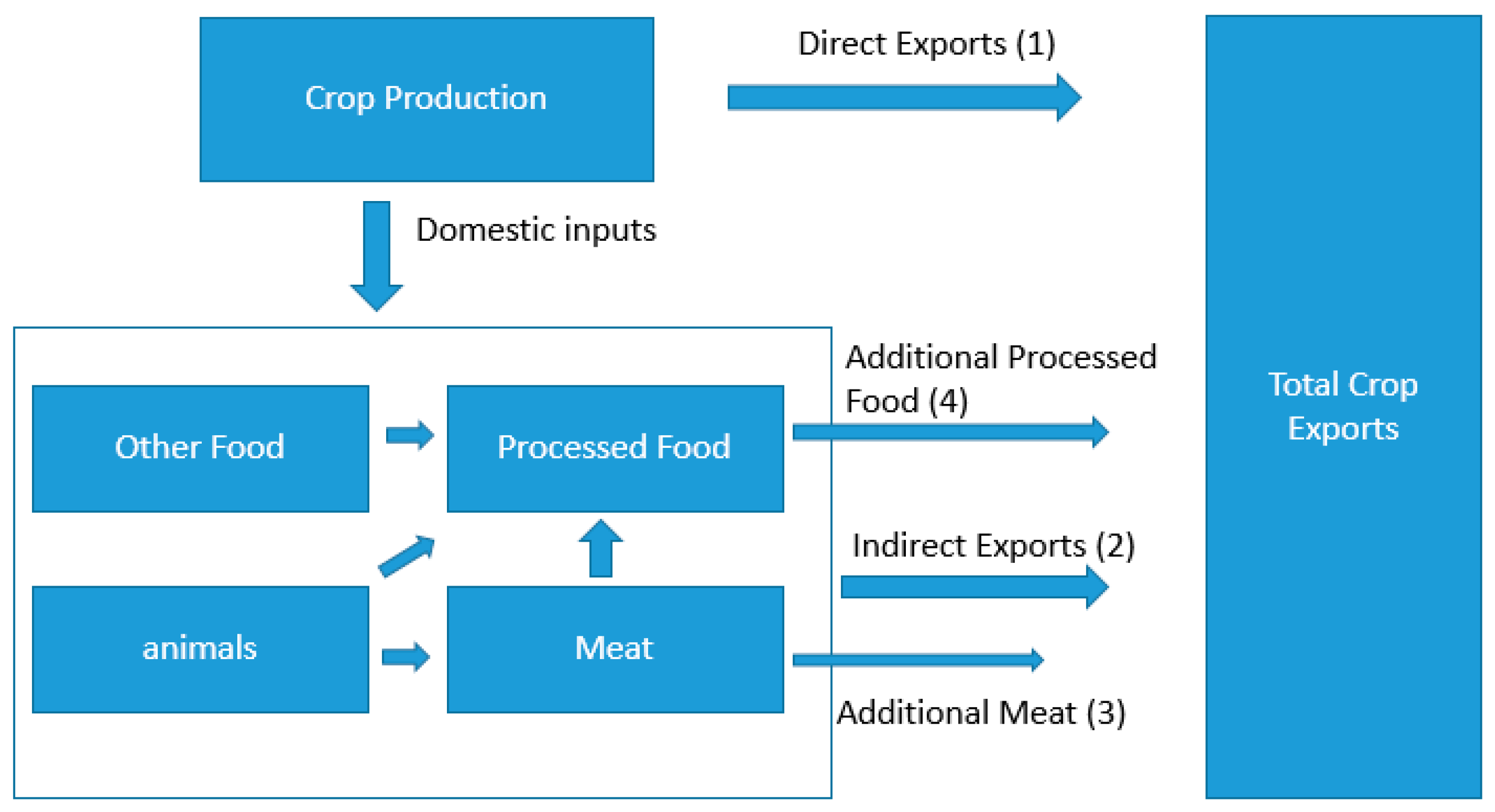
To estimate the total share of Greek crops that are created for foreign consumption we include not only the crops that are directly exported, but also include indirect crop exports, that is, crops that are first used as inputs in another sector and which are then further exported. Examples of this include paddy rice as an input into processed rice, which is then exported, or grains as input into cattle, which are then exported. This estimation is done on the basis of input shares and where necessary was also done iteratively (for example, grain into cattle which is further taken as input into cattle meat). Figure 2 is a schematic that illustrates these relationships; quantities marked in the figure as (1) through (4) are further described in the corresponding formulas. Total crop exports for each period are calculated as the sum of quantities (1) through (4).
where, is the production of sector i, valued in 2011 USD; is the unitless ratio (exports of sector i)/(production of sector i) both terms valued at 2011 USD; is the unitless ratio (inputs from sector i into sector j)/(production of sector i) both terms valued at 2011 USD.
The indexes c, di, di1, an, mt, proF sets containing respectively: crops, direct inputs of crops, direct inputs of crops less processed food and other industry, animals, meat, and processed food. A Table (Table A1) is included in the Appendix A that contains the list of MAGNET sectors in each of these sets.
Quantity (1) represents the direct exports of each crop, these were taken directly from the MAGNET model. Quantity (2) represents the portion of crops that were indirectly exported by a sector, which took the crops as a direct input, examples here would be processed rice, sugar and vegetable oil. We excluded the services sector where we assumed crops consumed by the services sector, for example restaurants, were all used domestically. Quantity (3) represents the indirect exports of crops via the exports of meat which itself consumes crops indirectly through the consummation of the “animals” sector. Quantity (4) represents the exports of crops indirectly through processed foods first via another sector. For example, the exports of oil seeds via vegetable oil via processed foods. The estimation of total crop exports including direct and indirect is given by the sum of products (1)–(4). Table 3 shows the value of the crops, calculated by MAGNET, which are destined for export either directly or indirectly through other sectors. The projections till 2050 provide information concerning the evolution of the percentage export shares per crop type.
2.2. Data on Water Demand per Crop Type
Water demand per crop type was calculated using Equation (5).
where, is water consumed for crop i, on month j and on RBD k; is the area occupied by crop i, on RBD k; is real water needs for crop i, on month j.
Agricultural areas for each crop type were obtained from the Hellenic Statistical Authority (ELSTAT) [21], where irrigated crop types, corresponding areas and production quantities are listed for all Greek regions. Since Greek regions do not exactly match RBDs, ArcGIS was used to downscale this information and transform it from regional to RBD level. Naturally, ELSTAT data matched EUROSTAT data, which is the primary source of data for MAGNET, ensuring that our base year data were in compliance with MAGNET data. This way, even though MAGNET provides production quantities for different crop categories only on a national level, it was possible to disaggregate national-level data to the 14 Greek RBDs. Monthly irrigation data per crop type was obtained by an online tool provided by the Institute for Agricultural Research of Cyprus [22], which provides monthly water needs for each crop type. It should be noted here that all calculations were done on the basis of actual crop water needs and losses and/or irrigation technologies were not taken into account. Obtained data were cross-checked with EUROSTAT annual irrigation water consumption data reported per RBD for Greece and a general agreement was established, essentially validating the approach. After obtaining data series on water demand per crop type for all irrigated crops and different RBDs in Greece on a monthly time step for 2011, MAGNET projections for agricultural production for years up to 2050 enabled the generation of similar data series for water demand for consecutive years.
Applying the export shares derived from MAGNET by 2050 to the crop production volumes in each RBD provides the basic information needed to calculate how much water is finally exported per crop type. It should be noted here that differing climatic conditions that might affect irrigated crop water demand were not taken into account; in other words, it was assumed that irrigation demand stayed the same throughout the years. This assumption is considered to be safe, based on data reported by the European Environment Agency (EEA) on how climate change affects water requirements of agricultural crops across Europe, in which projections are presented specifically for grain maize [23]. The projected annual rate of change of crop water deficit (the difference between crop water demand and rainfall) for maize during the growing season in Greece for the period 2015 to 2045 is expected to only vary between −10 and 10% for most of the country. This deficit change includes changes in rainfall, which is expected to drop for Mediterranean countries, thus increasing estimated deficit values for Greece. Since the future deficit estimated by the EEA is relatively small for Greece, it is not expected that the assumption will introduce significant error in the results presented herein. Changes in water demand presented here are a result only of changes in production for SSP2, which is calculated by MAGNET, taking into account its assumptions. Using MAGNET projections, the exported virtual crop water is calculated accordingly.
3. Results
3.1. Locally Used and Exported Virtual Crop Water
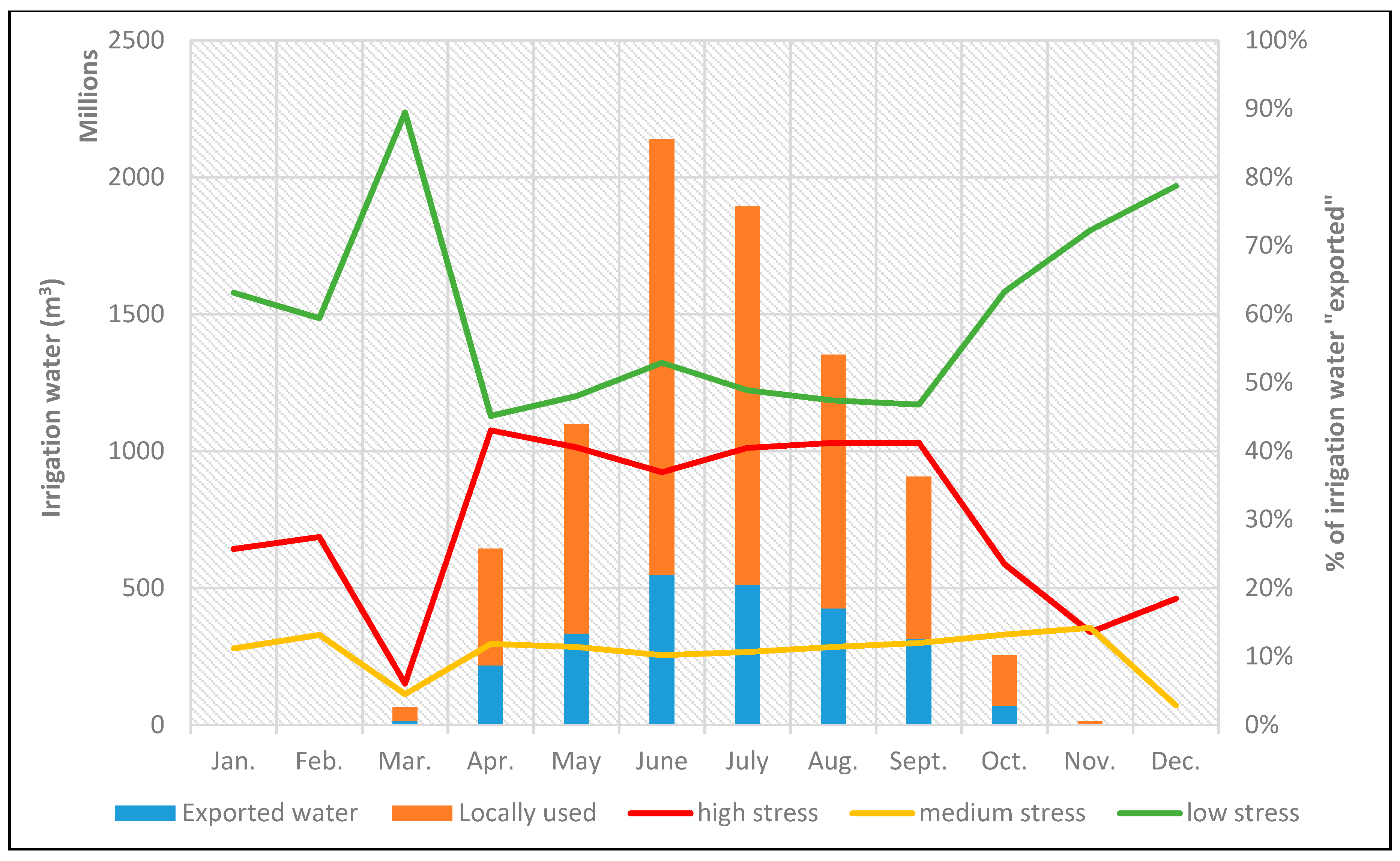
Irrigation water is calculated for all crops produced in Greece and is further divided in two categories: irrigation water for crops consumed within the Greek territory and irrigation water for crops ultimately exported through international trade. In Figure 3, this distinction between locally used and exported virtual crop water is shown for the base year 2011. Furthermore, exported water is downscaled to the RBD level, in order to distinguish which RBDs are impacted the most, following the notation used in Figure 1 for their state regarding water quantity. As expected, irrigation water demand is much higher during the summer months of June and July, intensifying the high stress various RBDs face due to agricultural activities. In terms of “exported virtual water”, the three highly stressed districts (GR08, GR09 and GR10) seem to carry the biggest load, since about 40% of exported water comes from these RBDs for six months of the year (April to September). If medium-stressed districts are added to this percentage, then approximately 50% of exported water originates from these highly impacted districts.
3.2. Water-Intensive Crops Exported per RBD
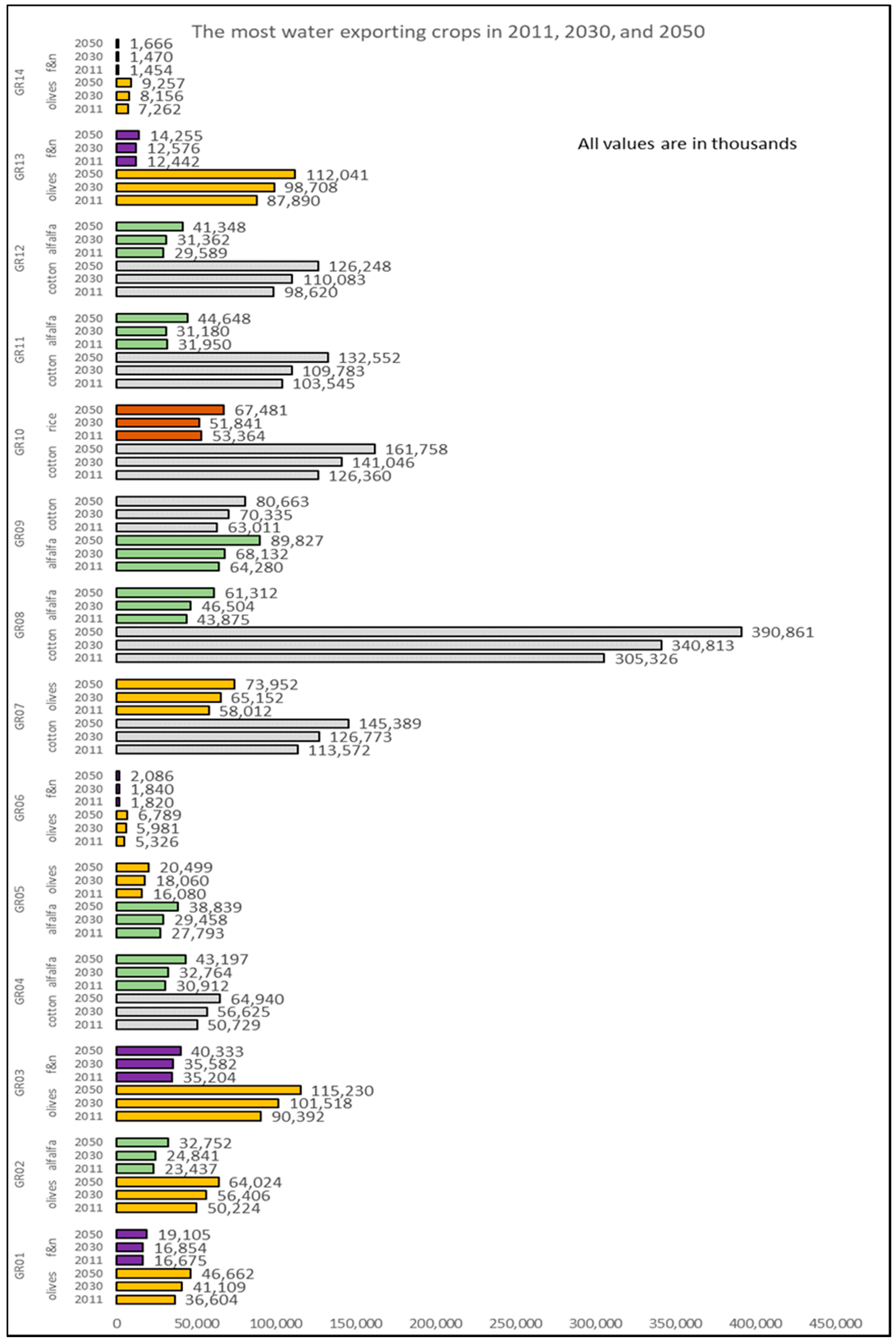
Figure 4 shows the two crop types with the highest virtual crop water exported per RBD in Greece for years 2011, 2030 and 2050. It is obvious that GR08 contributes mostly to water exports, through cotton. Indeed, cotton seems to stand out almost in all RBDs where it is cultivated, namely GR04, GR07, GR08, GR09, GR10, GR11 and GR12. Olives also seem to stand out in the RBDs of the Peloponnese (GR01, GR02 and GR03) and in Crete (GR13), but their export share in virtual crop water is second to cotton. Alfalfa, fruits & nuts (f & n), and paddy rice also appear on the list as significant virtual crop water exporters. On almost all cases, with only minor exceptions, virtual crop water exports are projected to be increasing over time, all the way to 2050, enhancing the view that agricultural production will remain a strong sector in the Greek economy and making even more urgent the need to manage water resources efficiently in the years to come.
3.3. Economic Versus Environmental Aspects of Virtual Crop Water Exported
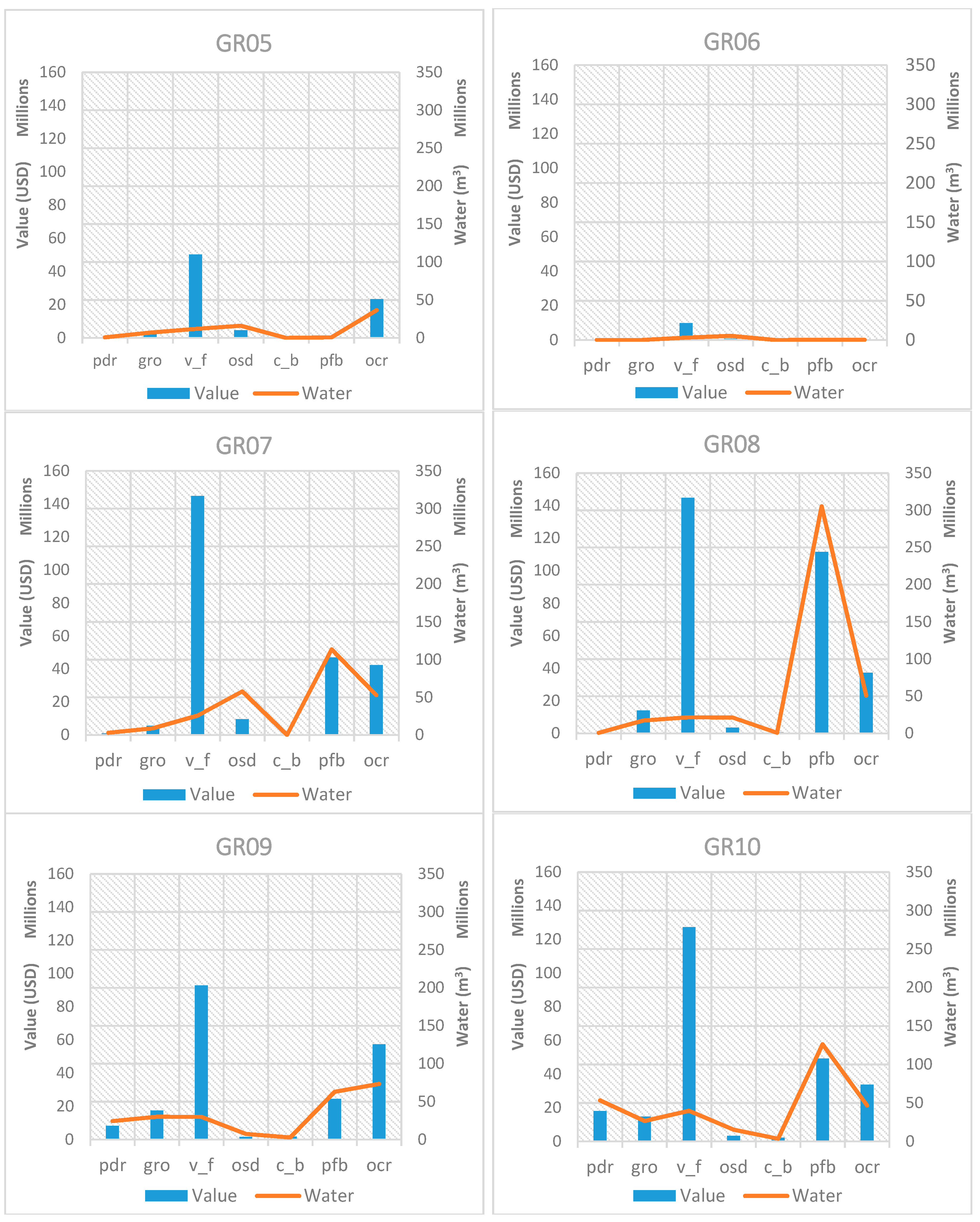
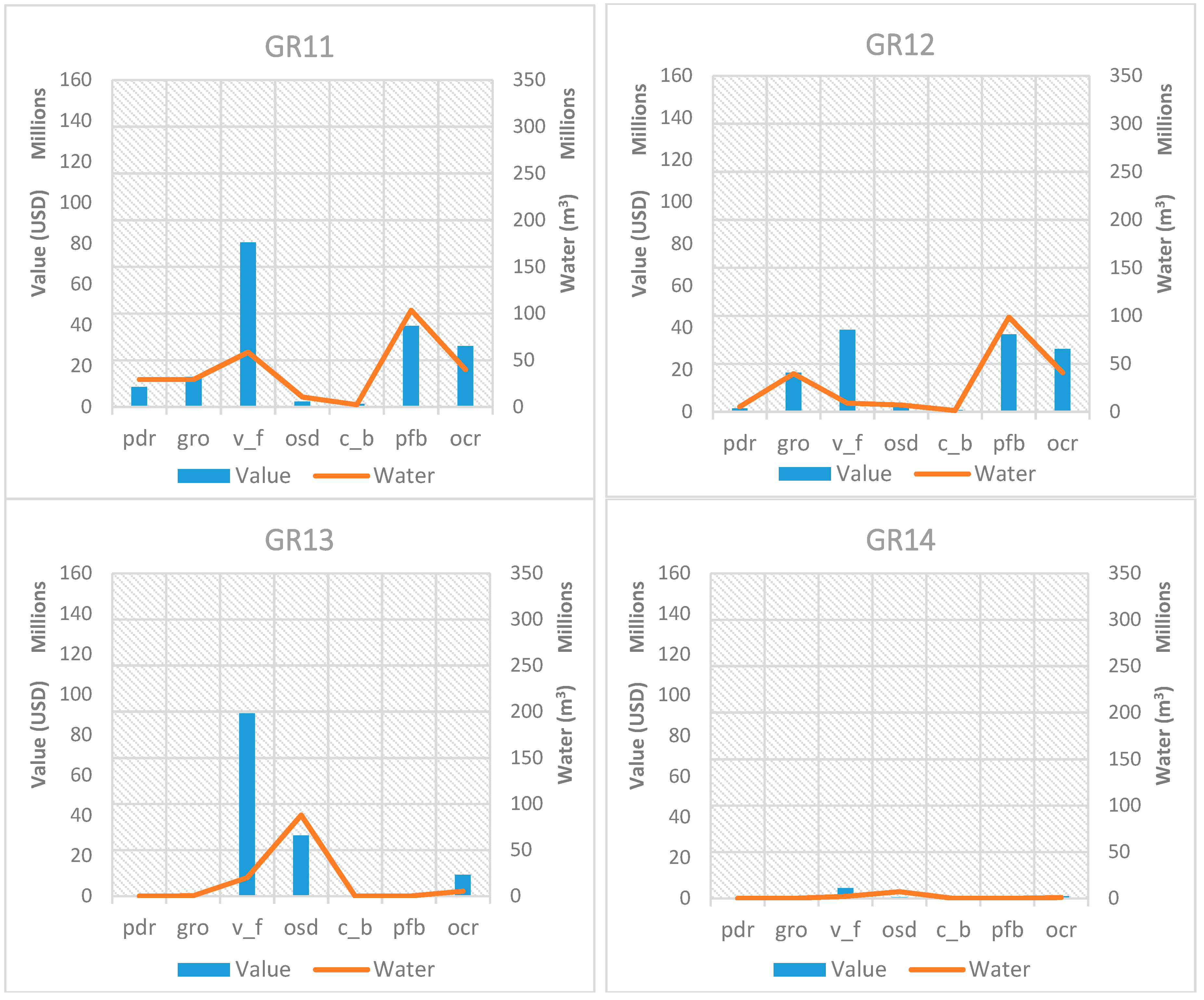
In order to assess the relationship between the value of exported crops and the associated virtual crop water exported, an analysis of the relationship of these two quantities is presented in Figure 5 for each RBD in Greece for 2011. In the presented graphs, the same scale is maintained on the axes, to facilitate a comparison among RBDs. The trends identified in Figure 4 are confirmed in these graphs, showing that wherever cotton (pfb) is produced, it dominates water exports. When comparing value and virtual crop water exported for cotton, it is important to note that water always exceeds associated value. The same is true for olives (osd), which are present in the Peloponnese (GR01, GR02 and GR03) and in Crete (GR13), even though the value and associated water are generally lower than those for cotton. Vegetables, fruit vegetables, and fruits & nuts which belong in the generic category “v_f” have the highest share value in all RBDs, while the associated virtual crop water exported is relatively low. Even though paddy rice (pdr), sugar beet (c_b), and maize, rye, oats and other cereals (all the latter grouped under the “gro” category) contribute with their corresponding share to the value of each RBD, they make up a set of agricultural products that export water quantities that exceed their relative value. Tobacco, alfalfa, clover, fodder root, and potatoes (grouped under the “ocr” category) have a relative value that exceeds their associated exported water.
4. Discussion
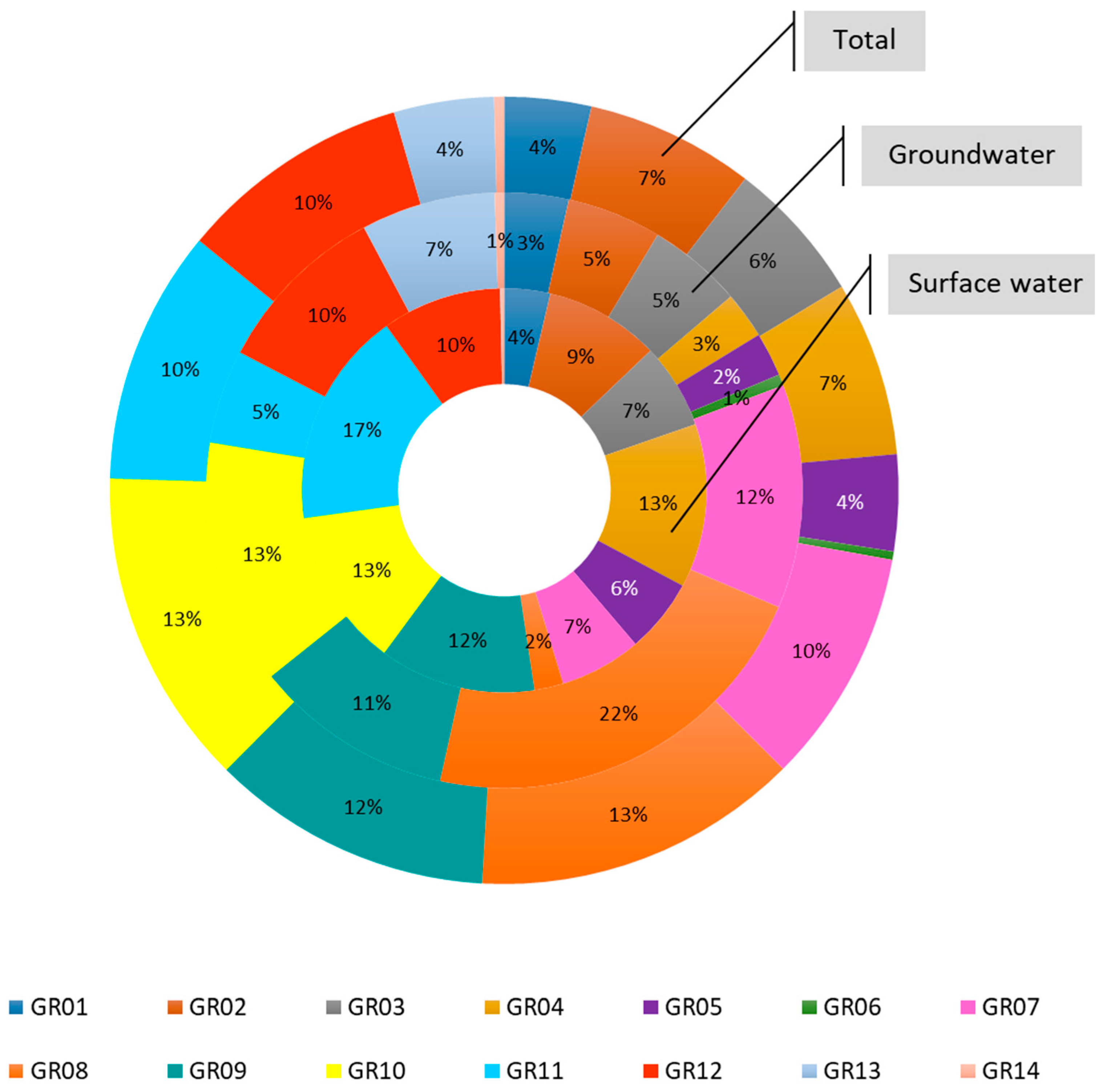
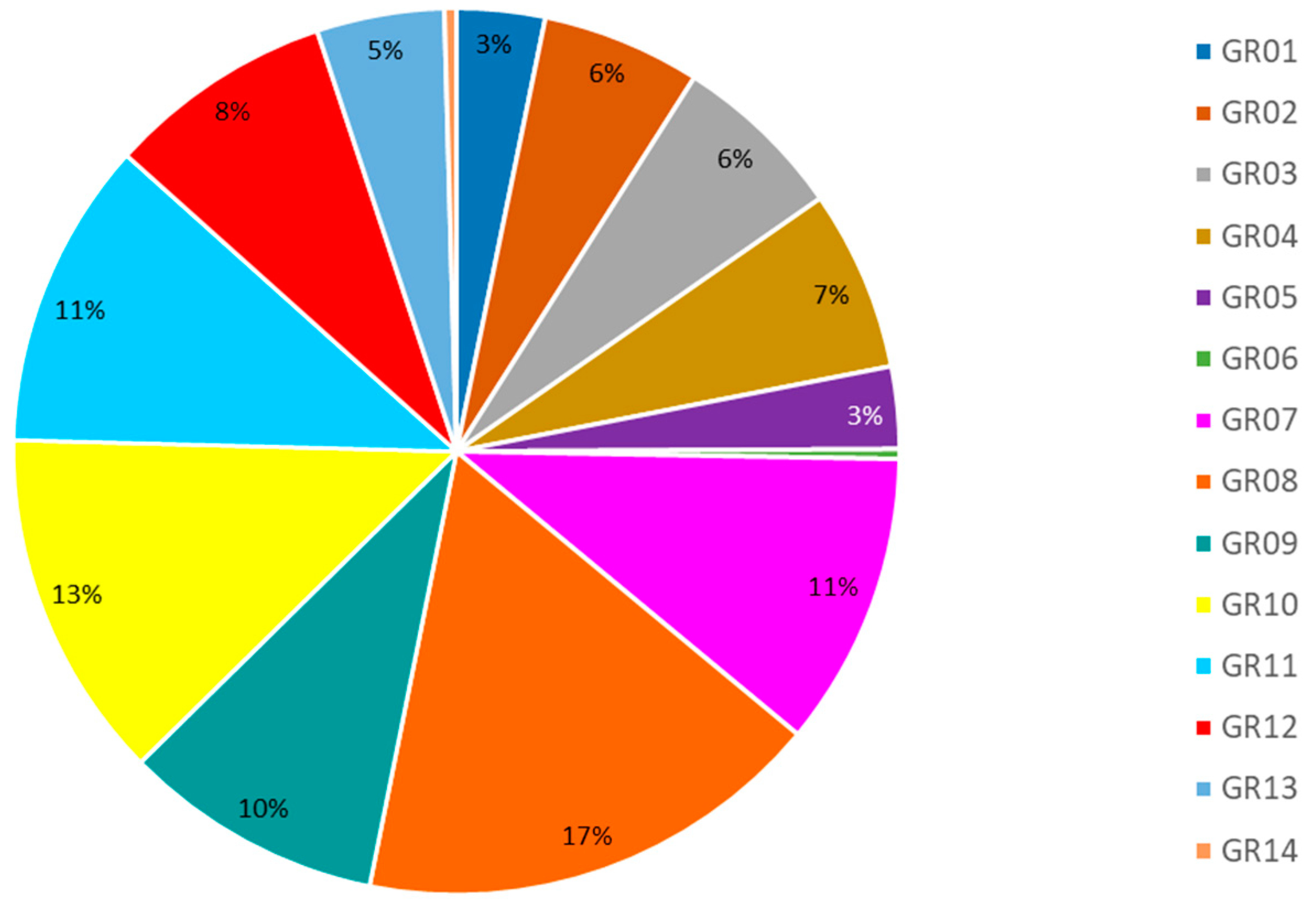
Agriculture is a considerable water consumer, impacting severely on water resources availability and thus, it is a subject of controversy regarding the formulation of agricultural policy aiming at relieving pressures on water resource. According to EUROSTAT, in Greece, a staggering 82% of total water is used by the agriculture sector; the same percentage applies to groundwater and surface water resources. In other words, 82% of both groundwater and surface water consumed in Greece, it is used by agricultural activities. When continuing with the analysis on the RBD level (Figure 6), the results are compelling, since it becomes evident that most of agricultural water comes from only a few RBDs and indeed from the ones that are highly stressed (GR08, GR09 and GR10); this reinforces what is shown in Figure 3. Furthermore, in Figure 6 we see that for GR08, almost all of agricultural water comes from groundwater, which, as we can see in Figure 1, is already characterized as “highly stressed” in terms of quantity by the Ministry. Given the fact that the largest agricultural water demand in the nation is exerted on GR08 and GR10 (Figure 6), it becomes obvious that these RBDs are under extreme stress. Furthermore, when it comes to virtual crop water exported, GR08 and GR10 are the ones with the highest virtual exported water quantities, as shown in Figure 7 and according to Figure 4, these trends are expected to intensify in consecutive years all the way to 2050.
Since the RBDs with the largest virtual water exports are the ones with the biggest problems in terms of water resource availability, the analysis of the value of exported crops is justified. If Greece faces water scarcity issues and consumes a large percentage of its water resources on agriculture and ends up exporting a significant part of agricultural products and thus their embedded water, at least it would be “comforting” to know that these exports have a high value for the Greek economy! Results from Figure 5 show that crops under the “v_f” category, namely vegetables, fruit vegetables, fruits and nuts are the most “promising” ones, since they are the ones that have the highest value on all RBDs, while their associated virtual water is proportionally very low. The analysis reveals that exporting crops under the “v_f” category will bring significant value to the economy, with the least water proportionally.
Naturally, it should be noted that this result is based solely on the amount of virtual crop water embedded in the crops and it does not consider other inputs in this crop type, such as energy, labor, land, soil, fertilizers, pesticides, etc. Furthermore, this analysis does not consider the other part of the equation, which is the water embedded in the imported products into these RBDs, which may bring water savings into the water stressed regions as well. Such analysis goes beyond the scope of this article and would be a valuable continuation of this work. The procedure of estimating the total crop exports (including indirect exports) using value of domestic input and export shares has a number of caveats that should be considered. The most important is that aggregate sectors in MAGNET might hide the non-homogeneous characteristics of individual crops and food sectors. In other words, even though under the crop category “v_f” there are several crops with different water demands, we are not able to track which specific crops are being exported, but we base our calculations on average values. Moreover, we assume that all inputs into the exporting sector are exported in equal measure. In the same way, the “Services” and “Other industry” sectors include many outputs that do not use food as an input, even though the aggregate sector does use food inputs. For the former, we have used the conservative estimate that all service exports were of labor and expertise and not of physical food, even though the “services” sector purchases inputs from crops. Similarly, we assumed that inputs into food sectors from the latter sector did not include any indirect crops, so “Other industry” was left out of the set di1 in the Appendix. Nevertheless, even after considering these important caveats, we believe that the method of estimating the total crop exports, as presented in this article, is reasonable and sound.
To compare throughout all RBDs and all crop types, Table 4 is included, which shows the relationship between value and virtual exported water. The exported virtual crop water per value ratio presented as “unit of virtual crop water (m3) per USD” shows that vegetables and fruits are the most advantageous crops from an economic and a water perspective, when considered together, since the said ratio has the lowest value for all RBDs. Cotton, the largest virtual crop water exporter in Greece appears much less advantageous, since the ratios have relatively large values, as shown in Table 4. Even though the ratios are not the largest for cotton, their relative size is significant since the water volumes are much larger than in other crops. For comparison purposes, the water to value ratio has a really high value (9.88) in GR14 for paddy rice (pdr). However, as we see in Figure 5, water volumes in this RBD are so low that such a high number is less significant. Olives (osd) also appear to have relatively high ratios, deeming them less advantageous in terms of value and virtual crop water exported. Figure 8 shows a graphical representation of the water to value ratio for all RBDs, in order to show its variation throughout the RBDs. As mentioned before, these ratios should only be considered along with the graphs in Figure 5, which show the intensity of water use in each RBD, in order to identify the most significant crops.
Author Contributions
C.L. and N.M. conceived the concept of the article; J.L.K. performed MAGNET model runs and provided relevant data. N.M. calculated water demands for all crops and conducted analysis with MAGNET data. C.L. and N.M. wrote the paper with input from J.L.K. All authors reviewed the final manuscript.
Funding
The work described in this paper has been conducted within the project SIM4NEXUS. This project has received funding from the European Union’s Horizon 2020 research and innovation programme under Grant Agreement No. 689150 SIM4NEXUS. This paper and the content included in it do not represent the opinion of the European Union, and the European Union is not responsible for any use that might be made of its content.
Acknowledgments
We would like to thank Marijke Kuiper for some useful methodological discussions and her editing suggestions. We also thank two anonymous reviewers whose comments contributed to significantly improving the quality of this paper.
Conflicts of Interest
The authors declare no conflict of interest.
Appendix A

Table A1.
Set definition for sector sets used in Formulas (1)–(4).
| Set Name | Crops | Direct Inputs | Direct Inputs Less Processed Foods and Other Industry | Animals | Meat | Processed Food |
|---|---|---|---|---|---|---|
| Set symbol | c | di | di1 | an | mt | proF |
| Includes sectors | Paddy rice | Cattle | Cattle | Cattle | Cattle meat | Processed food |
| Wheat | Dairy cows | Dairy cows | Dairy cows | Other meat | ||
| Other grains | Other animals | Other animals | Other animals | |||
| Vegetables and fruits | Cattle meat | Cattle meat | ||||
| Oil seeds | Other meat | Other meat | ||||
| Sugar beets | Sugar | Sugar | ||||
| Plant-based fibers | Vegetable oil | Vegetable oil | ||||
| Other crops | Processed rice | Processed rice | ||||
| Processed food | Animal feed | |||||
| Animal feed | ||||||
| Other industry |
References
- European Commission. Communication from the Commission to the European Parliament, the Council, the European Economic and Social Committee and the Committee of the Regions. A Resource-Efficient Europe—Flagship Initiative under the Europe 2020 Strategy; COM(2011) 21; European Commission: Brussels, Belgium, 2011. [Google Scholar]
- WWDR4—Background Information Brief. Available online: http://www.unesco.org/new/fileadmin/MULTIMEDIA/HQ/SC/pdf/WWDR4%20Background%20Briefing%20Note_ENG.pdf (accessed on 2 February 2018).
- National Footprint Accounts, 2012 Edition. Available online: http://www.footprintnetwork.org/images/article_uploads/National_Footprint_Accounts_2012_Edition_Report.pdf (accessed on 1 February 2018).
- Mohtar, R.H.; Daher, B. Water, Energy, and Food: The Ultimate Nexus. In Encyclopedia of Agricultural, Food, and Biological Engineering, 2nd ed.; Heldman, D., Moraru, C., Eds.; CRC Press: Boca Raton, FL, USA, 2010; ISBN 9781439811115/1439811113. [Google Scholar]
- Ahuja, S. Overview: Sustaining Water, the World’s Most Crucial Resource. In Chemistry and Water the Science behind Sustaining the World’s Most Crucial Resource; Ahuja, S., Ed.; Elsevier: New York, NY, USA, 2017; pp. 1–22. ISBN 978-0-12-809330-6. [Google Scholar]
- Hoekstra, A.Y.; Hung, P.Q. Globalisation of water resources: International virtual water flows in relation to crop trade. Glob. Environ. Chang. 2005, 15, 45–56. [Google Scholar] [CrossRef]
- Vörösmarty, C.J.; Hoekstra, A.Y.; Bunn, S.E.; Conway, D.; Gupta, J. Fresh water goes global. Science 2015, 349, 478–479. [Google Scholar] [CrossRef] [PubMed] [Green Version]
- Mekonnen, M.M.; Hoekstra, A.Y. A global assessment of the water footprint of farm animal products. Ecosystems 2012, 15, 401–415. [Google Scholar] [CrossRef]
- Laspidou, C.S. Grey water footprint of crops and crop-derived products: Analysis of calculation method. Fresenius Environ. Bull. 2014, 23, 2899–2903. [Google Scholar]
- Hoekstra, A.Y.; Hung, P.Q. Virtual water trade: A quantification of virtual water flows between nations in relation to international crop trade. In Value of Water: Research Report Series No.11; UNESCO-IHE: Delft, The Netherlands, 2002. [Google Scholar]
- Zimmer, D.; Renault, D. Virtual water in food production and global trade: Review of methodological issues and preliminary results. In Virtual Water Trade, Proceedings of the International Expert Meeting on Virtual Water Trade, Value of Water Research Report Series, Delft, The Netherlands, 12–13 December 2003; UNESCOIHE Institute for Water Education: Delft, The Netherlands, 2003; Volume 12, pp. 1–19. [Google Scholar]
- Guan, D.; Hubacek, K. Assessment of regional trade and virtual water flows in China. Ecol. Econ. 2007, 61, 159–170. [Google Scholar] [CrossRef]
- Allan, J.A. Virtual water—Economically invisible and politically silent—A way to solve strategic water problems. Int. Water Irrig. 2001, 21, 39–41. [Google Scholar]
- Karavitis, C.A.; Kerkides, P. Estimation of the water resources potential in the island system of the Aegean Archipelago, Greece. Water Int. 2002, 27, 243–254. [Google Scholar] [CrossRef]
- Nastos, P.T.; Zerefos, C.S. Climate change and precipitation in Greece. Hellenic J. Geosci. 2010, 45, 185–192. [Google Scholar]
- Woltjer, G.; Kuiper, M.; Kavallari, A.; van Meijl, H.; Powell, J.; Rutten, M.; Shutes, L.; Tabeau, A. The MAGNET Model—Module Description; LEI Report 14-057; LEI—Part of Wageningen UR: The Hague, The Netherlands, 2014. [Google Scholar]
- Hertel, T. Global Trade Analysis: Modelling and Applications; Cambridge University Press: Cambridge, UK, 1997; p. 403. [Google Scholar]
- Stehfest, E.; van Vuuren, D.; Bouwman, L.; Kram, T. Integrated Assessment of Global Environmental Change with IMAGE 3.0: Model Description and Policy Applications; Environmental Assessment Agency (PBL): The Hague, The Netherlands, 2014; pp. 32–54. ISBN 978-94-91506-71-0. [Google Scholar]
- O’Neill, B.C.; Kriegler, E.; Ebi, K.L.; Kemp-Benedict, E.; Riahi, K.; Rothman, D.S.; van Ruijven, J.; van Vuuren, D.P.; Birkmann, J.; Kok, K.; et al. The roads ahead: Narratives for shared socioeconomic pathways describing world futures in the 21st century. Glob. Environ. Chang. 2017, 42, 169–180. [Google Scholar] [CrossRef]
- Van Meijl, H.; Havlik, P.; Lotze-Campen, H.; Stehfest, E.; Witzke, P.; Pérez Domínguez, I.; Bodirsky, B.; van Dijk, M.; Doelman, J.; Fellmann, T.; et al. Challenges of Global Agriculture in a Climate Change Context by 2050 (AgCLIM50); JRC Science for Policy Report; EUR 28649 EN, Publications Office of the European Union: Luxembourg, 2017; ISBN 978-92-79-69666-4. [Google Scholar]
- Hellenic Statistical Authority. Areas and Production. 2011. Available online: http://www.statistics.gr/el/statistics/-/publication/SPG06/2011 (accessed on 26 October 2017). (In Greek).
- Institute of Agricultural Research of Cyprus. Calculation of Monthly Water Demand per Location and Crop. Available online: http://news.ari.gov.cy/irrigation_v1.html (accessed on 15 April 2017). (In Greek).
- European Environment Agency Crop Water Demand. Available online: https://www.eea.europa.eu/data-and-maps/indicators/water-requirement-2/assessment (accessed on 10 April 2018).
Figure 1.
A map of Greece illustrating groundwater stress levels for all RBDs (adjusted from data obtained by the Hellenic Ministry of the Environment and Climate Change, nmwn.ypeka.gr/map).
Figure 1.
A map of Greece illustrating groundwater stress levels for all RBDs (adjusted from data obtained by the Hellenic Ministry of the Environment and Climate Change, nmwn.ypeka.gr/map).
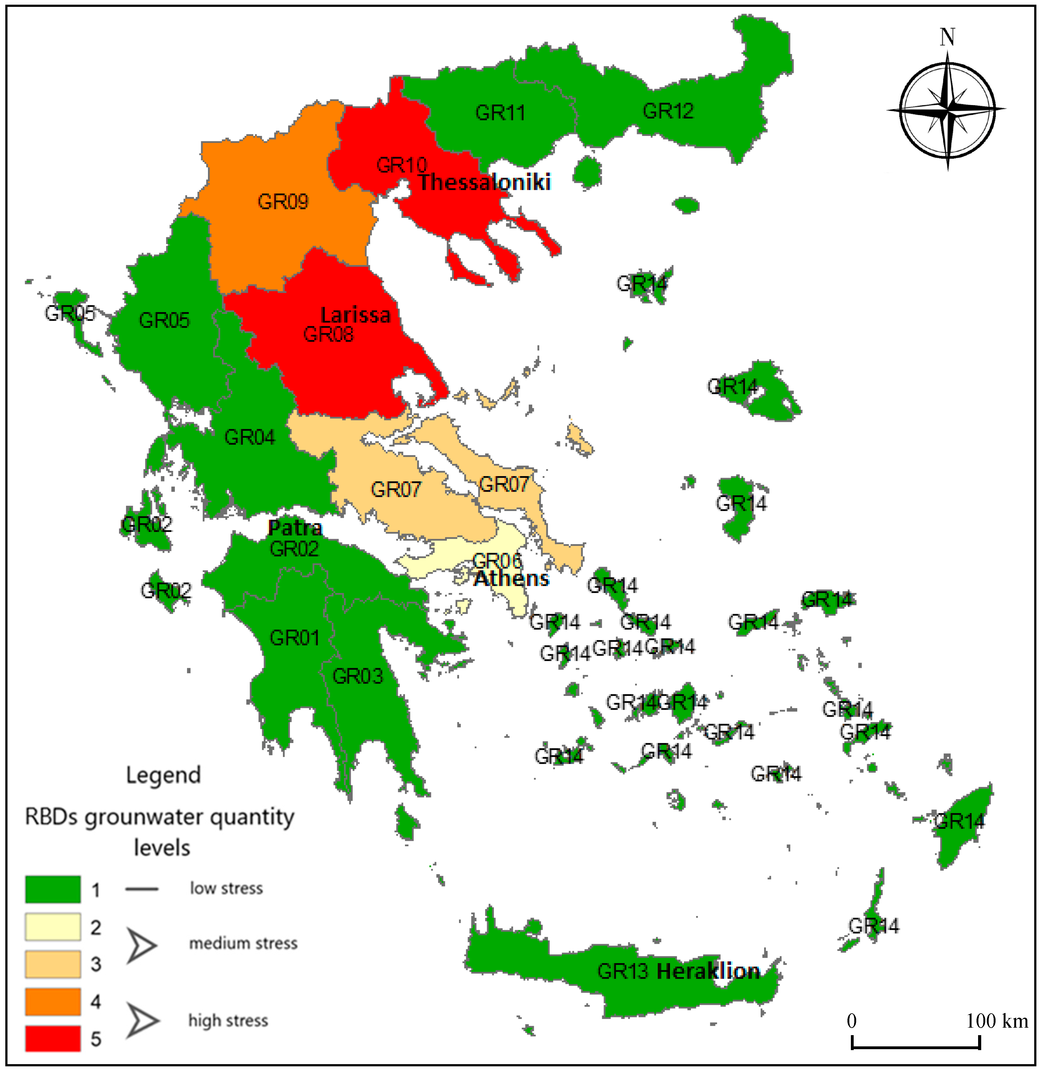
Figure 2.
Total crop export including indirect exports from the noncrop sectors. The numbers in the brackets indicate the equation number that describes the corresponding product.
Figure 2.
Total crop export including indirect exports from the noncrop sectors. The numbers in the brackets indicate the equation number that describes the corresponding product.

Figure 3.
The amount of irrigation water consumed in Greek territory (locally used) against exported through trade and the percentage contribution to the exported water downscaled to low-, highly and medially stressed RBD areas.
Figure 3.
The amount of irrigation water consumed in Greek territory (locally used) against exported through trade and the percentage contribution to the exported water downscaled to low-, highly and medially stressed RBD areas.

Figure 4.
The two crop types with the highest virtual crop water exported per RBD in Greece for years 2011, 2030 and 2050. Reported numbers are in thousands of cubic meters of water.
Figure 4.
The two crop types with the highest virtual crop water exported per RBD in Greece for years 2011, 2030 and 2050. Reported numbers are in thousands of cubic meters of water.

Figure 5.
Exported crop values in comparison with the corresponding virtual crop water for all RBDs in Greece for the base year 2011.
Figure 5.
Exported crop values in comparison with the corresponding virtual crop water for all RBDs in Greece for the base year 2011.


Figure 6.
Distribution of agricultural water demand on Greek RBDs, with a distinction between groundwater and surface water for base year 2011.
Figure 6.
Distribution of agricultural water demand on Greek RBDs, with a distinction between groundwater and surface water for base year 2011.

Figure 7.
Distribution of exported virtual crop water on Greek RBDs, for base year 2011.

Figure 8.
Variation of exported virtual crop water per value ratio for all crop types and all RBDs in Greece for base year 2011 (in m3 of virtual crop water per USD).
Figure 8.
Variation of exported virtual crop water per value ratio for all crop types and all RBDs in Greece for base year 2011 (in m3 of virtual crop water per USD).

Table 1.
Crop category codes used in MAGNET, types of crops included under each category and the corresponding quantities in 2011, used as input to MAGNET.
Table 1.
Crop category codes used in MAGNET, types of crops included under each category and the corresponding quantities in 2011, used as input to MAGNET.
| Generic Crop Category Codes | Quantities in Metric Tons | Types of Crops | Quantities in Metric Tons |
|---|---|---|---|
| pdr | 219,200 | paddy rice | 219,200 |
| gro | 1,993,584 | maize rye oats other cereals | 1,781,072 26,794 66,379 119,339 |
| v_f | 4,430,959 | vegetables fruit vegetables fruit & nuts | 780,268 1,195,693 2,454,997 |
| osd | 731,536 | olives | 731,536 |
| c_b | 490,508 | sugar beet | 490,508 |
| pfb | 631,867 | cotton | 631,867 |
| ocr | 1,965,601 | tobacco alfalfa clover fodder root potatoes | 26,997 1,167,928 121,719 6 648,951 |
Table 2.
Crop production market values in 2011, 2030 and 2050.
| Generic Crop Categories | 2011 Production Values in Constant 2011 Million USD | 2030 Production Values in Constant 2011 Million USD | 2050 Production Values in Constant 2011 Million USD |
|---|---|---|---|
| pdr | 119.31 | 117.05 | 128.22 |
| gro | 897.39 | 970.77 | 1024.91 |
| v_f | 5578.1 | 5590.00 | 5779.61 |
| osd | 302.08 | 330.34 | 363.59 |
| c_b | 32.39 | 23.08 | 21.84 |
| pfb | 619.59 | 670.79 | 745.63 |
| ocr | 1686.08 | 1715.54 | 1867.05 |
Table 3.
Total exports value of the crops in 2011, 2030, and 2050 in constant 2011 prices.
| Generic Crop Categories | Total Exports Value (Millions USD) in 2011 | Total Exports Value (Millions USD) in 2030 | Total Exports Value (Millions USD) in 2050 |
|---|---|---|---|
| pdr | 40.05 | 38.91 | 50.65 |
| gro | 107.62 | 122.27 | 131.24 |
| v_f | 1252.70 | 1266.17 | 1435.23 |
| osd | 121.54 | 136.50 | 154.94 |
| c_b | 6.89 | 2.78 | 3.21 |
| pfb | 334.69 | 373.59 | 428.46 |
| ocr | 369.59 | 391.75 | 516.49 |
Table 4.
Exported virtual crop water per value ratio for all crop types and all RBDs in Greece for base year 2011 (in m3 of virtual crop water per USD). Shaded cells represent the lowest values.
Table 4.
Exported virtual crop water per value ratio for all crop types and all RBDs in Greece for base year 2011 (in m3 of virtual crop water per USD). Shaded cells represent the lowest values.
| Crops | GR01 | GR02 | GR03 | GR04 | GR05 | GR06 | GR07 | GR08 | GR09 | GR10 | GR11 | GR12 | GR13 | GR14 |
|---|---|---|---|---|---|---|---|---|---|---|---|---|---|---|
| pdr | 4.35 | 4.35 | 4.73 | 4.00 | 3.02 | 3.70 | 3.26 | 2.98 | 2.96 | 2.96 | 2.99 | 3.47 | 0 | 9.88 |
| gro | 2.16 | 2.22 | 3.04 | 1.86 | 1.88 | 1.01 | 1.60 | 1.24 | 1.73 | 1.80 | 2.01 | 2.14 | 3.02 | 0.22 |
| v_f | 0.27 | 0.26 | 0.30 | 0.21 | 0.24 | 0.30 | 0.18 | 0.15 | 0.32 | 0.31 | 0.73 | 0.23 | 0.22 | 0.43 |
| osd | 3.37 | 2.73 | 3.56 | 3.42 | 3.50 | 7.30 | 6.12 | 6.05 | 4.56 | 4.55 | 4.11 | 3.23 | 2.93 | 11.66 |
| c_b | 0 | 0 | 0 | 1.36 | 1.68 | 1.48 | 1.30 | 1.43 | 1.68 | 1.68 | 1.67 | 1.62 | 0 | 9.89 |
| pfb | 2.02 | 2.02 | 2.33 | 2.50 | 2.57 | 2.36 | 2.42 | 2.74 | 2.57 | 2.57 | 2.61 | 2.68 | 0 | 1.48 |
| ocr | 0.84 | 0.95 | 1.24 | 1.06 | 1.56 | 0.56 | 1.25 | 1.37 | 1.28 | 1.38 | 1.34 | 1.36 | 0.51 | 0.94 |
© 2018 by the authors. Licensee MDPI, Basel, Switzerland. This article is an open access article distributed under the terms and conditions of the Creative Commons Attribution (CC BY) license (http://creativecommons.org/licenses/by/4.0/).
Share and Cite
MDPI and ACS Style
Mellios, N.; Koopman, J.F.L.; Laspidou, C. Virtual Crop Water Export Analysis: The Case of Greece at River Basin District Level. Geosciences 2018, 8, 161. https://doi.org/10.3390/geosciences8050161
AMA Style
Mellios N, Koopman JFL, Laspidou C. Virtual Crop Water Export Analysis: The Case of Greece at River Basin District Level. Geosciences. 2018; 8(5):161. https://doi.org/10.3390/geosciences8050161
Chicago/Turabian StyleMellios, Nikolaos, Jason F. L. Koopman, and Chrysi Laspidou. 2018. "Virtual Crop Water Export Analysis: The Case of Greece at River Basin District Level" Geosciences 8, no. 5: 161. https://doi.org/10.3390/geosciences8050161
Note that from the first issue of 2016, this journal uses article numbers instead of page numbers. See further details here.