Numerically Calculated 3D Space-Weighting Functions to Image Crustal Volcanic Structures Using Diffuse Coda Waves

 ,
,  ,
,  , , and
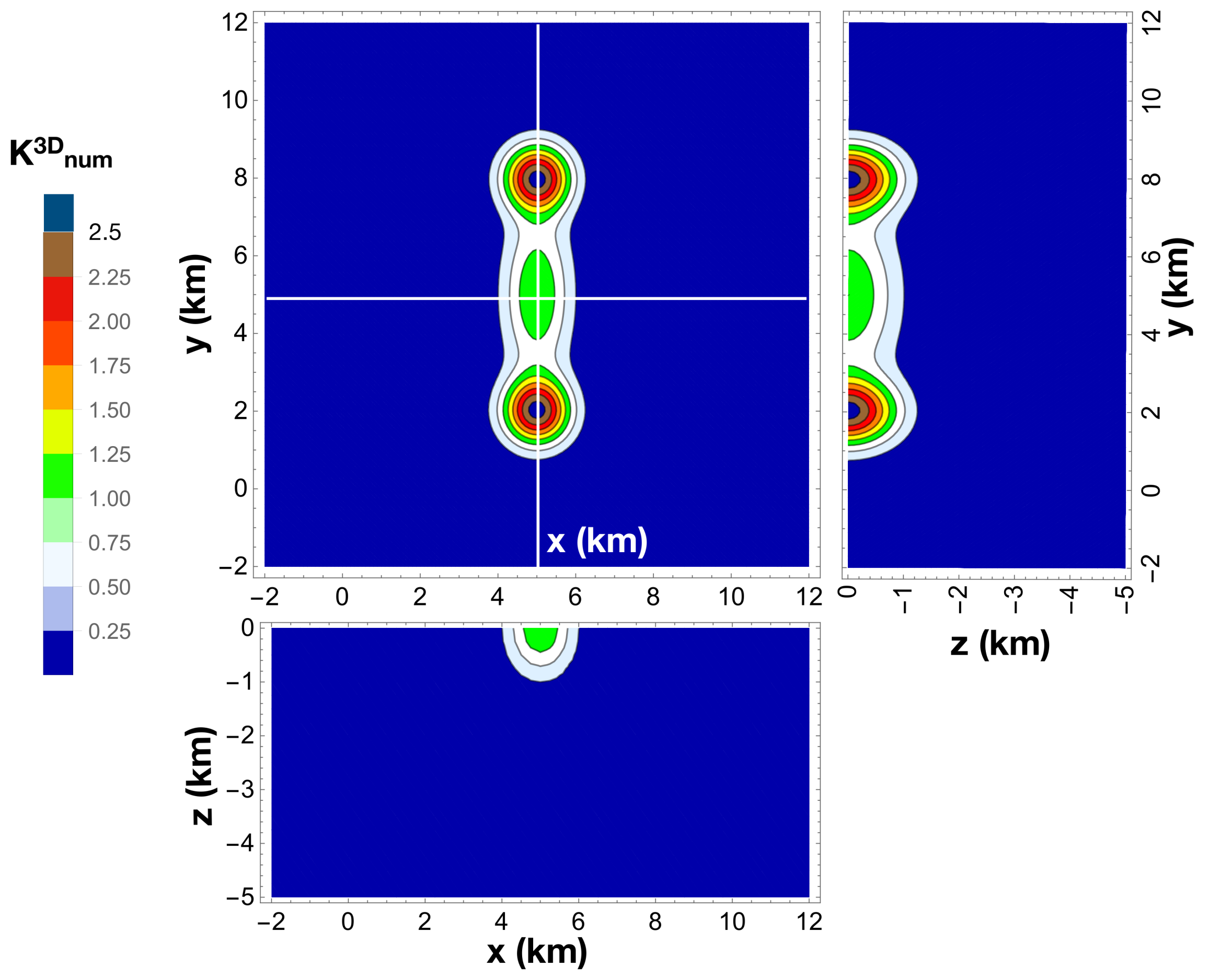
Abstract
1. Introduction
- Equation (4) is extended to the third dimension, maintaining the assumptions of shallow source and receiver in a diffusive Earth medium with no depth dependency—this is the case for the analysis of active seismic shots in volcanoes.
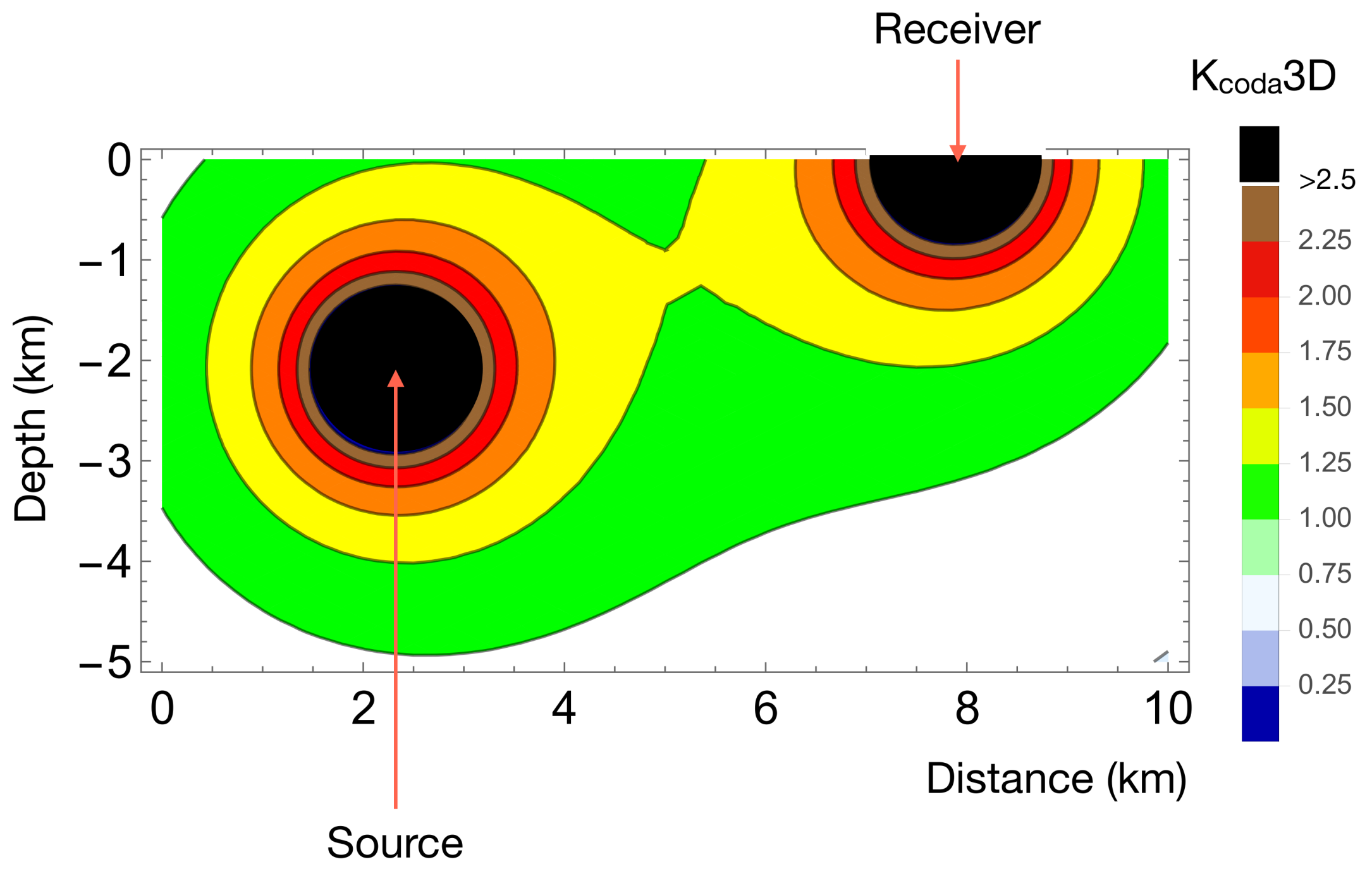
- We propose and discuss an SWF for mapping , calculated for a deep source in a non-diffusive medium and discuss its limits.
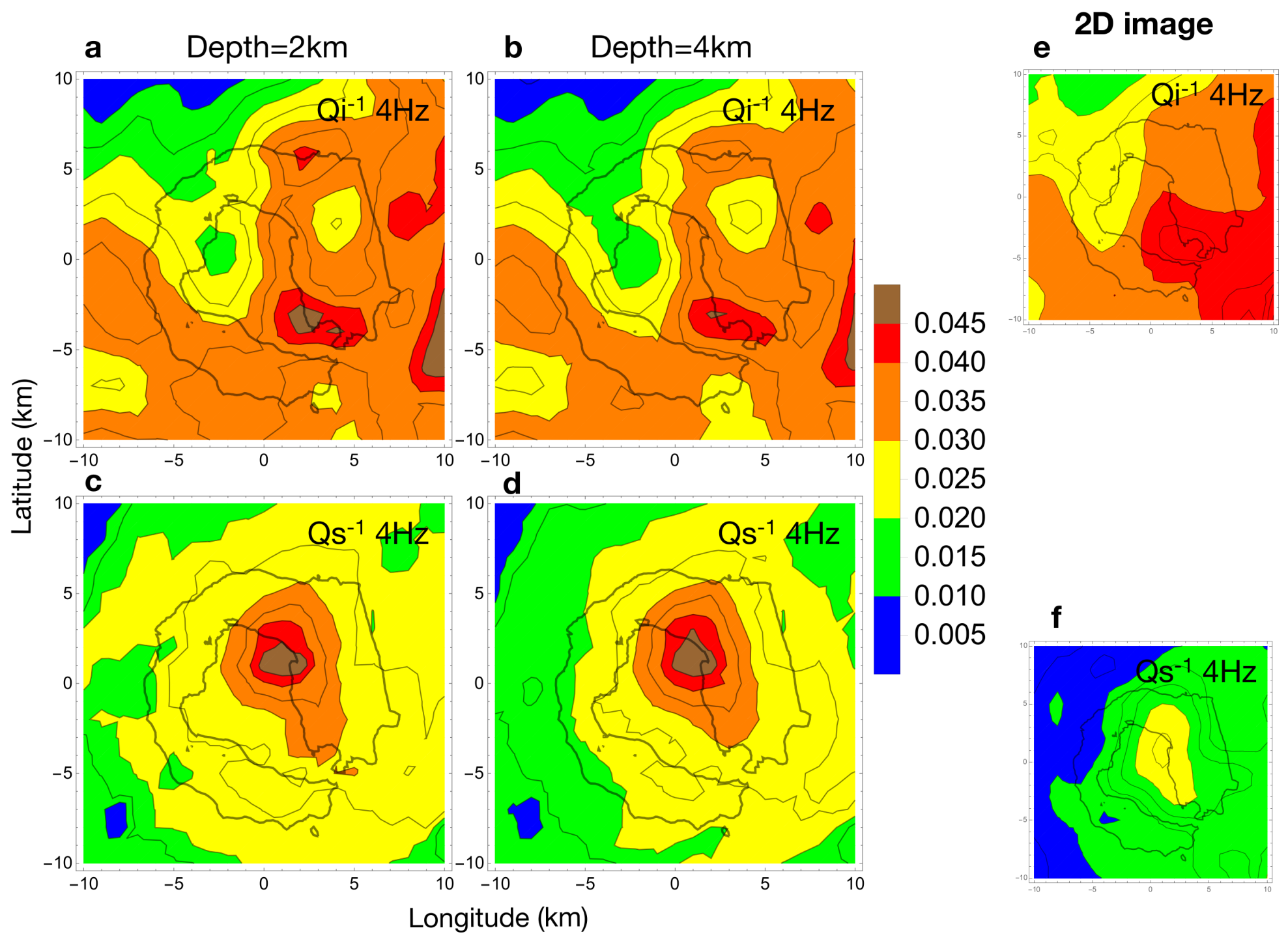
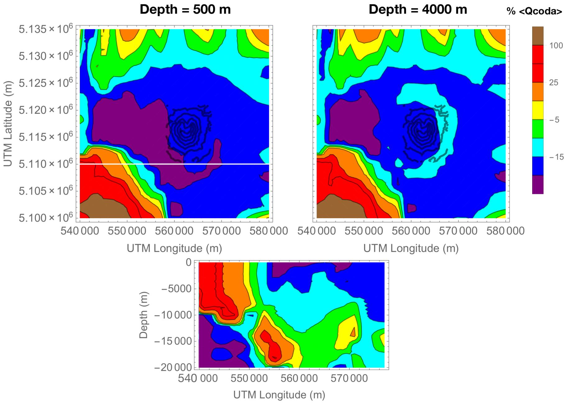
- We check the reliability and limits of the new approaches by applying 3D SWFs to published seismic databases. We use precalculated attenuation measurements for single source station paths from active data recorded at the Deception Island volcano (Antarctica) [21] and volcano tectonic earthquakes at the Mount St. Helens volcano (USA) [22].
2. Results
2.1. 3D Extension of the 2D Weighting Functions
2.1.1. Diffusive Earth Media
2.1.2. Deep Sources (Natural Events) and Non-Diffusive Fields
2.2. Application Examples
- The values of express the probability that the estimated at a station is equal to the one measured at [x, y, z].
- Equation (9) is to be used exclusively for back-projection.
- The kernel in Equation (5) can still be used in an inversion for the space-dependent parameters, if the underlying hypotheses are fulfilled.
2.2.1. Deception Island Volcano—Diffusive Approximation
2.2.2. 3D SWF at Mount St. Helens Volcano—Non-Diffusive Media
3. Discussion
Author Contributions
Acknowledgments
Conflicts of Interest
Abbreviations
| SWF | Space-Weighted Functions |
Appendix A. Demonstration that Approaches in Media with Small

Appendix B. Sensitivity Tests for 3D SWF


Appendix C. Numerical Integration of Equation (8)
References
- Calvet, M.; Sylvander, M.; Margerin, L.; Villasenor, A. Spatial variations of seismic attenuation and heterogeneity in the Pyrenees: Coda Q and peak delay time analysis. Tectonophysics 2013, 608, 428–439. [Google Scholar] [CrossRef]
- Mayor, J.; Calvet, M.; Margerin, L.; Vanderhaeghe, O.; Traversa, P. Crustal structure of the Alps as seen by attenuation tomography. Earth Planet. Sci. Lett. 2016, 439, 71–80. [Google Scholar] [CrossRef]
- De Siena, L.; Calvet, M.; Watson, K.J.; Jonkers, A.R.T.; Thomas, C. Seismic scattering and absorption mapping of debris flows, feeding paths, and tectonic units at Mount St. Helens volcano. Earth Planet. Sci. Lett. 2016, 442, 21–31. [Google Scholar] [CrossRef]
- Prudencio, J.; Del Pezzo, E.; Ibanez, J.; Giampiccolo, E.; Patane, D. Two-dimensional seismic attenuation images of Stromboli Island using active data. Geophys. Res. Lett. 2015, 42, 1717–1724. [Google Scholar] [CrossRef]
- Del Pezzo, E.; Ibáñez, J.; Morales, J.; Akinci, A.; Maresca, R. Measurements of intrinsic and scattering seismic attenuation in the crust. Bull. Seismol. Soc. Am. 1995, 85, 1373–1380. [Google Scholar]
- Akinci, A.; Del Pezzo, E.; Ibañez, J. Separation of scattering and intrinsic attenuation in the Southern Spain and Western Anatolia (Turkey). Geophys. J. Int. 1995, 121, 337–353. [Google Scholar] [CrossRef]
- Wegler, U.; Luhr, B. Scattering behaviour at Merapi volcano(Java) revealed from an active seismic experiment. Geophys. J. Int. 2001, 145, 579–592. [Google Scholar] [CrossRef]
- Lacombe, C.; Campillo, M.; Paul, A.; Margerin, L. Separation of intrinsic absorption and scattering attenuation from Lg coda decay in central France using acoustic radiative transfer theory. Geophys. J. Int. 2003, 154, 417–425. [Google Scholar] [CrossRef]
- Xie, J.; Mitchell, B. A back-projection method for imaging lLarge-scale lateral variations of Lg Coda Q with application to Continental Africa. Geophys. J. Int. 1990, 100, 161–181. [Google Scholar] [CrossRef]
- Margerin, L.; Planes, T.; Mayor, J.; Calvet, M. Sensitivity kernels for coda-wave interferometry and scattering tomography: Theory and numerical evaluation in two-dimensional anisotropically scattering media. Geophys. J. Int. 2016, 204, 650–666. [Google Scholar] [CrossRef]
- Rossetto, V.; Margerin, L.; Planès, T.; Larose, É. Locating a weak change using diffuse waves (LOCADIFF): Theoretical approach and inversion procedure. arxiv, 2010; arXiv:1007.3103. [Google Scholar]
- Obermann, A.; Planès, T.; Larose, E.; Sens-Schönfelder, C.; Campillo, M. Depth sensitivity of seismic coda waves to velocity perturbations in an elastic heterogeneous medium. Geophys. J. Int. 2013, 194, 372–382. [Google Scholar] [CrossRef]
- Singh, S.; Herrmann, R.B. Regionalization of Crustal Coda Q in the continental United States. J. Geophys. Res. 1983, 88, 527–538. [Google Scholar] [CrossRef]
- Yoshimoto, K. Monte Carlo simulation of seismogram envelopes in scattering media. J. Geophys. Res. 2000, 105, 6153–6161. [Google Scholar] [CrossRef]
- Prudencio, J.; Del Pezzo, E.; Garcia Yeguas, A.; Ibanez, J.M. Spatial distribution of intrinsic and scattering seismic attenuation in active volcanic islands—I: Model and the case of Tenerife Island. Geophys. J. Int. 2013, 195, 1942–1956. [Google Scholar] [CrossRef]
- Prudencio, J.; Ibanez, J.M.; Garcia Yeguas, A.; Del Pezzo, E.; Posadas, A.M. Spatial distribution of intrinsic and scattering seismic attenuation in active volcanic islands—II: Deception Island images. Geophys. J. Int. 2013, 195, 1957–1969. [Google Scholar] [CrossRef]
- Del Pezzo, E.; Ibañez, J.; Prudencio, J.; Bianco, F.; De Siena, L. Absorption and scattering 2-D volcano images from numerically calculated space-weighting functions. Geophys. J. Int. 2016, 206, 742–756. [Google Scholar] [CrossRef][Green Version]
- Sato, H. Study of seismogram envelopes based on scattering by random inhomogeneities in the lithosphere: A review. Phys. Earth Planet. Inter. 1991, 67, 4–19. [Google Scholar] [CrossRef]
- Hoshiba, M. Simulation Of Multiple-scattered Coda Wave Excitation Based On The Energy-conservation Law. Phys. Earth Planet. Inter. 1991, 67, 123–136. [Google Scholar] [CrossRef]
- De Siena, L.; Amoruso, A.; Pezzo, E.D.; Wakeford, Z.; Castellano, M.; Crescentini, L. Space-weighted seismic attenuation mapping of the aseismic source of Campi Flegrei 1983–1984 unrest. Geophys. Res. Lett. 2017, 44, 1740–1748. [Google Scholar]
- Ibañez, J.M.; Díaz-Moreno, A.; Prudencio, J.; Zandomeneghi, D.; Wilcock, W.; Barclay, A.; Almendros, J.; Benítez, C.; García-Yeguas, A.; Alguacil, G. Database of multi-parametric geophysical data from the TOMO-DEC experiment on Deception Island, Antarctica. Sci. Data 2017, 4, 170128. [Google Scholar] [CrossRef] [PubMed]
- De Siena, L.; Thomas, C.; Aster, R. Multi-scale reasonable attenuation tomography analysis (MuRAT): An imaging algorithm designed for volcanic regions. J. Volcanol. Geotherm. Res. 2014, 277, 22–35. [Google Scholar] [CrossRef]
- Paasschens, J. Solution of the time-dependent Boltzmann equation. Phys. Rev. E 1997, 56, 1135–1141. [Google Scholar] [CrossRef]
- Zeng, Y.; Su, F.; Aki, K. Scattering wave energy propagation in a random isotropic scattering medium. Part 1. Theory. J. Geophys. Res. Solid Earth 1991, 96, 607–619. [Google Scholar] [CrossRef]
- Sato, H. Single isotropic scattering model including wave convesions Simple theoretical model of the short period body wave propagation. J. Phys. Earth 1977, 25, 163–176. [Google Scholar] [CrossRef]
- Pacheco, C.; Snieder, R. Time-lapse travel time change of multiply scattered acoustic waves. J. Acoust. Soc. Am. 2005, 118, 1300–1310. [Google Scholar] [CrossRef]
- De Siena, L.; Thomas, C.; Waite, G.P.; Moran, S.C.; Klemme, S. Attenuation and scattering tomography of the deep plumbing system of Mount St. Helens. J. Geophys. Res. Solid Earth 2014, 119, 8223–8238. [Google Scholar] [CrossRef]
- Ben-Zvi, T.; Wilcock, W.S.D.; Barclay, A.H.; Zandomeneghi, D.; Ibanez, J.M.; Almendros, J. The P-wave velocity structure of Deception Island, Antarctica, from two-dimensional seismic tomography. J. Volcanol. Geotherm. Res. 2009, 180, 67–80. [Google Scholar] [CrossRef]
- Zandomeneghi, D.; Barclay, A.; Almendros, J.; Godoy, J.M.I.; Wilcock, W.S.D.; Ben-Zvi, T. The Crustal Structure of Deception Island Volcano from P-wave Seismic Tomography: Tectonic and Volcanic Implications. J. Geophys. Res. Solid Earth 2009, 114, 16. [Google Scholar] [CrossRef]
- Prudencio, J.; De Siena, L.; Ibanez, J.M.; Del Pezzo, E.; Garcia Yeguas, A.; Díaz-Moreno, A. The 3D attenuation structure of deception island (Antarctica). Surv. Geophys. 2015, 36, 371–390. [Google Scholar] [CrossRef]
- Aki, K.; Chouet, B. Origin of coda waves: Source, attenuation, and scattering effects. J. Geophys. Res. Solid Earth 1975, 80, 3322–3342. [Google Scholar] [CrossRef]


© 2018 by the authors. Licensee MDPI, Basel, Switzerland. This article is an open access article distributed under the terms and conditions of the Creative Commons Attribution (CC BY) license (http://creativecommons.org/licenses/by/4.0/).
Share and Cite
Del Pezzo, E.; De La Torre, A.; Bianco, F.; Ibanez, J.; Gabrielli, S.; De Siena, L. Numerically Calculated 3D Space-Weighting Functions to Image Crustal Volcanic Structures Using Diffuse Coda Waves. Geosciences 2018, 8, 175. https://doi.org/10.3390/geosciences8050175
Del Pezzo E, De La Torre A, Bianco F, Ibanez J, Gabrielli S, De Siena L. Numerically Calculated 3D Space-Weighting Functions to Image Crustal Volcanic Structures Using Diffuse Coda Waves. Geosciences. 2018; 8(5):175. https://doi.org/10.3390/geosciences8050175
Chicago/Turabian StyleDel Pezzo, Edoardo, Angel De La Torre, Francesca Bianco, Jesús Ibanez, Simona Gabrielli, and Luca De Siena. 2018. "Numerically Calculated 3D Space-Weighting Functions to Image Crustal Volcanic Structures Using Diffuse Coda Waves" Geosciences 8, no. 5: 175. https://doi.org/10.3390/geosciences8050175
APA StyleDel Pezzo, E., De La Torre, A., Bianco, F., Ibanez, J., Gabrielli, S., & De Siena, L. (2018). Numerically Calculated 3D Space-Weighting Functions to Image Crustal Volcanic Structures Using Diffuse Coda Waves. Geosciences, 8(5), 175. https://doi.org/10.3390/geosciences8050175