Numerical Models for Exact Description of in-situ Digital In-Line Holography Experiments with Irregularly-Shaped Arbitrarily-Located Particles

Abstract

We present the development of a numerical simulator for digital in-line holography applications. In-line holograms of arbitrarily shaped and arbitrarily located objects are calculated using generalized Huygens-Fresnel integrals. The objects are 2D opaque or phase objects. The optical set-up is described by its optical transfer matrix. A wide variety of optical systems, involving windows, spherical or cylindrical lenses, can thus be taken into account. It makes the simulator applicable for design and description of in situ experiments. We discuss future applications of this simulator for detection of nanoparticles in droplets, or calibration of airborne instruments that detect and measure ice crystals in the atmosphere.

1. Introduction

With the development of electronic array sensors as CCD (Charge Coupled Device), or CMOS (Complementary Metal Oxide Semiconductor), with sufficiently small pixels to fulfill the Shannon conditions, Digital Holography has expanded rapidly [1]. This technique now has applications in a large number of domains from investigation of particles in flows [2,3,4,5,6,7], to visualization of cells in biology or medicine, to phase contrast metrology, or to detection of nanoparticles without being exhaustive [8,9,10,11,12,13,14]. Research activities in this field have many orientations: some articles treat the elaboration of models to compute and predict holograms. Others emphasize on the development of new image processing techniques for object reconstruction, estimation of ultimate sensitivity of the set-up, or design of specific configurations for in situ applications [15,16,17,18,19,20]. In digital holography, the in-line configuration allows the design of a simple set-up with a relatively low number of optical elements. Depending on the application (visualization of bubbles in a cavitation tunnel, visualization of droplets through a transparent engine), the set-up has to be carefully designed. In order to optimize the design, we have developed analytical models that calculate theoretically in-line holograms generated by various kinds of spherical opaque or transparent particles [19,21,22,23,24]. Our analytical models allow to determine precisely reconstruction parameters from parameters of the set-up, through estimation of the coefficients of its optical transfer matrix. Nevertheless, these previous models are limited to the description of relatively simple circular particles, located in the center of the optical axis of the incident laser beam. There is no simulator that can predict the in-line holograms generated by objects that are arbitrarily-shaped and arbitrarily positioned in the field of the incident laser beam. In this paper, a numerical model that can calculate in-line holograms generated by arbitrarily-shaped arbitrarily-located objects is described. It is based on the scalar diffraction theory. Objects can be either opaque, transparent or semi-transparent. They are described by a 2-Dimensional transmission function. The whole set-up is described by optical transfer matrices of all elements. This formalism allows the description of in situ set-ups, that combine beam shaping, protection windows, different kinds of spherical or cylindrical lenses and objectives. Digital reconstruction of opaque and phase objects using the 2D-fractional Fourier transform is then shown to illustrate the potentiality of the simulator.

Section 2 will present the principle of the simulator. Attention will be focused on the description of the optical system by its own optical transfer matrix, and the definition of the objects (irregularly-shaped, arbitrarily-located, opaque or phase objects). The method to evaluate the intensity pattern in the plane of the electronic array sensor will be described in section 3: it is based on the use of generalized Huygens-Fresnel integrals. We will finally introduce in section 4 two main applications of our simulator: detection of inclusions in droplets for detection of nanoparticles, and analysis of ice-particles for calibration of airborne instruments that can detect and measure the size of ice crystals in the atmosphere.

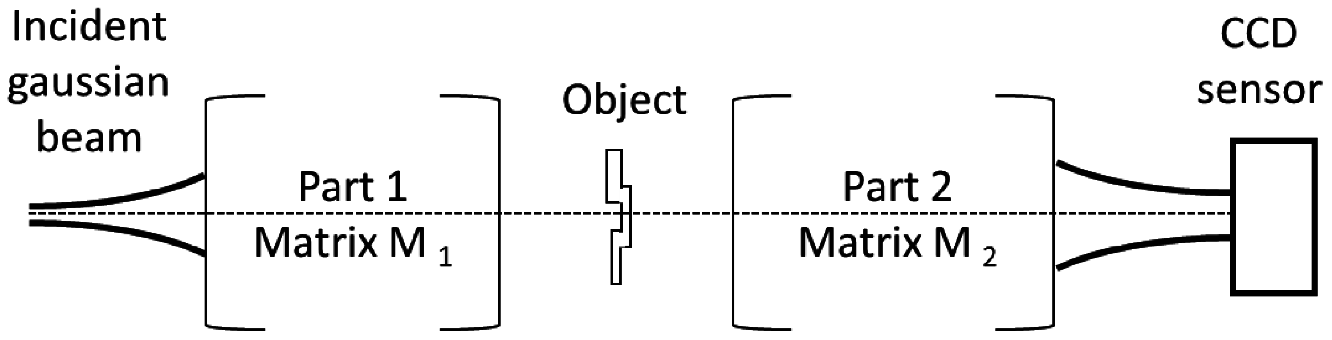
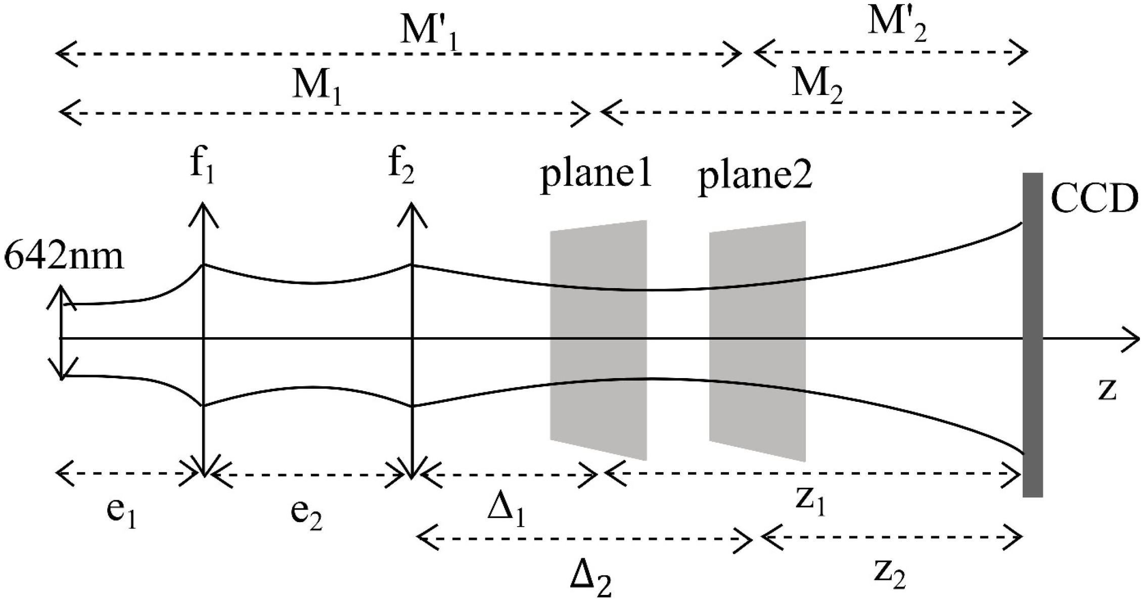
2. Numerical Simulator

2.1. Amplitude Distribution of the Beam in the Plane of the Object

The basic idea of Digital In-line Holography (DIH) is to record the intensity pattern diffracted by an object on an electronic array sensor. The object is then reconstructed numerically using image processing. Figure 1 is the typical set-up of a DIH experiment using an incident Gaussian beam. This specific case is well adapted to our experiments that use in most cases a single-mode laser beam.

Figure 1. Typical Digital In-Line Holography set-up.

Figure 1. Typical Digital In-Line Holography set-up.

Part 1 allows an appropriate illumination of the object. Part 2 is the “imaging” system (leading to a “transport” of the diffraction pattern from the object to the sensor). In order to interpret precisely the experimental results, it is necessary to develop a general numerical model that can describe any set-up. We present here the simulator that has been developed, using the scalar theory of diffraction. At the beginning of the propagation, the waist of the incident Gaussian beam is located at the origin (z = 0). z is the longitudinal axis of propagation (horizontal axis on Figure 1). In the next equations, the transverse axes will be noted µ and ν in the plane of the laser source, ξ and η in the plane of the particle, x and y in the plane of the CCD sensor. The electric field amplitude in the incident plane can be written as follows:

$$G\left(\mu ,\nu ,z=0\right)=G\left(\mu ,\nu \right)=\exp \left(-\frac{{\mu }^2+{\nu }^2}{{\omega }_0^2}\right)$$

(1)

where ω₀ is the waist of the beam. Then the laser beam propagates through the first optical system from the incident plane to the object plane. This part of the optical set-up is described by an optical transfer matrix M₁ as can be seen in Figure 1. The complex field amplitude of the wave in the plane of the object is noted G₁. It is obtained from a generalized Fresnel integral [19,25,26,27]. G₁ is given by:

$$\begin{array}{c}{G}_1(\xi ,\eta )=\frac{\exp \left(i\frac{2\pi }{\lambda }{\ell }_1\right)}{i\lambda \sqrt{B_1^x{B}_1^y}}{\displaystyle {\int }_{{ℝ}^2}G\left(\mu ,\nu \right)}\exp \left(i\frac{\pi }{\lambda B_1^x}\left[A_1^x{\mu }^2-2\xi \mu +D_1^x{\xi }^2\right]\right)\\ \exp \left(i\frac{\pi }{\lambda B_1^y}\left[A_1^y{\nu }^2-2\eta \nu +D_1^y{\eta }^2\right]\right)d\mu d\nu \end{array}$$

(2)

where ℓ₁ is the optical path between the incident plane and the object plane. $A_1^{x,y}$, $B_1^{x,y}$, and $D_1^{x,y}$ are the matrix elements of the matrix $M_1^{x,y}$, where $M_1^x=M_1^y=M_1$ for an axisymmetric system. $M_1^x$ and $M_1^y$ will be different for a cylindrical system. ξ and η are the transverse coordinates in the object plane. Substituting Equation (1) into Equation (2), the complex amplitude G₁(ξ, η) in the object plane becomes:

$$G_1(\xi ,\eta )=\frac{\exp \left(i\frac{2\pi }{\lambda }{\ell }_1\right)}{i\lambda \sqrt{B_1^x{B}_1^y}}{G}_0{K}_1^x{K}_1^y\exp \left[-\left(\frac{{\xi }^2}{{\omega }_{1_x}^2}+\frac{{\eta }^2}{{\omega }_{1_y}^2}\right)\right]\exp \left[-\frac{i\pi }{\lambda }\left(\frac{{\xi }^2}{R_{1x}}+\frac{{\eta }^2}{R_{1y}}\right)\right]$$

(3)

with $K_1^{x,y}={\left(\frac{\pi {\omega }_0^2}{1-i\frac{\pi {\omega }_0^2}{\lambda }\left(\frac{A_1^{x,y}}{B_1^{x,y}}\right)}\right)}^{1/2}$, ${\omega }_{1_{x,y}}=\left(\frac{\lambda B_1^{x,y}}{\pi \omega }\right){\left[1+{\left(\frac{\pi {\omega }_0^2}{\lambda }\frac{A_1^{x,y}}{B_1^{x,y}}\right)}^2\right]}^{1/2}$, $R_{1_{x,y}}=-\frac{B_1^{x,y}}{D_1^{x,y}-\frac{A_1^x{\left(\frac{\pi {\omega }_0^2}{\lambda B_1^{x,y}}\right)}^2}{1+{\left(\frac{\pi {\omega }_0^2}{\lambda }\frac{A_1^{x,y}}{B_1^{x,y}}\right)}^2}}$, where ω_1x,y and R_1x,y are respectively the beam waist radii and the beam curvatures in the object plane. They are deduced from the classical formula of Gaussian beams. It is important to note that this formulation allows the description of cylindrical systems, by separation of the two transfer matrices along both transverse axes : $M_1^x$ and $M_1^y$. The details of this calculus can be found in the appendix of reference [19].

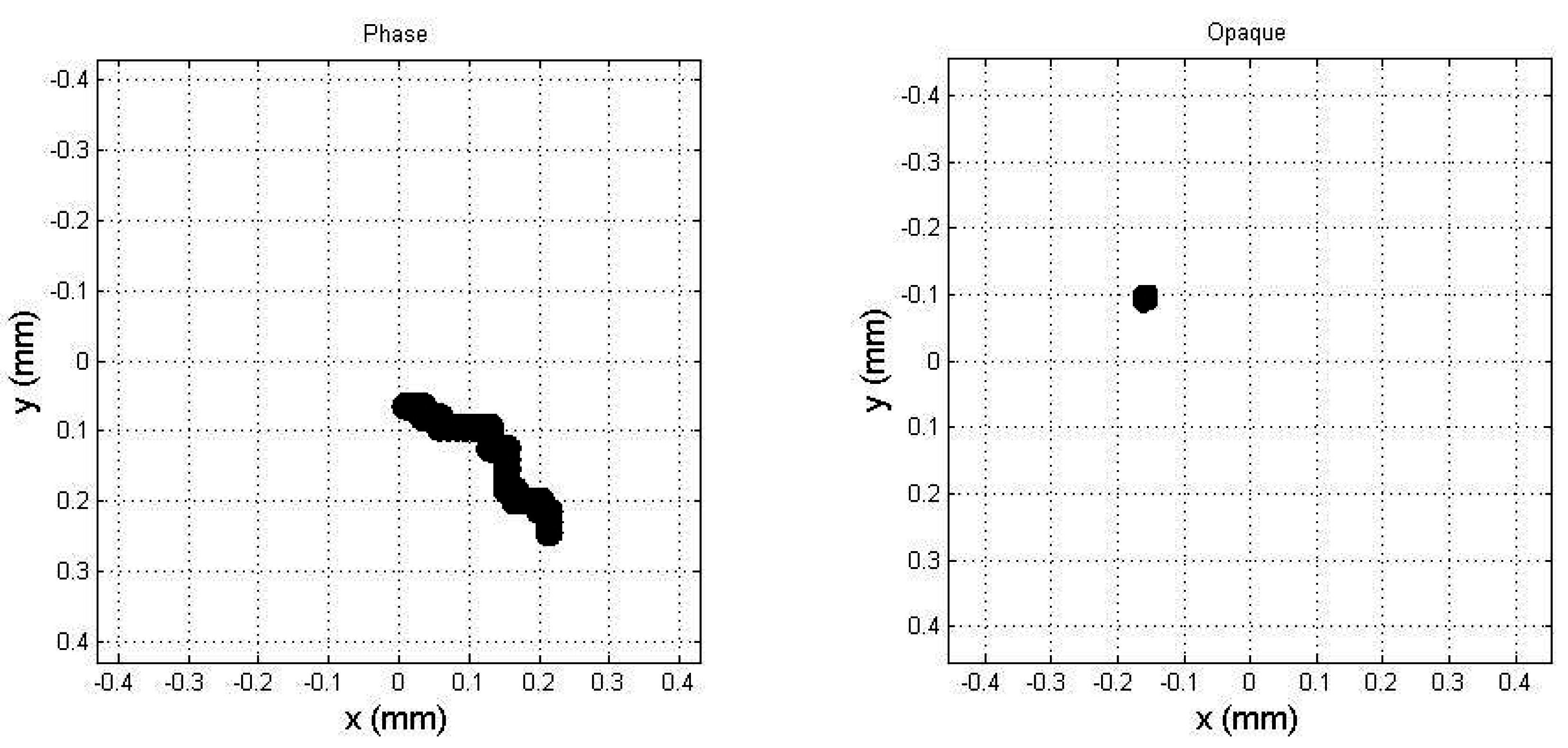
2.2. Definition of the Objects

In order to describe propagation of light through the second part of the system, it is then necessary to evaluate the transmission coefficient of the diffracting element. We have developed a library of opaque, semi-transparent or transparent phase objects. They are described by a transmission coefficient T (ξ, η). The objects are created from the collection of small circular disks. Both opaque and phase objects can be described. Opaque objects are defined by a collection of disks whose transmission coefficient is 0 inside the disk and 1 outside. For transparent objects, the transmission value inside the object is equal to e^iϕ and equal to 1 outside the object. The procedure is slightly longer. We realize a collection of circular opaque objects. The transmission coefficient of the object is then modified. We can further create an object where ϕ is not constant. For both opaque and phase objects, we can adjust the characteristic dimensions of the object. Some examples will be presented in the next sections.

2.3. Amplitude and Intensity Distributions in the Plane of the CCD Sensor

A second generalized Huygens-Fresnel transform gives the expression of the electric field in the CCD plane: G₂. It is given by the following relation:

$$\begin{array}{c}{G}_2(x,y)=\frac{\exp \left(i\frac{2\pi }{\lambda }{\ell }_2\right)}{i\lambda \sqrt{B_2^x{B}_2^y}}{\displaystyle {\int }_{{ℝ}^2}{G}_1}(\xi ,\eta )T(\xi ,\eta )\exp \left[i\frac{\pi }{\lambda B_2^x}\left(A_2^x{\xi }^2-2\xi x+D_2^x{x}^2\right)\right]\\ \exp \left[i\frac{\pi }{\lambda B_2^y}\left(A_2^y{\eta }^2-2\eta y+D_1^y{y}^2\right)\right]d\xi d\eta \end{array}$$

(4)

where ℓ₂ is the optical path between the object plane and the CCD plane. $A_2^{x,y}$, $B_2^{x,y}$, and $D_2^{x,y}$ are the coefficients of the matrices $M_2^{x,y}$ which describe the second part of the optical system (see Figure 1). We have $M_2^x=M_2^y=M_2$ for an axisymmetric system. T is the transmittance of the object. x and y are the transverse coordinates in the sensor plane. This second integral is evaluated numerically. The intensity distribution recorded by the CCD sensor is then obtained from:

$$I(x,y)=G_2(x,y)·\overline{G_2(x,y)}$$

(5)

where the overline refers to the complex conjugate.

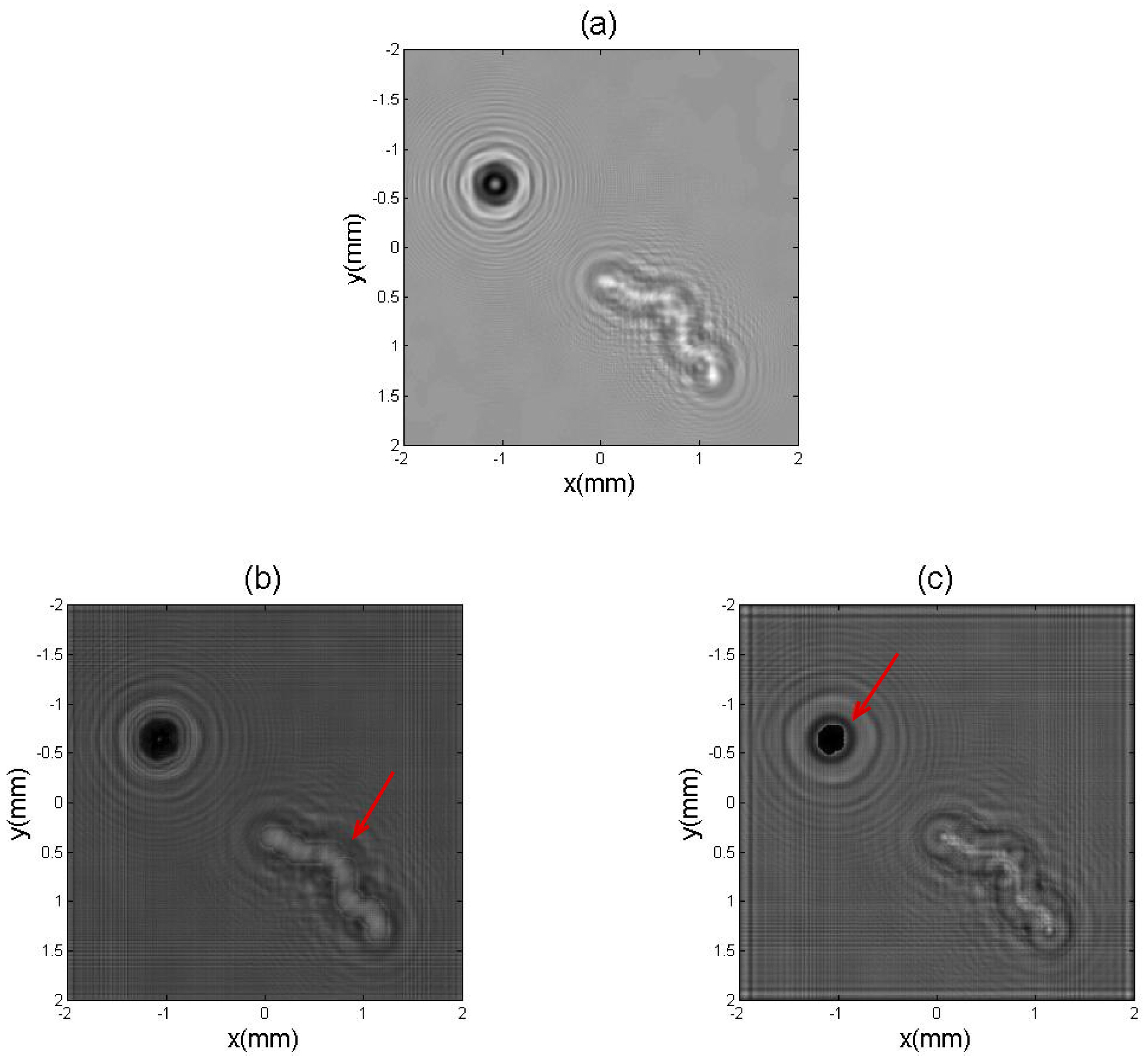
2.4. Hologram Analysis by Fractional Fourier Transform

The next step is the reconstruction of the objects from the holograms. Different tools can be used: wavelet transform, Fresnel transform. We use here the 2 Dimensional-FRactional-order Fourier Transform (2D-FRFT) [28,29,30,31]. The definition of the 2D-FRFT that we use is:

$${\mathcal{F}}_{{\alpha }_x,{\alpha }_y}\left[I\left(x,y\right)\right]\left(x_{\alpha },y_{\alpha }\right)={\displaystyle {\int }_{{ℝ}^2}{N}_{{\alpha }_x}}\left(x,x_{\alpha }\right)N_{{\alpha }_y}\left(y,y_{\alpha }\right)dx dy$$

(6)

with ${\alpha }_p=\frac{a_p\pi }{2}$ (p = x, y) and 0 ≤ |α_p| ≤ π/2. The kernel of the fractional operator is defined by:

$$N_{{\alpha }_p}(x,x_{\alpha })=C\left({\alpha }_p\right)\exp \left(i\pi \frac{x^2+x_{\alpha }^2}{s_p^2\tan {\alpha }_p}\right)\exp \left(-\frac{i2\pi x_{\alpha }x}{s_p^2\sin {\alpha }_p}\right)$$

(7)

with C (α_p) defined by:

$$C\left({\alpha }_p\right)=\frac{\exp \left(-i\left(\frac{\pi }{4}\mathrm{sign}(\sin {\alpha }_p)\right)-\frac{{\alpha }_p}{2}\right)}{{\left|s_p^2\sin {\alpha }_p\right|}^{1/2}}$$

(8)

Coefficient C(α_p) enables conservation of energy. Parameters s_p (p = x or y) are defined from the experimental set-up according to [32]:

$$s_p^2=N_p\cdot {\delta }_p^2$$

(9)

where Np are the numbers of pixels of the image along x or y axes, and the constants δ_p are the pixel sizes along both axes (p = x or y). In practice δ_x= δ_y. To reconstruct the image of the particle, we evaluate the 2D-FRFT of the diffraction pattern. The diffraction pattern contains a term with a linear chirp φ. This linear chirp is easily recovered through 2D-FRFT operation. The kernel of the 2D-FRFT operator is indeed composed of a linearly-chirped function, leading to applications in spatial optics when considering diffraction patterns (as here) or in temporal optics when considering chirped pulses [33]. The best reconstruction plane is reached when [19]:

φ_a ± φ = 0

(10)

where φ_a is the phase contained in 2D-FRFT and φ is the phase contained in the diffraction pattern. From this condition, the optimal fractional orders of reconstruction ${\alpha }_x^{opt}$ and ${\alpha }_y^{opt}$ can be obtained.

The existence of analytical relations that link optimal order of reconstruction to experimental parameters of a set-up are particularly interesting for different reasons: first, it allows 3D-localization of the particles under study, whatever the set-up is. In addition, it allows localization of defaults, present in the optical system, that create their own diffraction pattern on the sensor (which acts as noise). For example, we could localize the position of a scratch on a plexiglas cylinder. It was deduced from the analysis of the experimental hologram with these analytical relations. It was then confirmed experimentally watching the inner of the pipe once the set-up was uninstalled [23]. As a perspective, we think that our simulator combined to such analytical relations will allow to understand the sources of speckle noise that can alter the quality of holograms.

3. Simulation of Two Objects in Different Longitudinal Planes: Mixing of Opaque and Phase Objects

In this section, two irregular objects are generated in two different longitudinal planes. Each object has its own size and shape as shown in Figure 2. The object in plane 1 is a phase object (left of Figure 2) and the object in plane 2 is an opaque object (right of Figure 2). The numerical setup is presented in Figure 3. We evaluate separately the two diffraction patterns created by object 1 and by object 2 respectively. As both grids do not necessarily have the same pixel size (due to sampling conditions used when realizing both numerical Fresnel integrals), we use an interpolation function to super-impose both diffraction patterns. Noise can be added as well. As in [20], we assume that multiple scattering can be neglected (i.e., the part of the light diffracted by the first object and then by the second object).

Figure 2. Simulated phase particle (left) with phase shift φ = 0.3 π and opaque particle (right).

Figure 2. Simulated phase particle (left) with phase shift φ = 0.3 π and opaque particle (right).

The incident beam is a Gaussian beam. The initial beam waist is ω₀ = 2.3 µm. The wavelength is λ = 642 nm. The simulated configuration respects e₁ = 58.8 mm, f₁ = 42.8 mm, e₂ = 342.84 mm, f₂ = 5.5 mm. The first object is located at distance Δ₁ = 9.5 mm and the second object is located at distance Δ₂ = 10 mm from the second lens as described in Figure 3. The distance between the second lens and the CCD sensor equals 18 mm.

Figure 3. Simulated set-up.

Figure 3. Simulated set-up.

For the two objects, the system introduces magnification factors between the object plane and the CCD plane. They are given analytically by the following relation:

$$g_{1,2_{x,y}}=\frac{{\omega }_{to{t}_{x,y}}}{{\omega }_{1,2_{x,y}}}$$

(11)

where g_1,2x,y are the magnification factors between Plane 1 (or Plane 2) and the CCD plane. w_1,2x,y are the beam waist dimensions (along x and y, respectively) of the unperturbed Gaussian beam in Plane 1 (or in Plane 2 respectively). w_totx,y are the beam waist dimensions of the unperturbed Gaussian beam in the plane of the CCD sensor. They are given by:

$${\omega }_{to{t}_{x,y}}=\left(\frac{\lambda B_{tot}^{x,y}}{\pi {\omega }_0}\right){\left[1+{\left(A_{tot}^{x,y}\frac{\pi {\omega }_0^2}{\lambda B_{tot}^{x,y}}\right)}^2\right]}^{1/2}$$

(12)

$A_{tot}^p$ and $B_{tot}^p$ (with p = x or y) are the matrix elements of the transfer matrix describing the whole system between the laser source and the CCD sensor: $M_{tot}^p=M_2^p\times M_1^p$. In the simulation, the sensor size is 1024 × 1024 pixels and each pixel is 4.4 × 4.4 µm². The magnification factor introduced by the system for the object in Plane 1 is equal to 6.8, while it is equal to 5.3 for the object in plane 2.

Figure 4. (a) Simulated hologram considering both phase and opaque objects located in two different planes; (b) Reconstructed phase object with optimal order ${\alpha }_{x,y}^{opt}$ = −0:600 π/2 (red arrow); (c) Reconstructed opaque object with optimal order ${\alpha }_{x,y}^{opt}$ = −0:686 π/2 (red arrow).

Figure 4. (a) Simulated hologram considering both phase and opaque objects located in two different planes; (b) Reconstructed phase object with optimal order ${\alpha }_{x,y}^{opt}$ = −0:600 π/2 (red arrow); (c) Reconstructed opaque object with optimal order ${\alpha }_{x,y}^{opt}$ = −0:686 π/2 (red arrow).

Figure 4a is the hologram of the two objects recorded by the CCD sensor. Figure 4b,c show the optimal reconstruction of the two objects. For reconstruction of the objects, the 2D-FRFT is applied to the hologram. The optimal fractional orders for the objects in Figure 4b,c are –0.600 π/2 and –0.686 π/2, respectively. These two optimal fractional orders of the reconstructed objects give the correct longitudinal positions along z-axis of both objects. These reconstructions show the difference between opaque and phase objects: for the pure phase object in Figure 4b, a bright and a dark contour due to the discontinuity are observed at the edge of the object as mentioned in [13]. The intensity inside the reconstructed object can be higher than the continuous background. For the opaque object in Figure 4c, the intensity in the reconstructed object is zero. Moreover, the analysis of the patterns of the reconstructed objects leads to the size and the 2D-shape of the objects. As classically observed with in-line holography, the reconstructed objects are surrounded by fringes due to the twin image. They “scramble” the reconstruction. Nevertheless, the reconstruction remains possible and a quantitative analysis can be carried out from the reconstructed objects.

Figure 5. Transverse intensity profile of the reconstructed phase (a) and opaque (b) object: $\left|{\mathcal{F}}_{{\alpha }_x^{opt},{\alpha }_y^{opt}}\left[I\left(x,y\right)\right]\left(x_{\alpha },y_{\alpha }\right)\right|$.

Figure 5. Transverse intensity profile of the reconstructed phase (a) and opaque (b) object: $\left|{\mathcal{F}}_{{\alpha }_x^{opt},{\alpha }_y^{opt}}\left[I\left(x,y\right)\right]\left(x_{\alpha },y_{\alpha }\right)\right|$.

Intensity profiles of these phase and opaque reconstructed objects are plotted in Figure 5a,b, respectively. The size of the phase object can be estimated from the distance between both discontinuities which are indicated by two arrows in Figure 5a. For the opaque object, the width between both discontinuities of the intensity profile represents its size. From the intensity profile of the two objects and their magnification factors (5.3 and 6.8, for the phase and opaque objects, respectively), the real size of the phase object along x-axis is 24.8 µm and the real size of the opaque object along x-axis is 20.1 µm, respectively. Size measurements correspond to the original sizes of the two simulated objects in Figure 2. For different values of the phase shift introduced by the irregularly-shaped phase object, the transverse reconstructed intensity profiles for φ = 0.25 π, 0.5 π, and π are presented in Figure 6 (in solid line, dotted line and dashed line respectively). The curves have been plotted on the same figure. A continuous background has been added on these plots to separate them for clarity (it should be suppressed for a quantitative analysis). A reconstructed “phase jump” is clearly observed on the transverse profiles of Figure 6: it is the abrupt transition between points A and B (points plotted in the case φ = π). The amplitude of the discontinuity is directly linked to the phase shift introduced by the object. It has been shown that parameter $\frac{y_A-y_B}{y_c}$ is a monotonic function versus φ for a circular object [13]. y_A, y_B and y_c are normalized intensities measured on the three points A, B and C of the transverse profile defined in Figure 6. The present simulator allows to evaluate this parameter for any complex phase object. The method is efficient when 0.2 π < φ < 1.6 π. In other cases, the discontinuity is too small to be observed experimentally. Parameter φ can be recovered from estimated parameter $\frac{y_A-y_B}{y_c}$. A comparison of experimental results with simulation allows to validate the determination of the phase shift introduced by the object.

Figure 6. Transverse intensity profiles of the reconstructed phase objects $\left(\left|{\mathcal{F}}_{{\alpha }_x^{opt},{\alpha }_y^{opt}}\left[I\left(x,y\right)\right]\left(x_{\alpha },y_{\alpha }\right)\right|\right)$ when φ = 0.25 π (solid line), φ = 0.5 π (dotted line) and φ = π (dashed line).

Figure 6. Transverse intensity profiles of the reconstructed phase objects $\left(\left|{\mathcal{F}}_{{\alpha }_x^{opt},{\alpha }_y^{opt}}\left[I\left(x,y\right)\right]\left(x_{\alpha },y_{\alpha }\right)\right|\right)$ when φ = 0.25 π (solid line), φ = 0.5 π (dotted line) and φ = π (dashed line).

4. Two Examples of Application

4.1. Simulation of Phase Objects in a Droplet for Detection of Nanoparticles

We performed recently Digital In-line Holography experiments to reconstruct inclusions in a droplet [21,34]. In such experiments, the droplet itself induces a magnification factor which is added to the magnification introduced by the imaging system. Using our formalism, the two sides of the droplet and propagation through the droplet can be taken into account as effective optical elements by introduction of their own transfer matrices in the global optical transfer matrices M₁ and M₂. Let us consider the experimental set-up of Figure 7. The beam emitted by a fibered-laser diode is collimated using a first lens and then focused in the vicinity of a suspended water droplet with a microscope objective. Calibrated microspheres (diameter 20 µm) are introduced in the droplet. Figure 8 (on the left) shows optimal reconstruction of some of the microspheres. The wavelength of the incident beam is 642 nm. The diameter of the water droplet is 1.5 mm and its refractive index is 1.33. The other parameters are e₁ = 42.8 mm, f₁ = 42.8 mm, e₂ = 135.6 mm, f₂ = 5.5 mm, e₃ = 10 mm, z₁ = 0.825 mm, z₂ = 1.125 mm, and z = 9.7 mm. Let us now present in Figure 8 (on the right) the optimal reconstruction issued from a simulated hologram. In the case of this reconstruction, we have considered 7 circular particles: 4 are opaque objects, 3 are transparent phase objects (phase shift introduced π). The fact that the particles are located in a droplet is not a problem. The different optical elements of the droplet are considered through the appropriate definition of matrices M₁ and M₂. The different inclusions are clearly reconstructed. The opaque and non-opaque objects are easily identified. The possibility to simulate this experiment is particularly attractive for us. This set-up can indeed be used to detect 50 nm nanoparticles [22]: the droplet is seeded with nanoparticles. The droplet is then heated using a second laser (a frequency-doubled Nd:YAG laser emitting 4 ns, 10 mJ pulses in our case). Heating a nanoparticle creates a bubble which is reconstructed using Digital In-Line Holography [22]. For more details concerning the description of spherical micro-bubbles in this experiment, please refer to [22]. This indirect detection method is particularly efficient. With this new simulator that can describe arbitrarily-shaped phase objects as arbitrarily-shaped bubbles, we should be able to obtain information on morphology of nanoparticles through analysis of the shape of microbubbles in the future [35]. Our numerical model allows this.

Figure 7. Experimental set-up for the reconstruction of droplet’s inclusions.

Figure 7. Experimental set-up for the reconstruction of droplet’s inclusions.

Figure 8. (a) Experimental reconstruction of inclusions in a droplet; (b) Simulated reconstruction of opaque and transparent inclusions in a droplet.

Figure 8. (a) Experimental reconstruction of inclusions in a droplet; (b) Simulated reconstruction of opaque and transparent inclusions in a droplet.

4.2. Library of Ice Crystal Objects for the Calibration of Interferometric Airborne Instruments

We develop an airborne instrument to detect and characterize droplets and ice crystals in the atmosphere [36]. The technique used is interferometric particle imaging [37,38,39]. It has been chosen because fast algorithms can be developed that analyze directly a global image [36]. The instrument records on a CCD sensor the out-of-focus image of the scattering particle. In the case of droplets, the out-of-focus image shows regular interference fringes due to interference of both reflected and refracted beams. In the case of irregular rough particles such as ice crystals, the out-of-focus image shows a speckle-like pattern. The size of the droplet is deduced from the frequency of the fringes, while size and ellipticity of irregular particles are deduced from size and ellipticity of the speck of light in the speckle pattern [40]. In this last case, it can be demonstrated that the 2-Dimensional Fourier transform of the speckle pattern gives the 2-Dimensional autocorrelation of the global shape of the object [41]. The development of the airborne instrument requires its calibration in laboratory using a second well-known technique. Digital In-line Holography is perfectly appropriate. But the experimental set-up in laboratory requires experiments in cold chambers with different optics and windows. Our matrix-based numerical model allows to describe such environmental conditions by the appropriate definition of the correct optical transfer matrices. For future studies, we have developed a library of the most-common ice crystals that can be observed in the atmosphere. Some exemples are presented in Figure 9: a dendritic crystal with sector-like ends (top left) a malformed crystal (top right), an ordinary dendritic crystal (bottom left) and a crystal with sectorlike branches (bottom right).

Figure 9. Some examples from our library of transparent phase objects describing ice crystals. A dendritic crystal with sector-like ends (top left); A malformed crystal (top right); An ordinary dendritic crystal (bottom left) and a crystal with sectorlike branches (bottom right).

Figure 9. Some examples from our library of transparent phase objects describing ice crystals. A dendritic crystal with sector-like ends (top left); A malformed crystal (top right); An ordinary dendritic crystal (bottom left) and a crystal with sectorlike branches (bottom right).

Using our simulator, Figure 10 shows the digital in-line hologram generated by a transparent particle whose form is the one of a dendritic crystal with sector-like ends (left) and its optimal reconstruction using 2D-FRFT (right). As the object is not opaque, the exact form of the reconstructed can be affected by different effects as for example an intense central peak, or ambiguous limits in different parts of the reconstruction. We think that the models developed should allow a better interpretation of experiments and artifacts encountered in the reconstructions. With the definition of the object presented in the previous section, any kind of object shapes can be simulated. Objects can be opaque or phase objects. Any optical system can be considered by the choice of the appropriate transfer matrices.

Figure 10. Transparent phase particle whose form is the one of a dendritic crystal with sector-like ends (top); Example of Digital In-line Hologram generated by this particle (bottom left) and its optimal reconstruction using 2D-FRFT (bottom right).

Figure 10. Transparent phase particle whose form is the one of a dendritic crystal with sector-like ends (top); Example of Digital In-line Hologram generated by this particle (bottom left) and its optimal reconstruction using 2D-FRFT (bottom right).

5. Conclusions

We have developed a numerical simulator for digital in-line holography applications. In-line holograms of arbitrarily shaped and arbitrarily located 2D opaque or phase objects are calculated using generalized Huygens-Fresnel integrals. With this formalism, the optical set-up is described in terms of optical transfer matrices. A wide number of spherical or cylindrical lenses can thus be taken into account, which makes the simulator applicable for design and description of in situ experiments. Noise can be added as well, whose spatial frequency can be arbitrarily defined. We discuss future applications of this simulator for detection of nanoparticles in droplets or calibration of airborne instruments that detect and measure ice crystals in the atmosphere. Digital Holography has applications in a wide range of applied sciences from investigation of particles in flows in fluid mechanics, to visualization of cells in biology or medicine, phase contrast metrology. This numerical simulator should thus become a very powerful tool for analysis and simulation of experimental results in a wide range of optical configurations.

References

1. Schnars, U.; Jueptner, W.P. Direct recording of holograms by a CCD target and numerical reconstruction. Appl. Opt. 1994, 33, 179–181. [Google Scholar] [CrossRef] [PubMed]
2. Katz, J.; Sheng, J. Applications of Holography in Fluid Mechanics and Particle Dynamics. Ann. Rev. Fluid Mech. 2010, 42, 531–555. [Google Scholar] [CrossRef]
3. Buraga-Lefebvre, C.; Coetmellec, S.; Lebrun, D.; Ozkul, C. Application of wavelet transform to hologram analysis: three-dimensional location of particles. Opt. Las. Eng. 2000, 33, 409–421. [Google Scholar] [CrossRef]
4. Pan, G.; Meng, H. Digital holography of particle fields: reconstruction by use of complex amplitude. Appl. Opt. 2003, 42, 827–833. [Google Scholar] [CrossRef] [PubMed]
5. Denis, L.; Fournier, C.; Fournel, T.; Ducottet, C.; Jeulin, D. Direct extraction of the mean particle size from a digital hologram. Appl. Opt. 2006, 45, 944–952. [Google Scholar] [CrossRef] [PubMed]
6. Desse, J.M.; Picart, P.; Tankam, P. Digital three-color holographic interferometry for flow analysis. Opt. Express 2008, 16, 5471–5480. [Google Scholar] [CrossRef] [PubMed]
7. Verrier, N.; Remacha, C.; Brunel, M.; Lebrun, D.; Coetmellec, S. Micropipe flow visualization using digital in-line holographic microscopy. Opt. Express 2010, 18, 7807–7819. [Google Scholar] [CrossRef] [PubMed]
8. Kim, M.K. Wavelength-scanning digital interference holography for optical section imaging. Opt. Lett. 1999, 24, 1693–1695. [Google Scholar] [CrossRef] [PubMed]
9. Kim, M.K. Tomographic three-dimensional imaging of a biological specimen using wavelength-scanning digital interference holography. Opt. Exp. 2000, 7, 305–310. [Google Scholar] [CrossRef]
10. Garcia-Sucerquia, J.; Xu, W.; Jericho, M.H.; Kreuzer, H.J. Immersion digital in-line holographic microscopy. Opt. Lett. 2006, 31, 1211–1213. [Google Scholar] [CrossRef] [PubMed]
11. Cuche, E.; Marquet, P.; Depeursinge, C. Simultaneous amplitude-contrast and quantitative phase-contrast microscopy by numerical reconstruction of Fresnel off-axis holograms. Appl. Opt. 1999, 38, 6994–7001. [Google Scholar] [CrossRef] [PubMed]
12. Cuche, E.; Bevilacqua, F.; Depeursinge, C. Digital holography for quantitative phase-contrast imaging. Opt. Lett. 1999, 24, 291–293. [Google Scholar] [CrossRef] [PubMed]
13. Brunel, M.; Coetmellec, S.; Lebrun, D.; Ait Ameur, K. Digital phase contrast with the fractional Fourier transform. Appl. Opt. 2009, 48, 579–583. [Google Scholar] [CrossRef] [PubMed]
14. Absil, E.; Tessier, G.; Gross, M.; Atlan, M.; Warnasooriya, N.; Suck, S.; Coppey-Moisan, M.; Fournier, D. Photothermal heterodyne holography of gold nanoparticles. Opt. Express 2010, 18, 780–786. [Google Scholar] [CrossRef] [PubMed]
15. Picart, P.; Leval, J. General theoretical formulation of image formation in digital Fresnel holography. J. Opt. Soc. Am. A 2008, 25, 1744–1761. [Google Scholar] [CrossRef]
16. Dubois, F.; Schockaert, C.; Callens, N.; Yourrassowsky, C. Focus plane detection criteria in digital holography microscopy by amplitude analysis. Opt. Express 2006, 14, 5895–5908. [Google Scholar] [CrossRef] [PubMed]
17. Atlan, M.; Gross, M.; Absil, E. Accurate phase-shifting digital interferometry. Opt. Lett. 2007, 32, 1456–1458. [Google Scholar] [CrossRef] [PubMed]
18. Gross, M.; Atlan, M. Digital holography with ultimate sensitivity. Opt. Lett. 2007, 32, 909–911. [Google Scholar] [CrossRef] [PubMed]
19. Verrier, N.; Coetmellec, S.; Brunel, M.; Lebrun, D. Digital in-line holography in thick optical systems: Application to visualization in pipes. Appl. Opt. 2008, 47, 4147–4157. [Google Scholar] [CrossRef] [PubMed]
20. Wu, X.; Meunier-Guttin-Cluzel, S.; Wu, Y.; Saengkaew, S.; Lebrun, D.; Brunel, M.; Chen, L.; Coetmellec, S.; Cen, K.; Grehan, G. Holography and micro-holography of droplets: A numerical standard. Opt. Commun. 2012, 285, 3013–3020. [Google Scholar] [CrossRef]
21. Coetmellec, S.; Wichitwong, W.; Grehan, G.; Lebrun, D.; Brunel, M.; Janssen, A.J.E.M. Digital in-line holography assessment for general phase and opaque particle. J. Eur. Opt. Soc. Rap. Publ. 2014, 9, 14021. [Google Scholar] [CrossRef]
22. Coetmellec, S.; Pejchang, D.; Allano, D.; Grehan, G.; Lebrun, D.; Brunel, M.; Janssen, A.J.E.M. Digital in-line holography in a droplet with cavitation air bubbles. J. Eur. Opt. Soc. Rap. Publ. 2014, 9, 14056. [Google Scholar] [CrossRef]
23. Brunel, M.; Shen, H.; Coetmellec, S.; Lebrun, D. Extended ABCD matrix formalism for the description of femtosecond diffraction patterns; application to femtosecond Digital In-line Holography with anamorphic optical systems. Appl. Opt. 2012, 51, 1137–1148. [Google Scholar] [CrossRef] [PubMed]
24. Brunel, M.; Shen, H.; Coetmellec, S.; Lebrun, D.; Ait Ameur, K. Phase contrast metrology using digital in-line holography: General models and reconstruction of phase discontinuities. J. Quant. Spectrosc. Radiat. Transf. 2013, 126, 113–121. [Google Scholar] [CrossRef]
25. Palma, C.; Bagini, V. Extension of the Fresnel transform to ABCD systems. J. Opt. Soc. Am. A 1997, 14, 1774–1779. [Google Scholar] [CrossRef]
26. Lambert, A.J.; Fraser, D. Linear systems approach to simulation of optical diffraction. Appl. Opt. 1998, 37, 7933–7939. [Google Scholar] [CrossRef] [PubMed]
27. Yura, H.T.; Hanson, S.G. Optical beam wave propagation through complex optical systems. J. Opt. Soc. Am. A 1987, 4, 1931–1948. [Google Scholar] [CrossRef]
28. McBride, A.C.; Kerr, F.H. On Namias fractional Fourier transforms. IMA J. Appl. Math. 1987, 39, 159–175. [Google Scholar] [CrossRef]
29. Namias, V. The fractional order Fourier transform and its application to quantum mechanics. J. Inst. Math. Its Appl. 1980, 25, 241–265. [Google Scholar] [CrossRef]
30. Lohmann, A.W. Image rotation, Wigner rotation, and the fractional Fourier transform. J. Opt. Soc. Am. A 1993, 10, 2180–2186. [Google Scholar] [CrossRef]
31. Coetmellec, S.; Lebrun, D.; Ozkul, C. Application of the two-dimensional fractional-order Fourier transformation to particle field digital holography. J. Opt. Soc. Am. A 2002, 19, 1537–1546. [Google Scholar] [CrossRef]
32. Mas, D.; Pérez, J.; Hernández, C.; Vázquez, C.; Miret, J.J.; Illueca, C. Fast numerical calculation of Fresnel patterns in convergent systems. Opt. Commun. 2003, 227, 245–258. [Google Scholar] [CrossRef]
33. Brunel, M.; Coetmellec, S.; Lelek, M.; Louradour, F. Fractional-order Fourier analysis for ultrashort pulse characterization. J. Opt. Soc. Am. A 2007, 24, 1641–1646. [Google Scholar] [CrossRef]
34. Wichitwong, W.; Coetmellec, S.; Lebrun, D.; Allan, D.; Grehan, G.; Brunel, M. Long exposure time Digital In-line Holography for the trajectography of micronic particles within a suspended millimetric droplet. Opt. Commun. 2014, 326, 160–165. [Google Scholar] [CrossRef]
35. Chaari, A.; Grosges, T.; Giraud-Moreau, L.; Barchiesi, D. Nanobubble evolution around nanowire in liquid. Opt. Express 2013, 21, 26942–26954. [Google Scholar] [CrossRef] [PubMed]
36. Querel, A.; Lemaitre, P.; Brunel, M.; Porcheron, E.; Grehan, G. Real-time global interferometric laser imaging for the droplet sizing (ILIDS) algorithm for airborne research. Meas. Sci. Technol. 2010, 21, 015306. [Google Scholar] [CrossRef]
37. Glover, A.R.; Skippon, S.M.; Boyle, R.D. Interferometric laser imaging for droplet sizing: A method for droplet-size measurement in sparse spray systems. Appl. Opt. 1995, 34, 8409–8421. [Google Scholar] [CrossRef] [PubMed]
38. Damaschke, N.; Nobach, H.; Tropea, C. Optical limits of particle concentration for multi-dimensional particle sizing techniques in fluid mechanics. Exp. Fluids 2002, 32, 143–152. [Google Scholar]
39. Shen, H.; Coetmellec, S.; Grehan, G.; Brunel, M. ILIDS revisited: elaboration of transfer matrix models for the description of complete systems. Appl. Opt. 2012, 51, 5357–5368. [Google Scholar] [CrossRef] [PubMed]
40. Brunel, M.; Coetmellec, S.; Grehan, G.; Shen, H. Interferometric out-of-focus imaging simulator for irregular rough particles. J. Eur. Opt. Soc. Rap. Publ. 2014, 9, 14008. [Google Scholar] [CrossRef]
41. Brunel, M.; Gonzalez Ruiz, S.; Jacquot, J.; van Beeck, J. On the morphology of irregular rough particles from the analysis of speckle-like interferometric out-of-focus images. Opt. Commun. 2015, 338, 193–198. [Google Scholar] [CrossRef]