Pipeline Damage Identification Based on Additional Virtual Masses

Institute of Intelligent Structural Systems, School of Civil Engineering, Dalian University of Technology, Dalian 116024, China
*
Author to whom correspondence should be addressed.
Appl. Sci. 2017, 7(10), 1040; https://doi.org/10.3390/app7101040
Submission received: 26 August 2017
/
Revised: 25 September 2017
/
Accepted: 1 October 2017
/
Published: 11 October 2017
Abstract
:To improve the identification sensitivity of local damages in pipelines, we propose an added virtual mass method thatprevents adding real masses to the pipeline. First, we develop a method of adding virtual masses to pipelines based on the virtual distortion method (VDM). Second, a frequency response to the added mass is constructed using the excitation and acceleration responses. The quantity of mass and the corresponding selected natural frequency with high sensitivity are both determined by the analyzing the sensitivity of the relationship between mass and natural frequency. Finally, the degree of damage can be accurately identified by adding virtual masses on the substructure of the pipeline combined with sensitivity and frequency. Using numerical simulations and experiments, we verify the feasibility of the added virtual mass method for the identification of damages to pipeline structures.
1. Introduction
Pipelines usually transport flammable, explosive, toxic, or corrosive media under extremely harsh environments. Therefore, long-term operation is prone to leakage or even explosion and other accidents [1]. For this reason, implementing effective structure health monitoring (SHM) for pipelines is very important, because damage identification provides a reliable theoretical basis for the detection, early warning, and safety assessment of such structures.
Currently, pipeline health monitoring is mainly carried out by assessing the integrity of the pipeline structure, which can help in detecting various damages, occurrence, and location and in identifying the degree of damage detected. Non-destructive testing techniques, such as radiation, electromagnetism, ultrasonic guided wave, acoustic emission, and modal method, are commonly used in pipeline damage detection. Among the aforementioned methods, only the vibration model detection method is relatively simple and easy to operate, which can be utilized under environment excitation. Therefore, damage identification based on modal information is widely used in pipeline damage. Li et al. [2] discussed a nondestructive testing technique based on the perturbation principle, in which a square change of frequency is applied to damage identification of pressure pipelines. Pandey [3] first proposed the application of the curvature mode in damage identification. Through finite element analysis, this author studied the relationship between curvature mode and damage. Hao et al. [4] located pipeline damage based on a curvature modal difference. Ren et al. [5] expressed strain as a function of displacement vibration mode and used the index of the strain modal difference rate to study damage location. Modal information is the basic parameter of a structure and does not change with the incentive. However, only several low natural frequencies are estimated because obtaining higher natural frequencies is difficult [6]. The amount of unknown parameters also becomes larger due to the complexity of structures. Hence, accurately identifying damages in the field of civil engineering is challenging. F, Khan et al. [7] discussed the implementation and validation of an integrated structural health monitoring (ISHM). The proposed ISHM scheme used three methods: digital image correlation (DIC), acoustic emission (AE) and guided ultrasonic waves (GUW).
In terms of the current research situation, the damage identification method based on structural vibration characteristics mainly includes: the method based on structural dynamic characteristics (frequency, vibration mode, flexibility matrix, strain mode, and so on), method based on frequency response (FRF), time series method, method based on model correction, Intelligent optimization algorithm, method based on probability and statistics and the method based on damage location vector (DLV).
Adding control parameters, such as mass and stiffness, on the structure provides an effective method for damage identification by changing the shape of the structure [8,9,10]. Increasing the amount of the modified structure is a good way to obtain a large number of data. However, adding mass or stiffness on structures in certain special situations is difficult. Therefore, the current paper presents a damage identification method using additional virtual masses based on the virtual distortion method (VDM). The proposed method is a rapid structural reanalysis method that employs virtual distortions or forces to simulate structural modification [11]. Via VDM, ample modified structure frequency responses are obtained. Hence, the extent of the damage to the original structure can be accurately estimated using the data from the original and virtual structures. The method is also used for the identification of structural parameters, such as stiffness, mass, moving mass, and damping [12,13,14,15].
Using the basic concept of VDM, this paper proposes the addition of virtual masses to pipeline structures and accurately identifying damage degree with combined sensitivity and frequency. We posit that doing so evades the difficulty of attaching real masses. The method divides a pipeline structure into several substructures and increases the sensitivity of the frequency to damage by adding virtual masses to each substructure. Constructing a response after adding virtual mass is key to this method, and frequency response by adding random mass can be obtained according to the measured force and acceleration frequency responses. First, this paper introduces the basic principle of damage identification based on additional VMD. Then, numerical simulation and experimental verification are carried out on the pipeline structure, which expands the applicability of the method in different structures. In this experiment, to quantify the degree of damage in the pipeline, a certain size of the hole is made to simulate the damage. The damage represents the longitudinal split of the pipe in real life, but in order to achieve the experimental results, the simulated damage is relatively large.
2. Damage Identification Method Based on Additional Virtual Masses
2.1. Additional Virtual Mass
After adding masses on a structure, frequency response can be calculated using the excitation and acceleration responses of the original structure. Hence, a new virtual structure can be created. The theoretical derivation process is as follows [16].
Assume that is the unit excitation applied to the p-degree of freedom (DOF) on the original structure and l is the acceleration frequency response function. If a certain mass is added and in the same direction as that of the p DOF, excitation is applied, then acceleration frequency response is . Hence, additional mass m only produces inertial force in the direction of p DOF, as . According to the basic concept of VDM, frequency response with additional mass m in the p DOF can be expressed as the sum of frequency response of the original structure and the response generated by mass inertia force .
In the equations above,
The variable is the excitation time in the p DOF, is the acceleration response, and represents the Fourier transform. Substituting Equation (3) into Equation (2) gives
Equation (4) shows that only by measuring excitation and acceleration response can we calculate the acceleration frequency response of structures with any added virtual mass m. In other words, where the acceleration sensor is arranged, virtual masses can be added. The method is easy to operate and the calculation is simple.
2.2. Damage Identification Based on Sensitivity
Assume that the global structure consists of n components, each defined as a substructure. Let the structural damage be modeled in terms of stiffness reduction ratios of the substructures. If the damage factor of the ith substructure is defined as , then . is the original undamaged stiffness matrix of the ith substructure expressed in the global DOFs. Hence, the global stiffness matrix of the damaged structure is assembled as
By adding a virtual mass to the real structure, the dynamic characteristics of the resulting virtual structure are changed compared with the original real structure . In this manner, the virtual structure can be designed and purposely used for damage identification. Here, the virtual mass is added to increase the relative sensitivity of natural frequencies with respect to damage parameter .
Assuming the damage vector , the characteristics of the kth natural frequency of the corresponding virtual structure (symbolically denoted by ) depend on three parameters: order k of natural frequency, virtual mass m, and its placement i. The virtual mass does not affect stiffness, and as such, the stiffness matrix of such a virtual structure is still . Let denote the absolute sensitivity of with respect to the extent of damage of the lth substructure
where is the kth mass-normalized global mode shape of the virtual structure .
According to the definition of sensitivity, if is the initial value of the damage factor, then a first-order approximation occurs between changes in the damage factor and structure frequency
We collect all frequencies in all structures , where , . Then, formula (7) is arranged as in the following sequence:
where
Damage factor can be approximated by Equation (10), which can be the initial value in the next iteration. Then, the new sensitivity matrix is constructed, and the above steps are repeated until it converges.
In the equation above, denotes the generalized inverse matrix of , which can be calculated by a singular value decomposition.
3. Numerical Simulation
A pipe structure model with fixed bearings at both ends is used to verify whether virtual masses can be used to increase the sensitivities of natural frequencies to local damages, as well as to illustrate the application principles of the proposed approach.
3.1. Finite Element Modeling
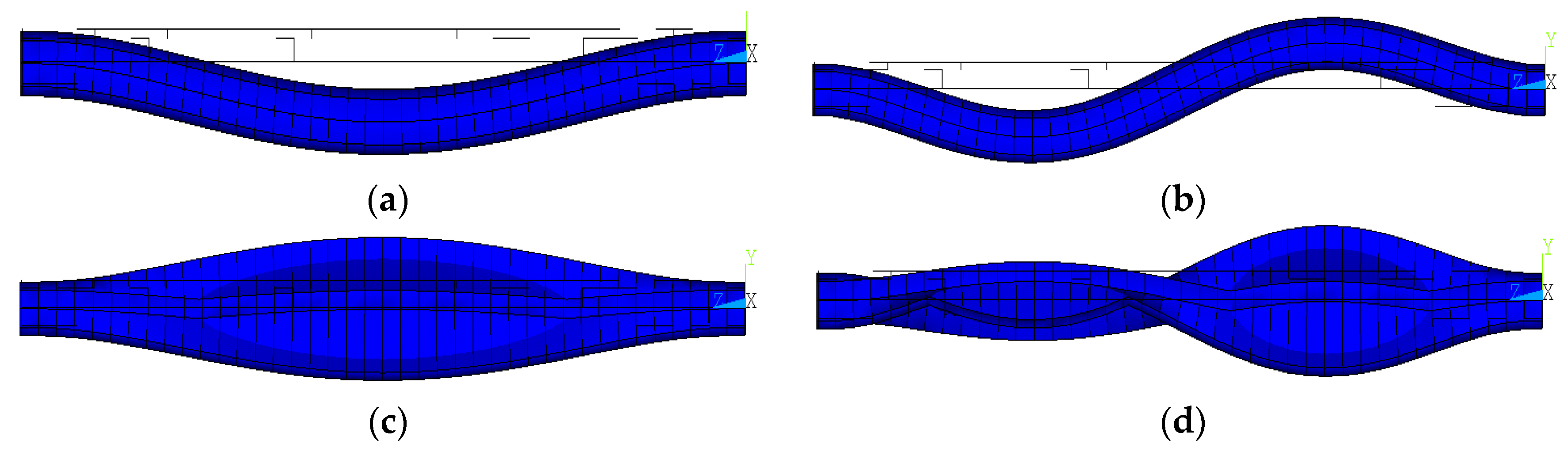
Modeling and analysis were carried out with ANSYS (15.0; ANSYS, Inc., Pittsburgh, PA, USA; 2013). Table 1 shows the pipeline parameters studied in this paper. The pipeline model uses shell63 element and both ends are fixed constraints. A total of 40 units are divided along the length and 8 units along the pipeline circumference. The pipeline is divided into 10 substructures along the axial direction and each substructure contains 32 units. The substructures are numbered as illustrated in Figure 1. Table 2 shows the first four natural frequencies of the pipe model. Figure 2a–d show the corresponding first four mode shapes. In the vibration pattern, the simple beam-type mode shapes give a low-order mode performance, whereas the torsion of the pipe gives a high-order mode of performance.
A shell63 element has 4 nodes and 6 DOFs (degrees of freedom). The initial finite element model is established with a total of 328 nodes and 1776 DOFs. Considering the actual engineering and for easy calculation, the Guyan method [17] was adopted to reserve the DOFs in the (x,y) direction and reduce all remaining DOFs. Finally, the DOFs of the pipeline model was reduced to 296. Table 3 shows the frequencies calculated from the “new model.”
3.2. Sensitivity Analysis with Virtual Masses
By adding mass m to the middle of the 10 substructures, the new structure is defined as virtual structure , (i = 1, 2, 3 … 10). Figure 3 depicts the results of the first four frequencies with the relative sensitivity of substructure i. Relative sensitivity is defined as
and is the result of sensitivity to the normalization of frequency, which is beneficial to the comparison and analysis.
Figure 3 shows that relative sensitivity varies for every pair of mass and sub-structure due to the symmetry of the pipeline constraints. Figure 3a shows the relative sensitivity cure for substructure 1/2/9/10. In the figure, we see that the relative sensitivity of the first and third frequencies increases with the mass. However, the relative sensitivity of the third frequency rises sharply from the initial stage to the peak, whereas the first rises and falls relatively gently with a peak of 7 kg. The relative sensitivity of the second frequency increases slowly with the additional mass. The fourth remained constant from the beginning to the lowest.
In combination with the above analysis and considering the ideal mode of the pipeline that can be obtained by the subsequent test, two virtual structures can be selected for the substructure near the bearing: one is the first frequency corresponding to , and the other is the second frequency corresponding to . In selecting additional mass value, the mass should be as small as possible to avoid impact on the structure itself and to ensure the improvement of relative sensitivity. Therefore, according to the sensitivity curve in Figure 3a, combined with the above analysis, the first frequency is selected as the modal information for the subsequent damage identification for substructure 1/2/9/10. The selected additional virtual mass () is 7 kg.
3.3. Excitation and Frequency Response
3.3.1. Frequency Response of the Original Model
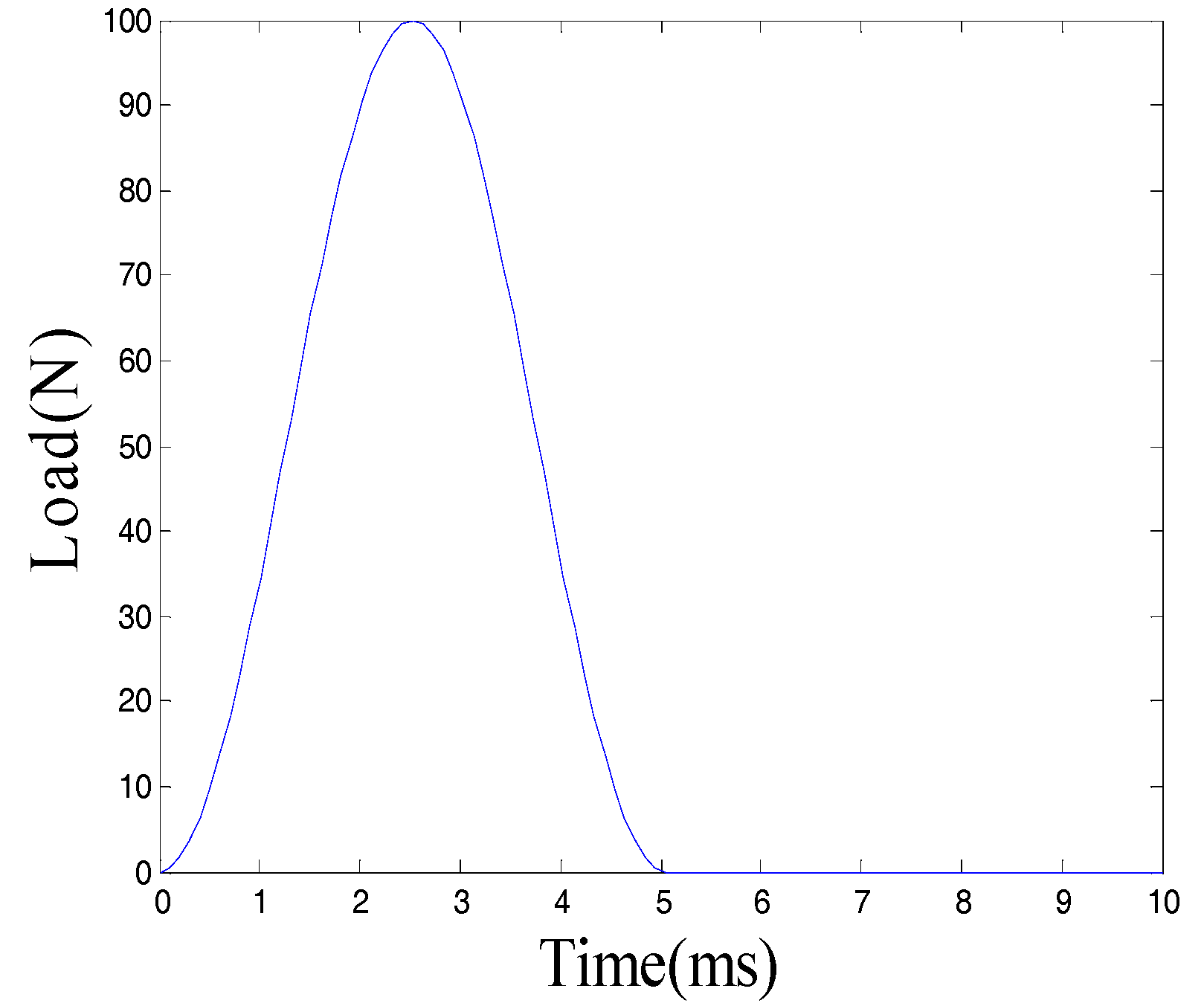
Figure 4 depicts a simulated hammer excitation applied in the middle of substructure 5. The sampling frequency was 10 kHz and a time interval of 2 s was considered. The simulated excitation lasted 5 ms and modeled the impact of a modal hammer (see Figure 4). To simulate real application, 5% Gaussian white noise was added to the excitation and response. To eliminate noise effectively, the wavelet de-noising method is used, and the selected wavelet basis is db8.Excitation without noise was applied to the structure, after which the structural responses were computed via the FE modelof the undamaged structure. Figure 5 shows the simulated measured acceleration response of the middle substructure along the vertical direction. Figure 6 depicts the frequency response after Fast Fourier Transform (FFT), where we extract the peak corresponding to the first three frequencies calculated via FE model (Section 3.1).
3.3.2. Frequency Response with Virtual Masses
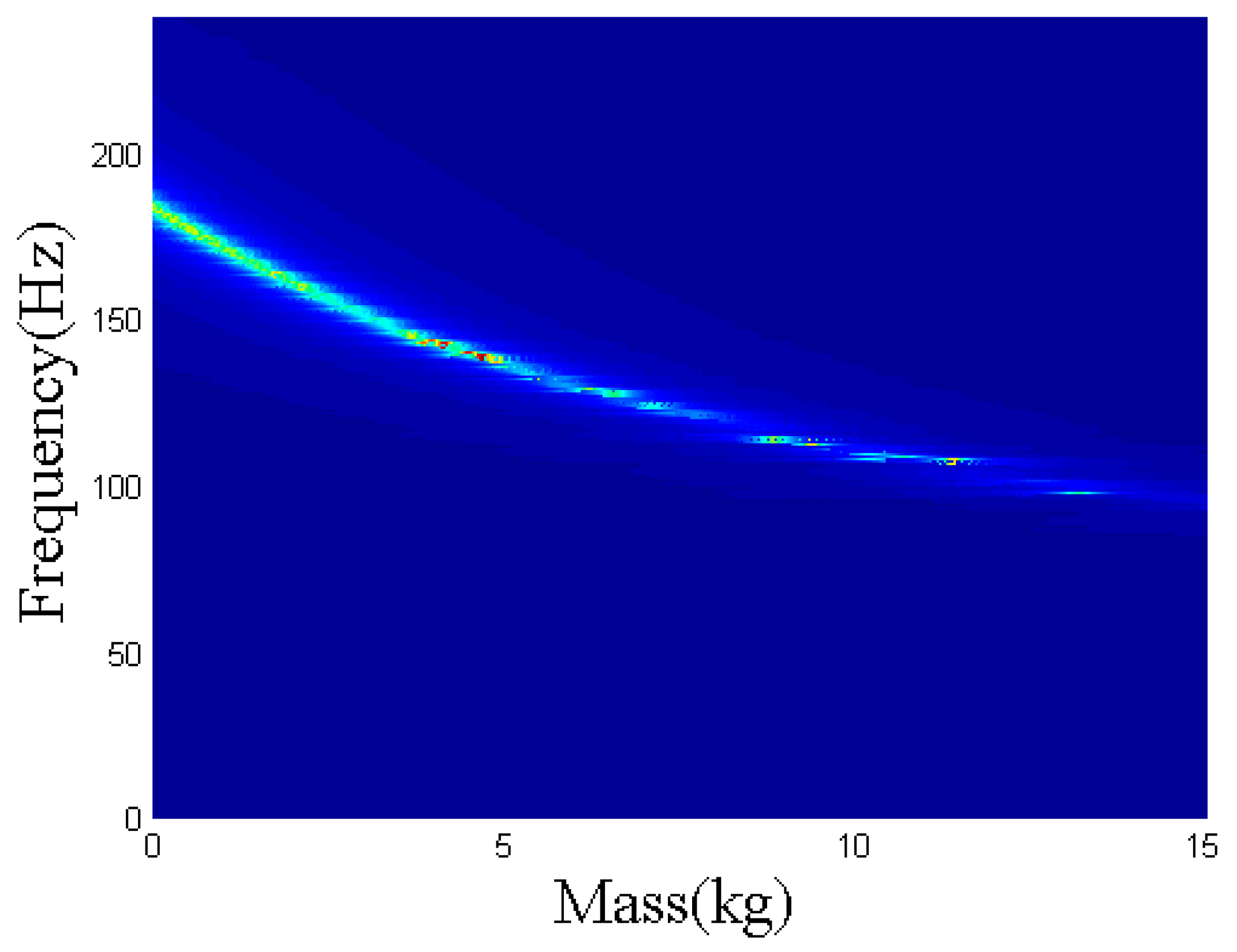
To construct the frequency response of the virtual structure with additional virtual masses, FT (Fourier Transform) with exponential window was performed on the noisy simulated measured excitation and responses. The result is used in Equation (4) to obtain the frequency response of the virtual structure G5 for the virtual mass kg. Figure 7 shows the nephogram of the constructed frequency response with respect to the virtual mass. As the mass increases, the first natural frequency decreases. Figure 8 illustrates the changes of the first frequency response after adding 0–8 kg in the middle of the substructure, which are directly calculated by using the frequency with different masses (FEM). Figure 9 shows the change of the first frequency with different masses by substituting the original frequency response into Formula (4). By comparing Figure 8 and Figure 9, we can say that the two are basically identical. Such a case indicates that the frequency response is effective and accurate after constructing additional virtual masses using VDM and does not need to reload the FEM, thereby greatly improving the computational efficiency.
3.4. Damage Identification
Using theoretical FEM, we multiply the stiffness Ki of several substructures using the theoretical damage vector μ to simulate the actual damage. In this section, damage identification is carried out in two kinds of conditions: single and multiple damages. Case 1 is that of damage occurring in substructure 5 with , whereas case 2 reflects the multiple damage that occurs on substructures 3, 4, and 7. Table 6 presents the specific damage vectors μ.
Figure 10 compares the selected natural frequencies. The figure shows that the change of the first frequency after damage is small with a 5 Hz reduction. The damage can be initially judged. In comparison, by attaching to the corresponding virtual masses, the frequency is significantly reduced at 112 Hz.
In the theoretical damage model, the excitation shown in Figure 4 is applied to the intermediate position of 10 substructures and their acceleration responses at the corresponding excitation position are calculated. Placing excitation and response while considering 5% noise in Equation (4), the frequency corresponding to the respective optimal virtual masses was constructed. Then, the frequency changes before and after the damage were combined with the sensitivity matrix of Formula (9), which was dominant and convergent. Hence, the damage factor of the simulation was iterated in Formula (10).
Figure 11 shows the single damage identification of substructure 5, and Figure 12 shows the multiple damage identification of the substructure 3/5/7. From the result of the numerical simulation, we conclude that damage identification of the substructure can be effectively realized by adding the virtual masses to the substructure and using the sensitivity matrix iteration.
4. Test of the Pipeline Damage Identification
4.1. Test Model
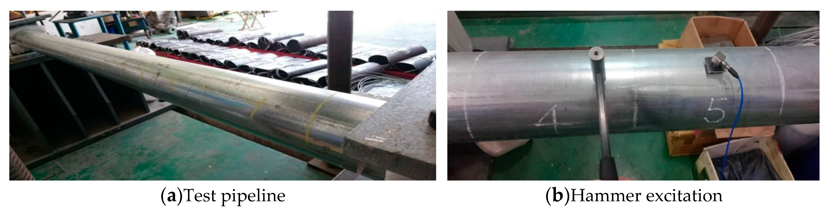
Figure 13 and Figure 14 present the test model of the pipeline structure. The pipeline steel used in this test is Q235, with 2 m in length and 3 mm thickness. Both ends are clamped to simulate fixed support. The net length after deducting the support is 1.9 m. The pipe is divided into 10 substructures with 9 nodes along the length, each of which is 200 mm long.
The nine nodes were selected as the hammer excitation points and node 5 was set as the pick-up point of the acceleration response. The piezoelectric acceleration sensor (sensitivity: 992 mV/g) was fixed to the upper surface of the pipeline with a small piece of magnet with a measured sampling frequency of 10 kHz. The experimental data were obtained according to the model and method. The results analyzed using Matlab software (R2014a; MathWorks, Inc, Natick, MA, USA; 2014) are shown below.
Figure 15 shows the measured excitation and acceleration response. Figure 16 presents the frequency response obtained by the FFT of the acceleration response, which is shown as the average of the multiple frequency responses. In the same figure, we can also see the first two vertical modes of the pipeline. Table 7 lists the specific frequencies consistent with the calculated frequencies. Such a case indicates the good reflection of the actual structure, which can be used as a benchmark for subsequent damage identification.
4.2. Damage Degree Identification
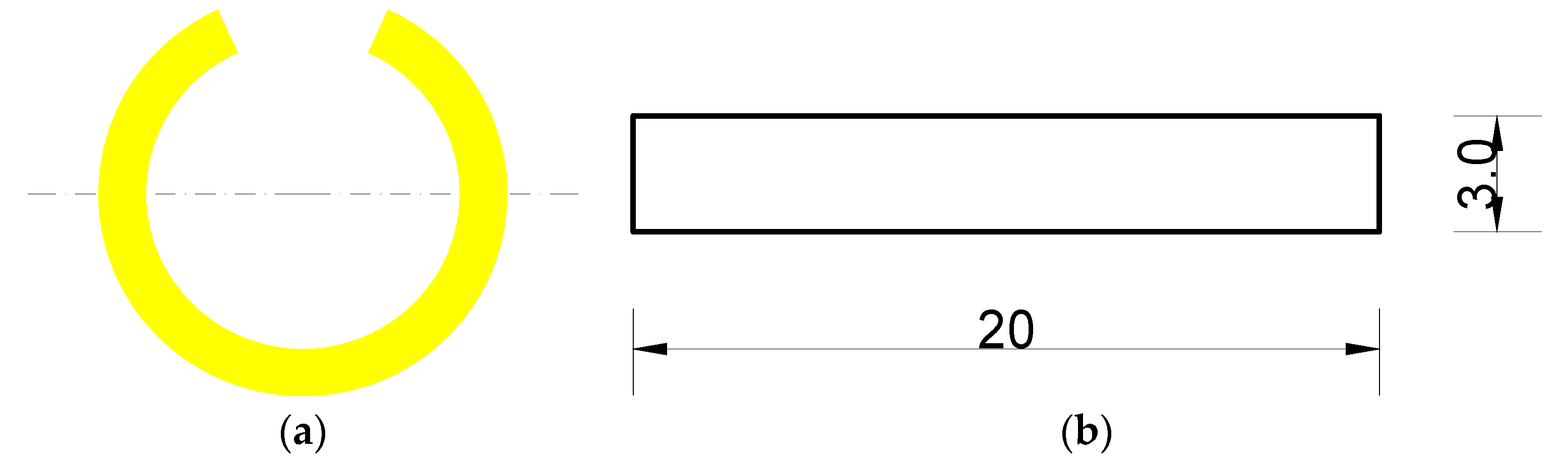
To verify the application effect of the method in the actual pipeline structure, the damage degree of substructure 5 was identified based on the laboratory pipeline model. A hole was dug inside substructure 5 to simulate damage. Figure 17a,b show the cross-section and size of the hole. The damage degree can be calculated using the material mechanics formula. As elastic modulus E is constant, the damage of stiffness EI is a reduction of the moment of inertia I. The calculated moment of inertia of the cross-section is reduced to 0.83 [18].
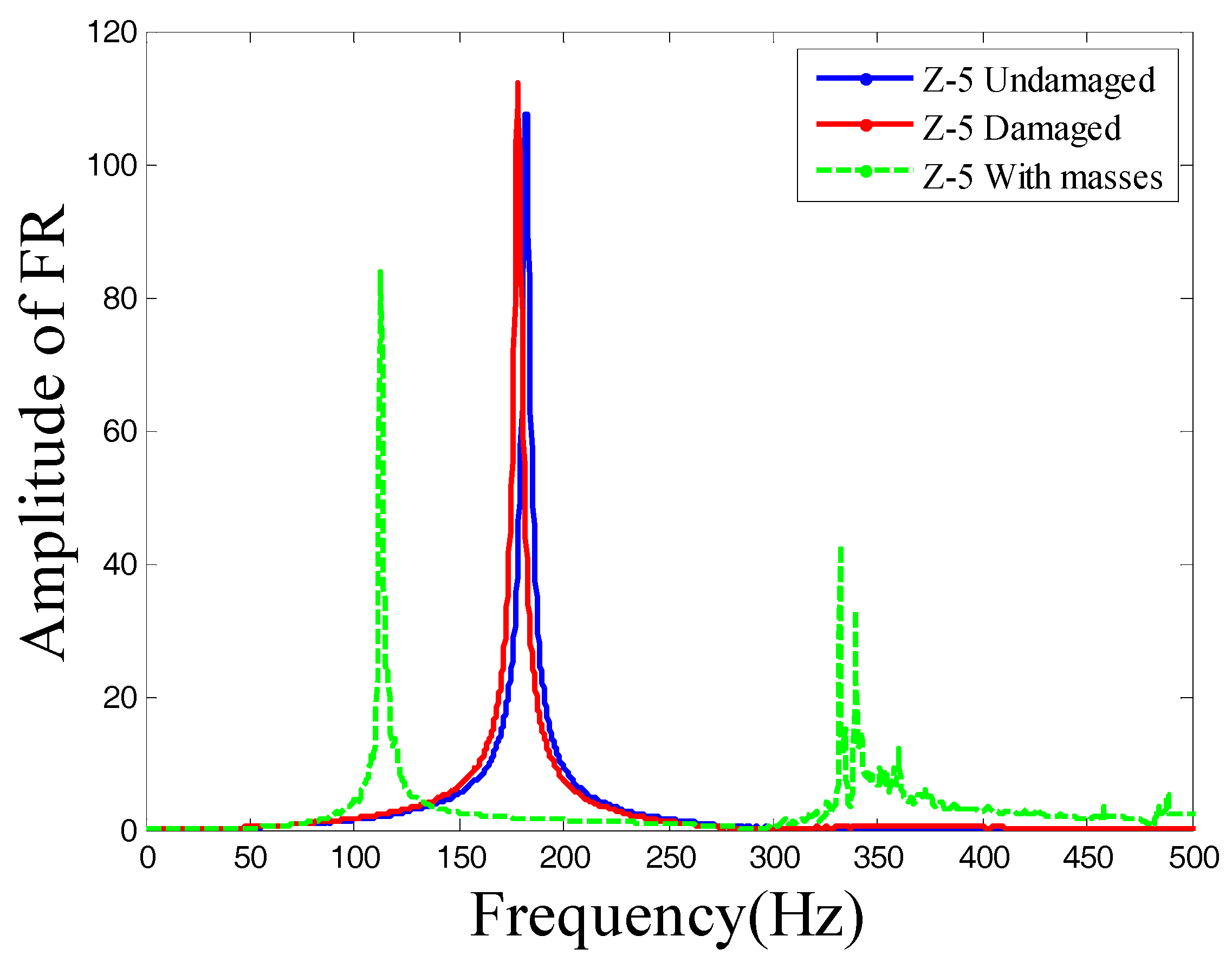
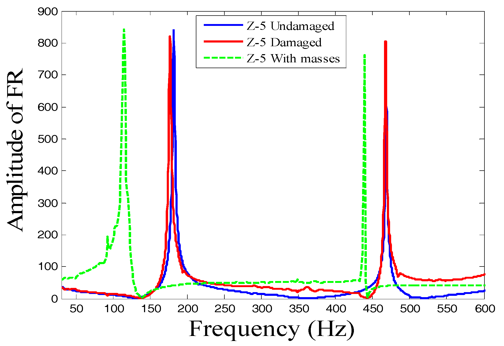
Damage to substructure 5 is found facing the ground and the acceleration sensor is disposed on the upper surface of the pipe facing the hole. The excitation point of the hammer is near the sensor, as shown in Figure 18. The positions of the acceleration sensor and hammer excitation are sequentially moved to measure the response of the 10 substructures. Figure 19 shows the frequency response of the damage to substructure 5 where a comparison of the undamaged pipe and damaged structure with additional 8 kg of virtual masses is shown as well. The first frequency is seen to decrease from 181.9 Hz to 177.3 Hz after the damage. With the addition of 8 kg virtual mass, the frequency changed to 115.1 Hz.
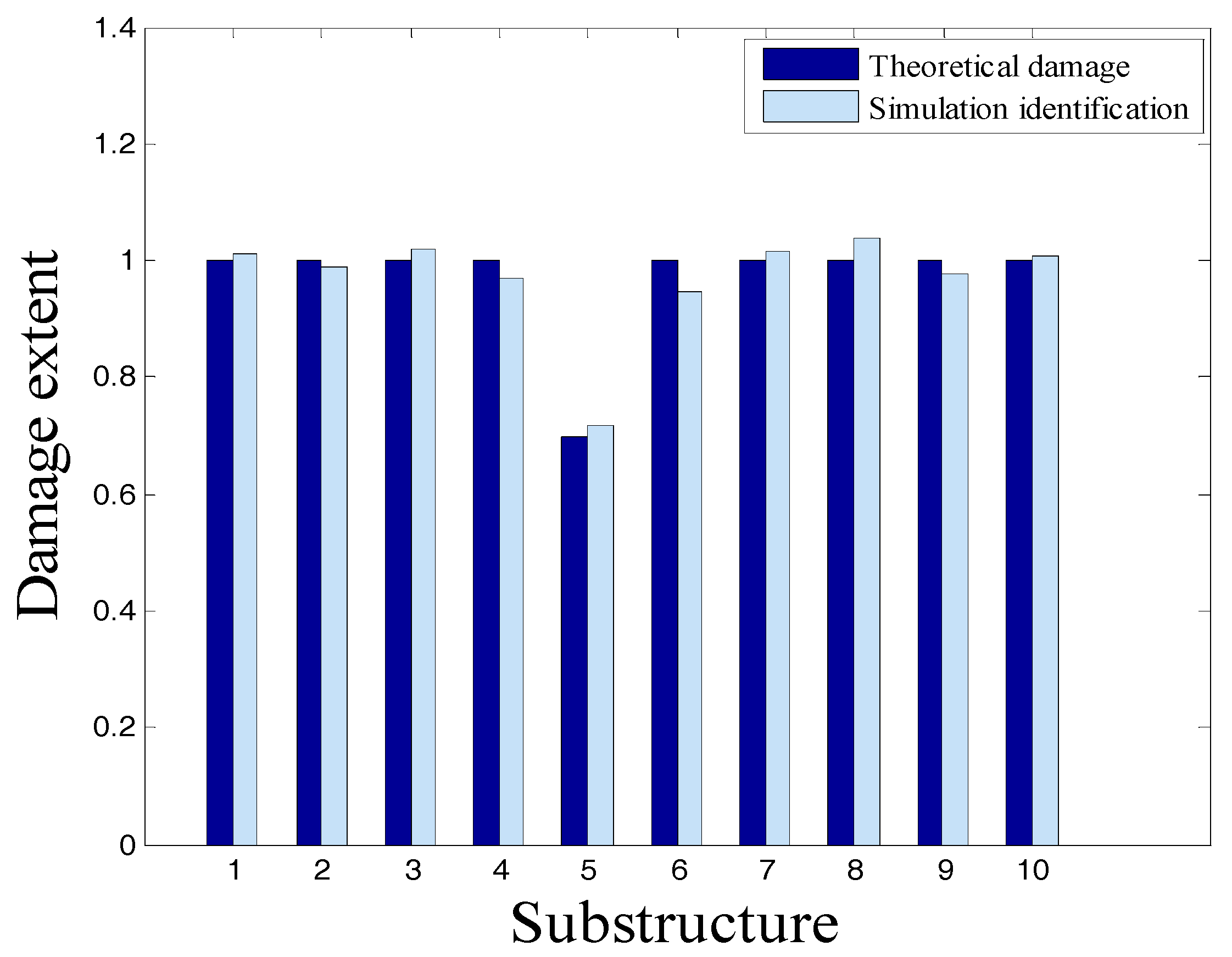
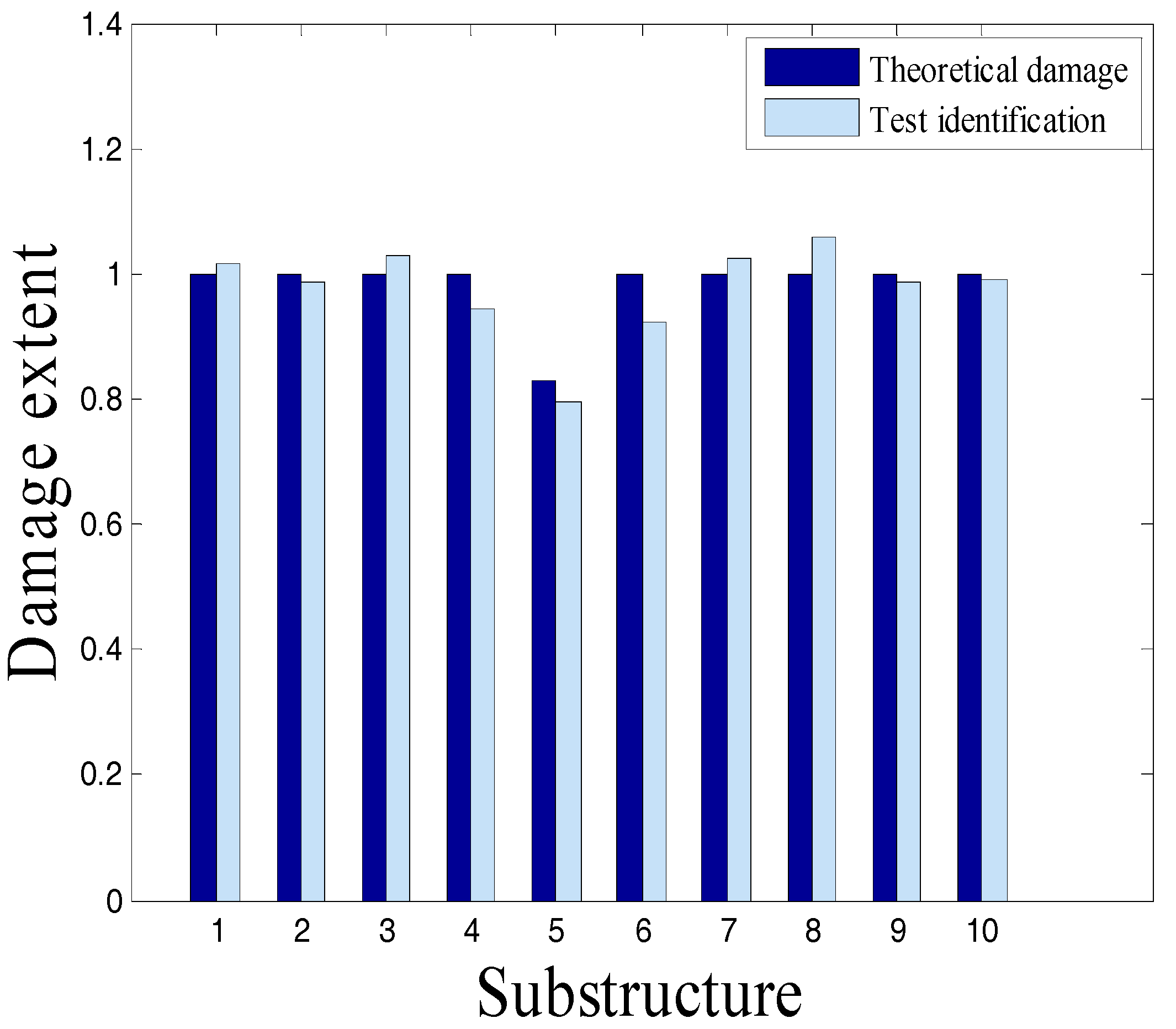
The measured responses of the 10 substructures are substituted into the additional virtual mass formula to obtain the first frequency with the additional optimal masses. Then, the damage factor of the substructure can be iterated according to Equation (10), which is combined with the sensitivity matrix of theoretical FEM, as shown in Figure 20. In the experimental results, the damage to substructure 5 is reduced to 0.80 by the iteration, which is close to the theoretical calculation value of 0.83. This scenario indicates that the damage identification method is successful. At the same time, the iterated results of other substructures are close to 1.0, indicating that the structure is intact and consistent with the experimental model.
5. Conclusions
This paper proposes an effective method for pipeline damage identification by constructing virtual structures with additional virtual masses. The virtual structures are constructed to increase their sensitivity with respect to the considered damage parameters. Through numerical simulation and test verification, the damage identification of the pipeline can be realized. We summarize the most important features below:
- (1)
- Based on the concept of VDM, we propose a method of adding virtual masses to the structure. The great advantage is that it evades practical difficulties of adding real mass to the structure, thus reducing the negative effect of real masses on the structure itself and making the actual operation flexible and convenient.
- (2)
- By constructing the virtual structure on the pipeline with the additional virtual masses, the frequency of high relative sensitivity can be selected and combined with a diagonally dominant sensitivity matrix as well as with frequency changes before and after damage. Hence, the degree of damage on the substructure can be accurately identified.
- (3)
- Damage identification of global structures requires only two sensors: excitation and acceleration, which are sequentially used for constructing the considered virtual structures one by one. Therefore, the experimental costs can be significantly reduced.
Acknowledgments
The authors are grateful for the financial support from the National Key Research and Development Program of China (Project No. 2017YFC0703410), and National Natural Science Foundation of China (NSFC) under Grant Nos. 51478079, the Fundamental Research Funds for the Central Universities (DUT16LK10).
Author Contributions
To complete this article, the whole team worked together and each of them made outstanding contributions. Jilin Hou provided the theoretical support. Dongsheng Li and Dang Lu conceived and designed the experiments.Dang Lu performed the experiments. Dongsheng Li and Dang Lu analyzed the data. Jilin Hou contributed acquisition program and analysis tools. Dongsheng Li and Dang Lu wrote the paper.
Conflicts of Interest
The authors declare no conflict of interest. The founding sponsors had no role in the design of the study; in the collection, analyses, or interpretation of data; in the writing of the manuscript, and in the decision to publish the results.
References
- Han, H.; Zhou, S.; Hao, Z.; Zhang, L. School of Mechanical and Power Engineering, East China University of Science and Technology. Study on identification of pipe damage based on strain modal difference. Vib. Meas. Diagn. 2013, 33, 210. [Google Scholar]
- Li, H.; Tao, H. Damage location method of pressure pipeline based on frequency variation square ratio. J. Dalian Univ. Technol. 2002, 42, 400–403. [Google Scholar]
- Pandey, A.K.; Biswas, M. Experimental verification of flexibility difference method for locating damage in structures. J. Sound Vib. 1995, 184, 311–328. [Google Scholar]
- Hao, Z.; Zhou, S. Damage Identification of Pipeline Based on Curvature Modal and Optimization Algorithm; East China University of Science and Technology: Shanghai, China, 2014; pp. 2–10. [Google Scholar]
- Ren, Q.; Li, H. Undamaged detection of pipe based on modal varied quotiety of strain. J. Dalian Univ. Technol. 2001, 41, 648–652. [Google Scholar]
- Zhang, Q.; Jankowski, L.; Duan, Z. Damage identification using substructural virtual distortion method. Proc SPIE 2012, 8345, 110. [Google Scholar]
- Khan, F.; Bartoli, I.; Vanniamparambil, P.A.; Carmi, R.; Rajaram, S.; Kontsos, A. Integrated Health Monitoring System for Damage Detection in Civil Structural Components; CRC Press: London, UK, 2014; pp. 307–313. [Google Scholar]
- Demz, K.; Mroz, Z. Damage identification using modal, static and thermographic analysis with additional control parameters. Comput. Struct. 2010, 88, 1254–1264. [Google Scholar]
- Dinh, H.; Nagayama, T.; Fujino, Y. Structural parameter identification by use of additional known masses and its experimental application. Struct. Control Health Monit. 2012, 19, 436–450. [Google Scholar]
- Nalitolela, N.; Penny, J.; Friswell, M. A mass or stiffness addition technique for structural parameter updating modal analysis. Int. J. Anal. Exp. Modal Anal. 1992, 7, 157–168. [Google Scholar]
- Kołakowski, P.; Wikło, M.; Holnicki-Szulc, J. The virtual distortion method—A versatile reanalysis tool for structures and systems. Struct. Multidiscip. Optim. 2008, 36, 217–234. [Google Scholar]
- Suwala, G.; Jankowskiy, L. A model-free method for identification of mass modifications. Struct. Control Health Monit. 2012, 19, 216–230. [Google Scholar]
- Hou, J.; Jankowski, Ł.; Ou, J. Structural damage identification by adding virtual masses. Struct. Multidisc. Optim. 2013, 48, 59–72. [Google Scholar]
- Zhang, Q.; Jankowski, Ł.; Duan, Z. Simultaneous identification of moving masses and structural damage. Struct. Multidiscip. Optim. 2010, 42, 907–922. [Google Scholar]
- Świercz, A.; Kołakowski, P.; Holnicki-Szulc, J. Damage identification in skeletal structures using the virtual distortion method in frequency domain. Mech. Syst. Signal Process. 2008, 22, 1826–1839. [Google Scholar]
- Hou, J.; Wang, Z. Structural damage identification method based on additional virtual masses. J. Comput. Mech. 2013, 30, 770–776. [Google Scholar]
- Liu, J.; Yang, Q.; Zou, T. On the model reduction techniques in structural damage identification. J. Sun Yat-sen Univ. (Nat. Sci. Ed.) 2006, 45, 1–8. [Google Scholar]
- Hou, J.; Jankowski, Ł.; Ou, J. Model Updating Based on Substructure Isolation Methods; Harbin Institute of Technology: Harbin, China, 2012; pp. 146–150. [Google Scholar]
Figure 1.
Pipe substructure number.
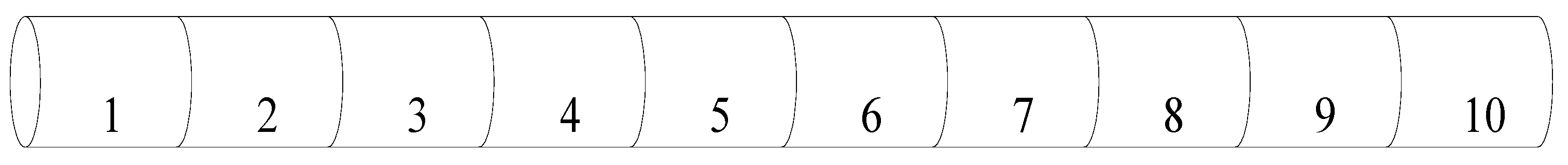
Figure 2.
The first four mode shapes. (a) The 1st mode shape; (b) The 2nd mode shape; (c) The 3rd mode shape; (d) The 4th mode shape.
Figure 2.
The first four mode shapes. (a) The 1st mode shape; (b) The 2nd mode shape; (c) The 3rd mode shape; (d) The 4th mode shape.

Figure 3.
Relationship between relative sensitivity and mass. (a) Substructure: 1/2/9/10; (b) Substructure: 3/8; (c) Substructure: 4/7; (d) Substructure: 5/6.
Figure 3.
Relationship between relative sensitivity and mass. (a) Substructure: 1/2/9/10; (b) Substructure: 3/8; (c) Substructure: 4/7; (d) Substructure: 5/6.
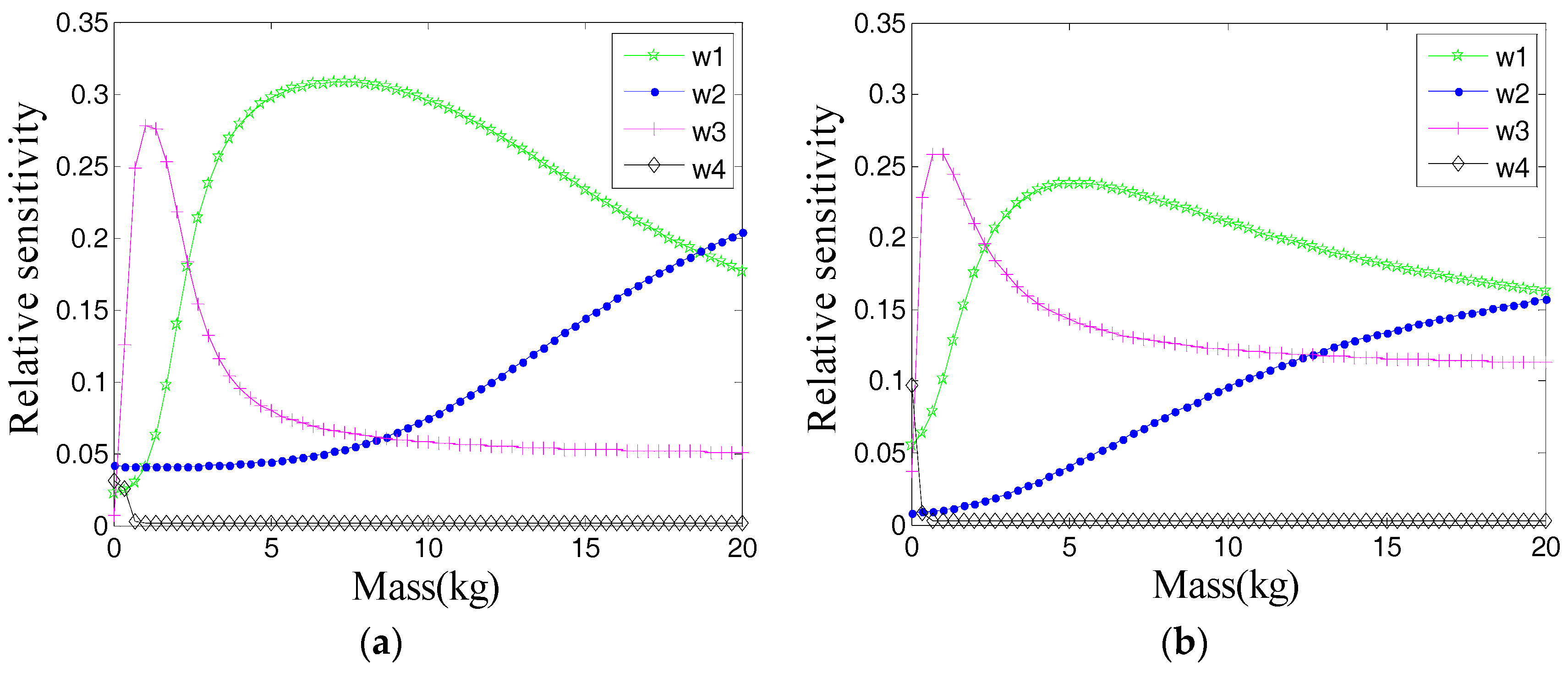
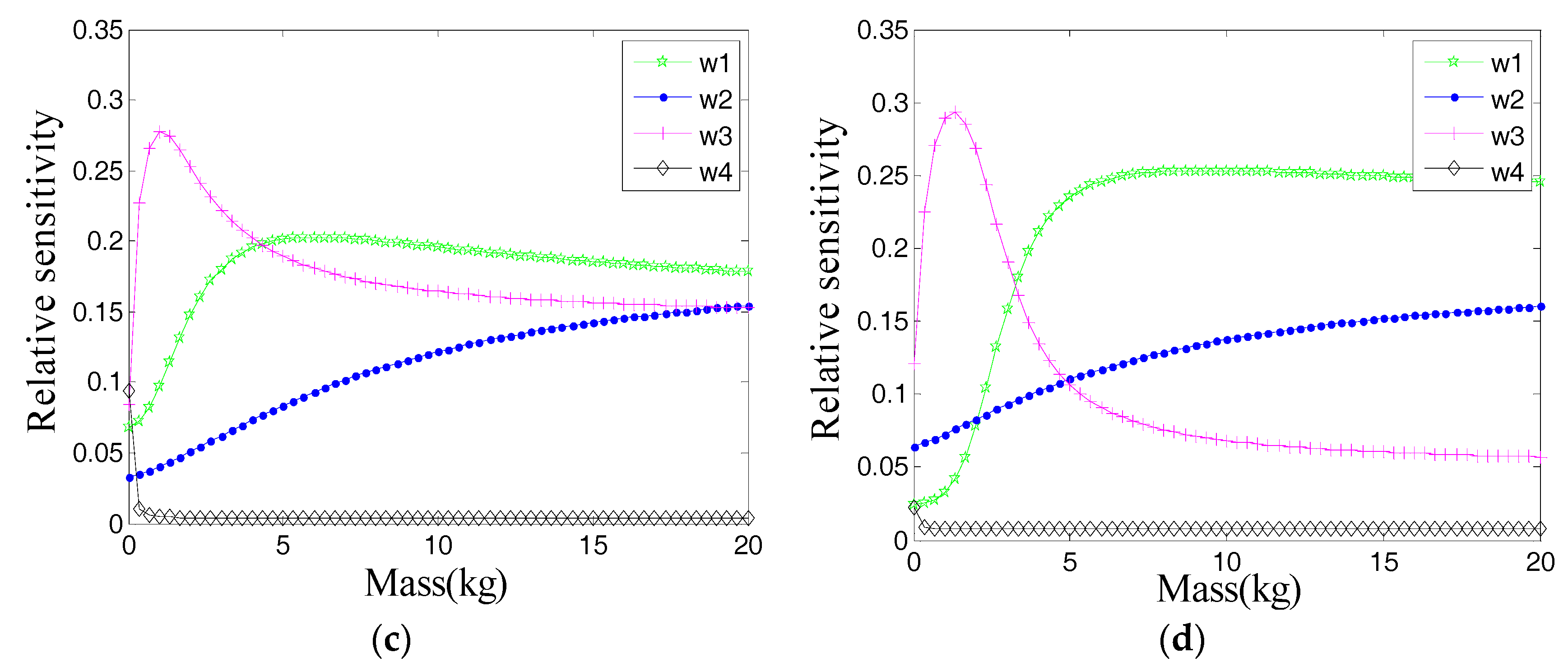
Figure 4.
Simulated excitation.

Figure 5.
Acceleration response.
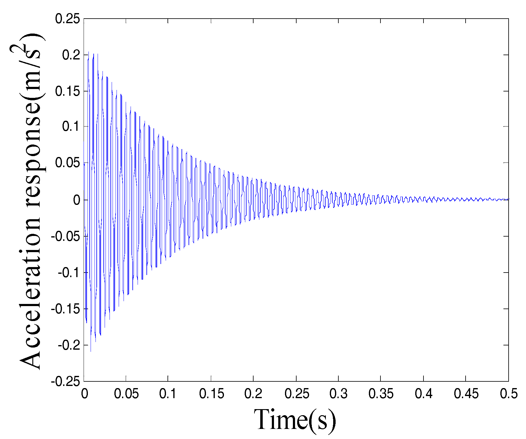
Figure 6.
Frequency response.
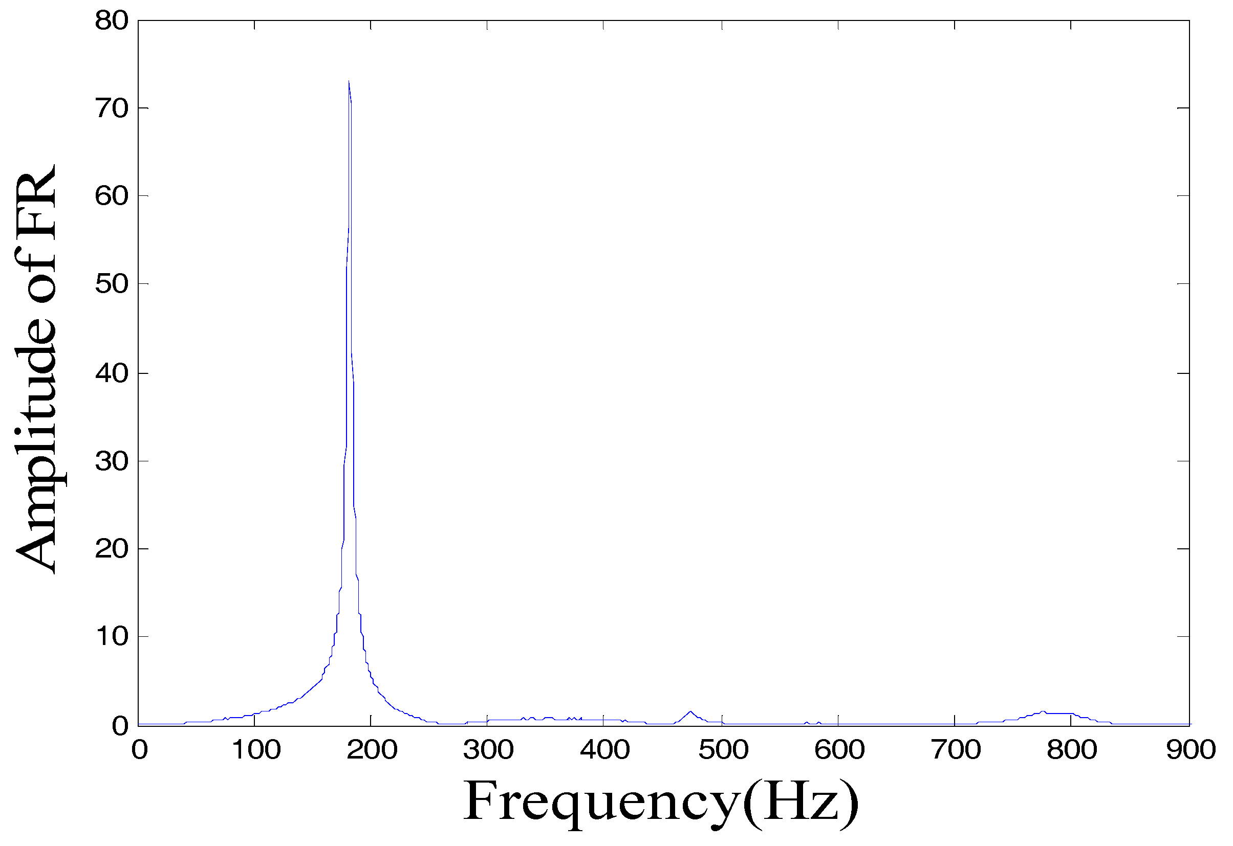
Figure 7.
Nephogram of frequency response with respect to virtual mass.

Figure 8.
Changes of the first frequency with different masses (FEM).
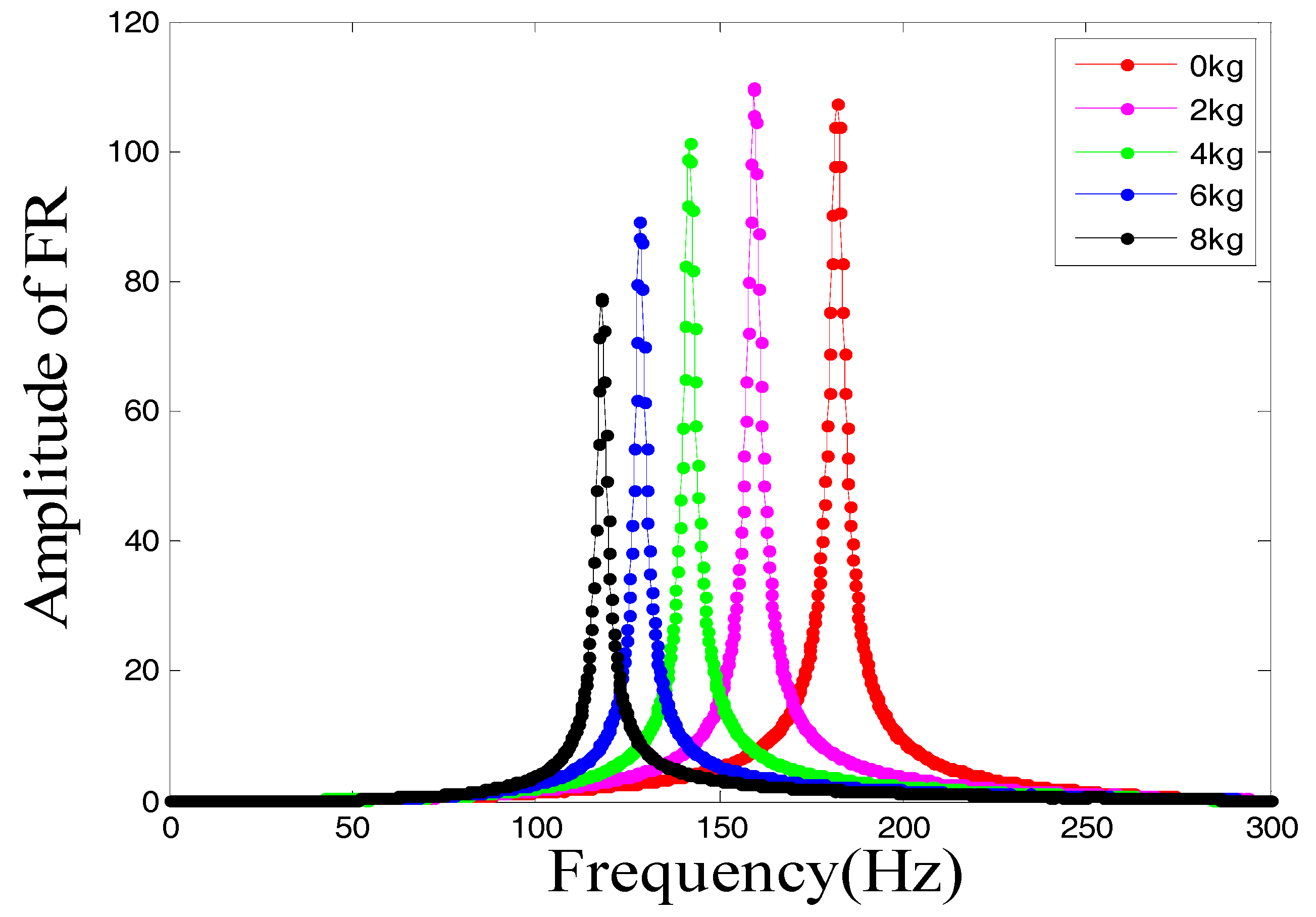
Figure 9.
Changes of the first frequency with different masses (VDM).
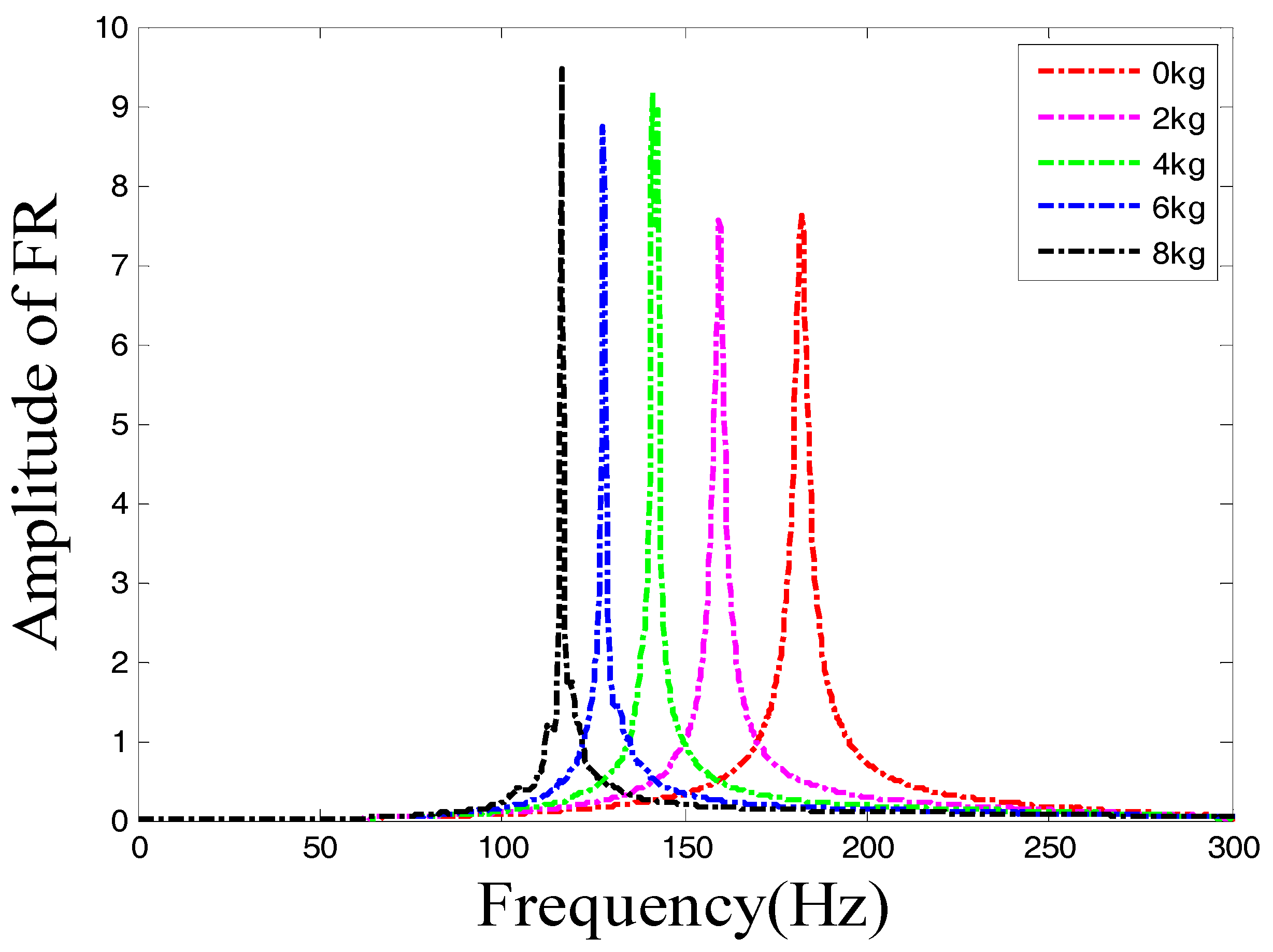
Figure 10.
Substructure 5: Frequency changes before and after damage.

Figure 11.
Case 1: identified damage extents.

Figure 12.
Case 2: identified extents of damage.
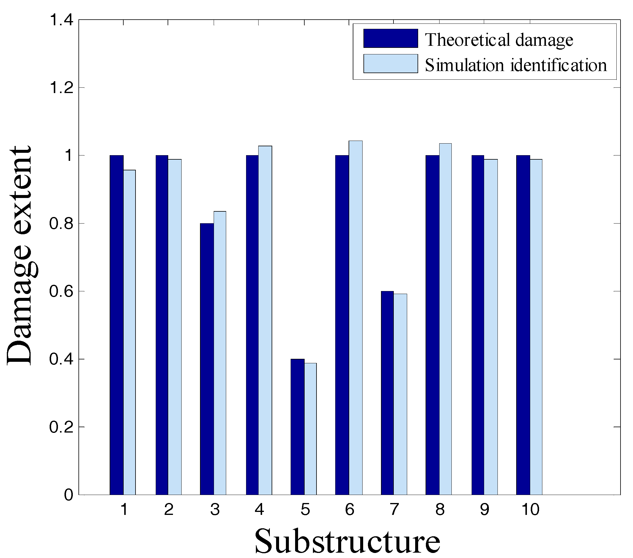
Figure 13.
Test model of the pipe structure.
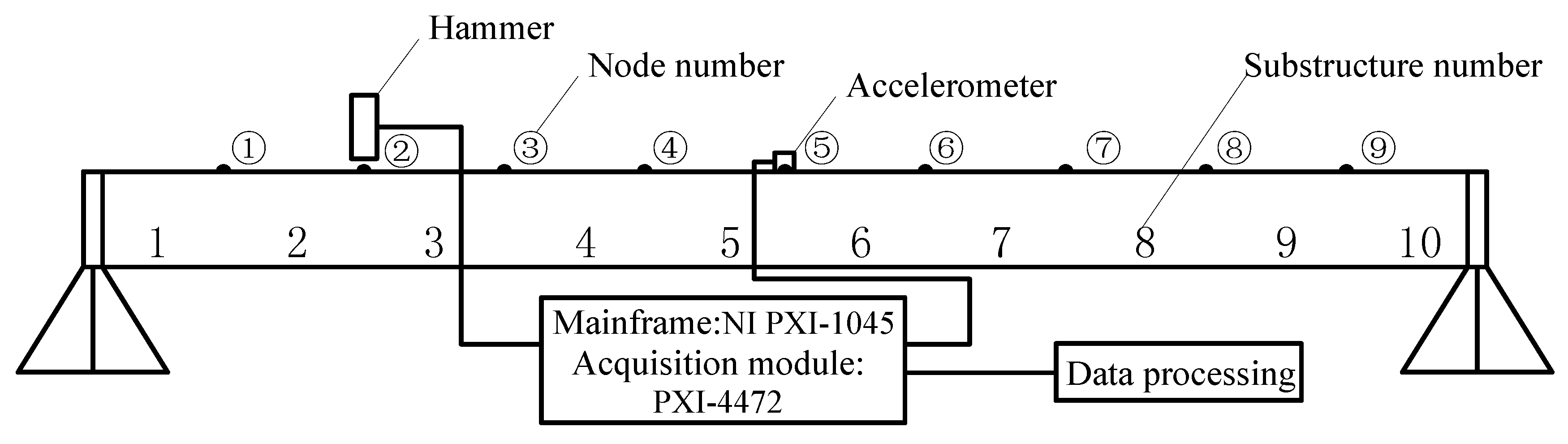
Figure 14.
Test model of actual pipeline. (a) Test pipeline; (b) Hammer excitation.

Figure 15.
Measured test results. (a) Measured excitation; (b) Acceleration response.
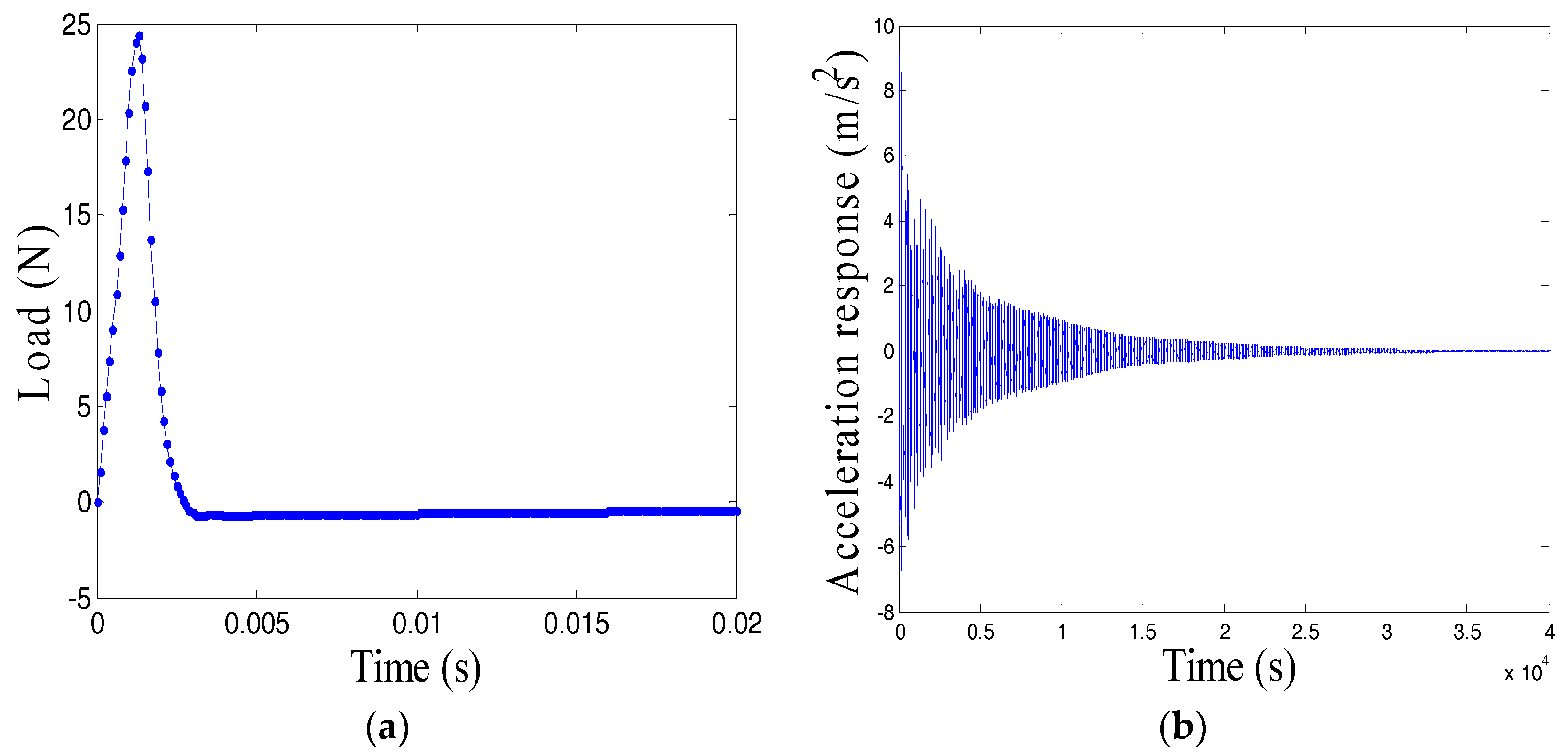
Figure 16.
Frequency response.

Figure 17.
Substructure 5: damage size (unit: cm). (a) Damage section; (b) Hole size.

Figure 18.
Actual damage and measured response. (a) Damage hole; (b) Hammer excitation.
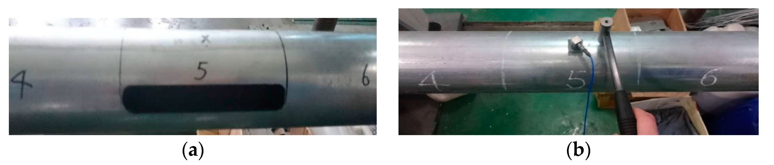
Figure 19.
Sub-structure 5: The measured frequency response.

Figure 20.
The test damage identification.


Table 1.
Pipe parameters.
| Type | Length/m | Outside Diameter/mm | Thickness/mm | Elastic Modulus/Gpa | Poisson’s Ratio | Density/kg/m3 |
|---|---|---|---|---|---|---|
| Straight pipe | 2 | 114 | 3 | 205 | 0.3 | 7850 |
Table 2.
The first four natural frequencies/Hz.
| Order | 1 | 2 | 3 | 4 |
|---|---|---|---|---|
| Frequency | 181.99 | 476.51 | 793.92 | 813.22 |
Table 3.
The first four natural frequencies after reduction/Hz.
| Order | 1 | 2 | 3 | 4 |
|---|---|---|---|---|
| Frequency | 182.24 | 476.79 | 795.07 | 814.57 |
Table 4.
Ten groups of virtual structures.
| Virtual Structure | G1 | G2 | G3 | G4 | G5 | G6 | G7 | G8 | G9 | G10 |
|---|---|---|---|---|---|---|---|---|---|---|
| Substructure | 1 | 2 | 3 | 4 | 5 | 6 | 7 | 8 | 9 | 10 |
| Order | 1 | 1 | 1 | 1 | 1 | 1 | 1 | 1 | 1 | 1 |
| Mass (kg) | 7 | 7 | 5 | 6 | 8 | 8 | 6 | 5 | 7 | 7 |
Table 5.
Frequency comparison of ten virtual structures.
| Virtual Structure | G1 | G2 | G3 | G4 | G5 | G6 | G7 | G8 | G9 | G10 |
|---|---|---|---|---|---|---|---|---|---|---|
| Mass (kg) | 7 | 7 | 5 | 6 | 8 | 8 | 6 | 5 | 7 | 7 |
| FEM (Hz) | 177.38 | 175.86 | 161.12 | 137.43 | 117.87 | 118.07 | 137.63 | 161.47 | 175.70 | 177.26 |
| VDM (Hz) | 177.43 | 175.51 | 160.79 | 137.62 | 117.54 | 118.15 | 137.91 | 161.09 | 175.48 | 177.54 |
Table 6.
Theoretical damage vectors of case 2.
| Substructure | 1 | 2 | 3 | 4 | 5 | 6 | 7 | 8 | 9 | 10 |
|---|---|---|---|---|---|---|---|---|---|---|
| Damage vector: | 1.0 | 1.0 | 0.8 | 1.0 | 0.4 | 1.0 | 0.6 | 1.0 | 1.0 | 1.0 |
Table 7.
The pipe: comparison of the measured and modeling frequencies.
| Order of Natural Frequency | Measured Frequency/Hz | Modeling Frequency/Hz | Error/% |
|---|---|---|---|
| 1st | 181.93 | 182.24 | 0.17 |
| 2nd | 473.68 | 476.79 | 0.66 |
© 2017 by the authors. Licensee MDPI, Basel, Switzerland. This article is an open access article distributed under the terms and conditions of the Creative Commons Attribution (CC BY) license (http://creativecommons.org/licenses/by/4.0/).
Share and Cite
MDPI and ACS Style
Li, D.; Lu, D.; Hou, J. Pipeline Damage Identification Based on Additional Virtual Masses. Appl. Sci. 2017, 7, 1040. https://doi.org/10.3390/app7101040
AMA Style
Li D, Lu D, Hou J. Pipeline Damage Identification Based on Additional Virtual Masses. Applied Sciences. 2017; 7(10):1040. https://doi.org/10.3390/app7101040
Chicago/Turabian StyleLi, Dongsheng, Dang Lu, and Jilin Hou. 2017. "Pipeline Damage Identification Based on Additional Virtual Masses" Applied Sciences 7, no. 10: 1040. https://doi.org/10.3390/app7101040
Note that from the first issue of 2016, this journal uses article numbers instead of page numbers. See further details here.