Application of Deep Networks to Oil Spill Detection Using Polarimetric Synthetic Aperture Radar Images

1
Faculty of Information Technology, Beijing University of Technology, Beijing 100124, China
2
National Astronomical Observatories, Chinese Academy of Sciences, Beijing 100012, China
3
Key Laboratory of Lunar Science and Deep-space Exploration, Chinese Academy of Sciences, Beijing 100012, China
*
Authors to whom correspondence should be addressed.
Appl. Sci. 2017, 7(10), 968; https://doi.org/10.3390/app7100968
Submission received: 29 July 2017
/
Revised: 10 September 2017
/
Accepted: 15 September 2017
/
Published: 21 September 2017
(This article belongs to the Special Issue Application of Artificial Neural Networks in Geoinformatics)
Abstract
:Featured Application
Using polarimetric synthetic aperture radar (SAR) remote sensing to detect and classify sea surface oil spills, for the early warning and monitoring of marine oil spill pollution.
Abstract
Polarimetric synthetic aperture radar (SAR) remote sensing provides an outstanding tool in oil spill detection and classification, for its advantages in distinguishing mineral oil and biogenic lookalikes. Various features can be extracted from polarimetric SAR data. The large number and correlated nature of polarimetric SAR features make the selection and optimization of these features impact on the performance of oil spill classification algorithms. In this paper, deep learning algorithms such as the stacked autoencoder (SAE) and deep belief network (DBN) are applied to optimize the polarimetric feature sets and reduce the feature dimension through layer-wise unsupervised pre-training. An experiment was conducted on RADARSAT-2 quad-polarimetric SAR image acquired during the Norwegian oil-on-water exercise of 2011, in which verified mineral, emulsions, and biogenic slicks were analyzed. The results show that oil spill classification achieved by deep networks outperformed both support vector machine (SVM) and traditional artificial neural networks (ANN) with similar parameter settings, especially when the number of training data samples is limited.
1. Introduction
As one of the most significant sources of marine pollution, oil spills have caused serious environmental and economic impacts to the ocean and coastal zone [1]. Oil spills near the coast can be caused by ship accidents, explosion of oil rig platforms, broken pipelines, and deliberate discharge of tank-cleaning wastewater from ships. The NEREIDs program, sponsored by the European Commission, was the first robust attempt to use shipping, geological and metocean data to characterize oil spills in one of the major oil exploration areas of the world, prior to any major oil spill accident. Based on this data, oil spill models were established to simulate the development and trajectories of oil spills and investigate the susceptibility of coastal zone and find suitable measures to alleviate its impacts to the environment [2,3,4,5].
Early warning and near-real-time monitoring of oil slicks plays a very important role in cleaning up operation of oil spill to alleviate its impact to coastal environment [2,3]. Synthetic aperture radar (SAR) is one of most promising remote sensing systems for oil spill monitoring, for it can provide valuable information about the position and size of the oil spill [1]. Moreover, the wide coverage and all-day, all-weather capabilities make SAR very suitable for large scale oil spill monitoring and early warning [6,7,8].
In their early stages, studies of oil spill detection are mainly based on single polarimetric SAR images [9,10,11,12]. The theoretical rationale of SAR oil spill detection is that the presence of oil slicks on the sea surface dampens short-gravity and capillary waves, so the Bragg scattering from the sea surface is largely weakened. The ideal sea surface wind speed for oil spills detection is 3–14 m/s [13]. As a result, oil spills can be detected as “dark” areas in SAR images. However, some other manmade or natural phenomena can result in very similar low scattering areas on the sea surface, e.g., biogenic slicks, waves, currents and low-wind areas, etc. Conventional oil spill detection procedures use intensity, morphological texture, and auxiliary information to distinguish mineral oil and its lookalikes, with its processing chain divided into three main steps [13]: (1) dark spot detection; (2) features extraction; and (3) classification between mineral and its lookalikes.
Single polarimetric SAR-based oil spill detection algorithms need auxiliary information and large number of data samples to classify mineral oil and its lookalikes. Sometimes the shape and texture of oil slicks may vary, affecting the robustness of intensity-based oil spill classification algorithms. Polarimetric observation capabilities provided by advanced SAR sensors have much stronger capabilities for oil spills detection [14]. For instance, biogenic slicks and mineral oil are difficult to distinguish by single polarimetric SAR images. Yet, their polarimetric scattering mechanisms are largely different: for oil-covered areas, Bragg scattering is largely suppressed, and high polarimetric entropy can be documented. In the case of a biogenic slick, Bragg scattering is still dominant, but with a low intensity. Thus, similar polarimetric behaviors as those of oil-free areas should be expected in the presence of biogenic films. Hence, polarimetric features can largely help the image classification between mineral and biogenic lookalikes [14].
Various polarimetric features have been proposed to classify oil spills. The standard deviation of copolarized phase difference (phase difference between Vertical transmit and Vertical receive-VV and Horizonal transmit and Horizonal receive-HH channel) has shown a strong oil classification capability on C-, X-, and L-band data [15]. Nunziata et al. (2011) proposed pedestal height to describe the different polarization signature between mineral oil and biogenic lookalikes [16]. Minchew et al. (2012) took the advantage of copolarization ratio to study the mixing status of crude oil and sea water [17]. Zhang et al. (2011) used the conformity coefficient as a binary classifier [18]. Other polarimetric features such as degree of polarization, entropy, alpha angle, and Bragg likelihood angle were also used to classify oil spills [19,20,21].
Some previous studies conducted automatic oil-spill classification algorithms. Marghany (2001) developed models to discriminate textures between oil and water by using co-occurrence textures [22]. Gambardella et al. (2008) proposed one-class classification with an optimized feature selection algorithm and obtained a promising oil spill classification [23]. Frate et al. (2000) proposed a semiautomatic detection of oil spills by neural network [24]. Garcia-Pineda et al. (2008) developed the Textural Classifier Neural Network Algorithm (TCNNA) to map an oil spill in the Gulf of Mexico Deepwater Horizon accident [11]. Marghany (2013) used a genetic algorithm (GA) for automatic detection of an oil spill from ENVISAT ASAR (Advanced Synthetic Aperture Radar) data [25]. Li et al. (2013) used a Support Vector Machine (SVM) to detect oil spills based on morphological features on very limited data samples [26].
Polarimetric SAR features contain massive complementary and redundancy information. The extraction and optimization of them are closely related to the performance of oil spill classification [27]. Deep learning algorithms have very strong capabilities of exploring complex correlation between features and achieve very promising fitting result on complicated problems. It has been a very popular technique for image processing, computer vision, and natural language processing. According to the authors, deep learning has not been used in features optimization for oil spills detection based on polarimetric SAR data, and it should be a very promising research topic.
Deep neural network with multilayer neuron has powerful capabilities in describing complex functions compared with shallow networks [28]. However, the traditional gradient descent technique works poorly on a deep neural network when the weights are initialized randomly. The reason is that when the derivative is calculated using the back propagation method, the magnitude of the gradient (from the output layer to the initial layer of the network) decreases dramatically as the network depth increases. As the result, the gradient of the overall loss function, with respect to the weights of the first few layers, is very small. Thus, when the gradient descent method is used, the weights of the first layers change very slowly, so that they cannot learn effectively from the samples. This problem is often referred to as “gradient dispersion”. In 2006, Hinton et al. proposed the deep belief network (DBN), which is a belief network composed of Restricted Boltzmann Machine (RBM) one layer at a time, to take the advantage of complementary priors of the data. Inspired by DBN, Beigio et al. (2006) used a stacked autoencoder, which is a deep multilayer neural network that initialized its weights by a greedy layer-wise unsupervised training strategy [29].
Moreover, feature dimension reduction can be seen as an early fusion step. Fusion at different stages of classification procedures is a booming research field that has shown capabilities for improvement of classification results. For instance, Vergara et al. fused the output of nonindependent detectors to derive the optimum classification result [30]. Late fusion of scores of several classifiers could be adapted to the proposed problem as a future research work.
The aims of this paper are exploring the capabilities of deep learning algorithms on polarimetric SAR-based marine oil spill detection. In Section 2, research methods including the representation of polarimetric SAR data, feature extraction methods and deep learning algorithms including DBN and SAE will be introduced. In Section 3, experiments were conducted on RADARSAT-2 data containing verified oil spills and biogenic lookalikes. The performance of different algorithms on various sample sizes for oil spill classification will be compared. Finally, conclusions are drawn in Section 4, and the significance and future work of the study will be briefly presented.
2. Methods
2.1. Foudamentals of Polarimetric SAR
The scattering characteristics of the observed target can be described by matrix, S; which links the scattered and incident electromagnet field, in the backscattered coordinate system:
where k is the wavenumber of the EM wave, r is the distance.
Fully polarimetric SAR observations can be achieved by quad-polarimetric mode, in which both horizontal and vertical polarized signals are transmitted alternatively and received coherently. The 2 × 2 scattering matrix is used to represent the single look complex quad-pol SAR data:
where Sij describes the transmitted and received polarization, respectively, with h denoting the horizontal direction and v denoting the vertical direction.
To take advantage of statistical properties and reduce the effect of speckle noise of SAR data, covariance matrix is often derived from the scattering matrix by multilook its second order products:
where “*” is the symbol of conjugate, and “< >“ stands for multilook by using an averaging window. Multilook is applied as a standard procedure to obtain the second order statistics (covariance matrix, coherence matrix) of the SAR data, an average window of 5 × 5 is normally used for balancing the multilook result and maintaining the spatial resolution.
2.2. Features Extraction for Oil Spills Detection
Previous studies proved experimentally that various SAR features could assist oil spill detection and classifications [31]. In this study, ten features including single VV channel intensity, entropy, alpha angle, degree of polarization, ellipticity, pedestal height, copolarized phase difference (CPD), conformity coefficient, correlation coefficient and coherence coefficient are extracted from the covariance matrix (or coherence matrix and Stokes vector deriving from the covariance matrix) [32] of polarimetric SAR data. The ten features investigated in this study, and their behavior on clean sea surface and sea surface covered by different materials, are given in Table 1. Detailed definitions and their behavior on different targets are provided explicitly in [27].
2.3. Deep Belief Network (DBN)
2.3.1. Restricted Boltzmann Machine
RBM is a neural perceptron consisting of visible and hidden layers, and the neurons between the visible layer (vi, i = 1, …, Nv) and the hidden layer (hj, j = 1, ..., Nh) are bidirectional and fully connected. The basic structure of RBM is shown in Figure 1:
In RBM, W represents the weight between any two connected neurons, in which each neuron has a bias coefficient b (of neurons) and c (of hidden neurons).
The energy of the RBM can be represented by:
And the probability of the activation of the hidden layer neuron hj is:
Similarly, the neurons in the visible layer can also be activated by the bidirectional connected hidden neurons:
where is the activation function, e.g., sigmoid function:
Since for RBM the neurons of the same layer is not connected, they are independent:
Based on the input data vector x, the possibility of the activation of each hidden layer neuron can be calculated. Similarly, based on the activation state of hidden layer neurons, the activation state of visible layers can be calculated. Through a contrastive divergence algorithm [28], the parameters of the RBM: (b, c, W) can be set based on the input data vector x iteratively by a Gibbs sampling technique. An RBM can be seen as a feature detector, which is often used for dimensional reduction of the data. The training process of RBM is to find a probability distribution that can best produce training samples.
2.3.2. The Structure of DBN
DBN is a generative model which establishes a joint distribution between a label and the data sample. It not only considers P (label/observation), but also P (observation/label). In a DBN, several RBMs are connected. The hidden layer of the previous RBM is the next RBM’s visible layer, and the output of the previous RBM is the input of the next RBM. During the pre-training process, the upper layer of RBM is trained before the training of the current layer. Usually when the top RBM is trained, the label information is also considered as the visible units.
2.3.3. The Fine-Tuning of DBN
Contrastive Wake-Sleep algorithms are usually used to fine-tune the pre-trained DBN. In the wake stage, the status of nodes of each layer is generated by external features and cognitive weights (upward), and the generated weights (downward) are modified using gradient descent algorithm. In the sleep stage, the state of the bottom neurons is generated through the top-level representation (the states learned by waking) and the weights generated in previous stage, then the cognitive weights of each layer are modified.
2.4. Stacked Autoencoder
2.4.1. Autoencoder
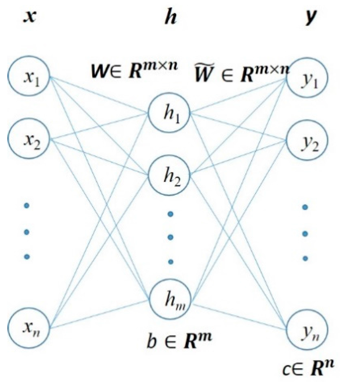
As shown in Figure 2, to build an autoencoder, three layers, namely, an input layer, a hidden layer and an output layer have to be established. The explanations of symbols used in Figure 2 are listed below:
- n: the size of the input and output layer.
- m: the size of the hidden layer.
- stand for the data vector of the input, hidden and output layers, respectively.
- stand for the bias vector of the hidden and output layers, respectively.
- stands for weights matrix between the input and hidden layer.
- stands for weights matrix between the hidden and input layer.
From the input layer to the output of hidden layer, the input signal is encoded. And from hidden layer to the output, the output of hidden layer is decoded by:
In Equations (10) and (11), f() and g() stand for the encoding and decoding functions, respectively. Sf and Sg are the corresponding activation functions of the encoder and decoder. sigmoid function can be chosen as the activation function and WT can be taken as the weights of the decoder.
Given input vectors, the autoencoder aims to minimize the difference between an input x and the output y. The reconstruction error can be described by the cross-entropy function:
For the training set, S; the average reconstruction error can hence be established as:
By minimizing , the parameter of the autoencoder can be fitted. The learning of an autoencoder does not need the label information, so it is an unsupervised procedure. The output of the hidden layer h can be seen as a representation of input x.
2.4.2. The Stacking of Autoencoders
In a SAE, autoencoders are stacked so that they take the output h(k) of one hidden layer of the former autoencoder as the input for its successive autoencoder. Each layer is trained by a greedy unsupervised layer-wise training strategy, and the upper layers are the representations of relevant high-level abstractions (Figure 3). Stacked autoencoders can establish the deep neural network more efficiently by initializing its weights in a region near its local minimum.
2.4.3. Fine-Tuning of the SAE
Normally the last layer of the SAE is connected to a classifier, it can be a neural network, Softmax classifier, SVM, etc. Finally, a fine-tuning process is also taken on either the whole network or only the classifier by taking the advantage of the label information through a supervised classification, using the back-propagation algorithm.
3. Experimental Results
3.1. The Experiment Data
In this study, RADARSAT-2 quad-pol SAR data acquired during the 2011 Norwegian oil-on-water experiment (59°59′ N, 2°27′ E) were used for analysis. The data was received at 17:27 of 8 June 2011 UTC in fine-quad polarimetric mode, with the spatial resolution of in range and azimuth directions. The incident angle of the image is 34.5–36.1° and the local wind speed is 1.6–3.3 m/s. For the convenience of processing and display, a data sample with pixels was picked from the single look complex (SLC) data. The pseudo RGB image of the RADARSAT-2 data on the Pauli basis are provided in Figure 4. In the scene, three verified slicks were present; from left to right, they were: biogenic film, emulsions and mineral oil [33]. The biogenic film was simulated by Radiagreen plant oil. Emulsions were made of Oseberg blend crude oil mixed with 5% IFO380 (Intermediate Fuel Oil), released 5 h before the radar acquisition. Additionally, the Balder crude oil was released 9 h before the radar acquisition [34].
3.2. The Experiment Procedure
The SLC quad-polarimetric SAR data was firstly multi-looked, and then the covariance matrix and coherency matrix of the data samples were generated. As mentioned before, 10 features are extracted and saved as a 10-dimension vector for each pixel.
As shown in Figure 5, the 24,000 data samples were picked up from the image, including 12,000 verified positive (mineral oil) and 12,000 negative (clean sea surface and biogenic slick) samples. The data samples were picked by squared boxes with the size of for convenience and keeping the purity of the sample, and then their order was shuffled.
In order to test the performance of different algorithms and avoid over-fitting, a six-fold cross-validation was applied. We first divided the training set into six subsets equally. Then the five-sixths of the data samples were used as training set and the rest were taken as testing set. Sequentially, we repeat the classification and another one-sixth data sample were used as testing set. The experiment was conducted six times until each instance of the whole training set is predicted once. Finally, the cross-validation accuracy is the overall percentage of data which are correctly classified.
In order to test the performance of these algorithms on smaller sample sizes, the whole dataset was divided into smaller groups. All the 24,000 data samples were divided into 5 and 25 groups randomly. Then classifications were conducted on these groups, namely 4000 training, 800 testing and 800 training, and 160 testing samples respectively. In the experiment, the classification accuracy of smaller sample size was obtained by averaging the classification result on each group respectively.
In the experiment, two previously introduced deep learning algorithms (i.e., DBN and SAE) were tested on their performance of oil spill detection and classification. In addition, two traditional supervised classifiers including neural network (NN) and SVM were compared.
LIBSVM-a library for Support Vector Machines [33] was used to implement the SVM algorithm. The parameters C and were derived by shrinking heuristics search technique. The neural network has ten input neurons, two hidden layers and two output neurons. The initialization of the former layers of deep learning algorithms SAE and DBN were carried out by unsupervised pretraining, and then the outputs were connected to a neural network with two output neurons.
3.3. Results and Discusion
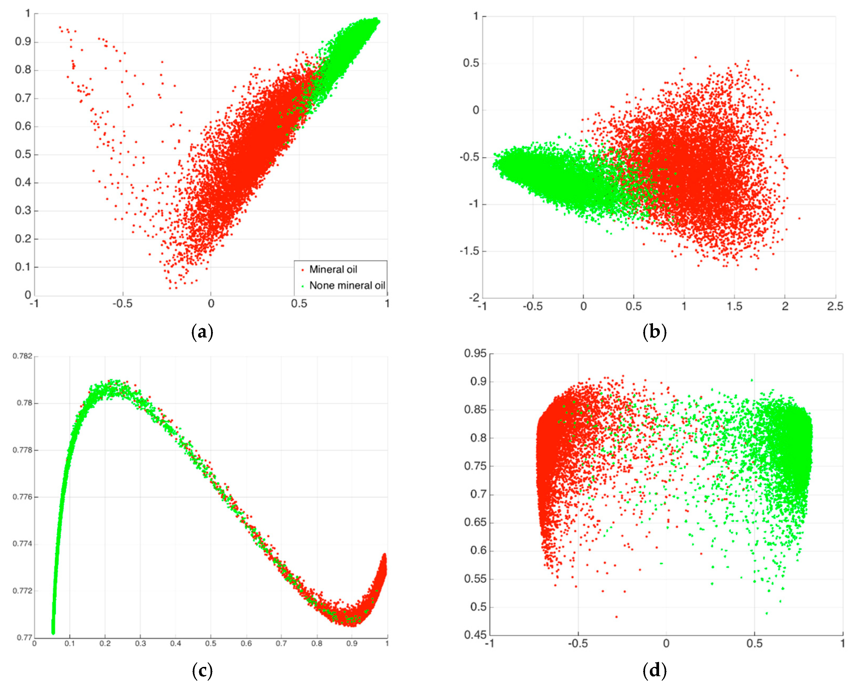
To examine the feature dimension reduction capability of the deep neural networks, scatter plots of the main original features and the features derived by principal component analysis (PCA), DBN and SAE are shown in Figure 6. Two of the most discriminative features, conformity coefficient and degree of polarization (DoP) of HH and VV transition/receiving combinations, as two of the most effective feature in oil spill classification [31], are plotted in Figure 6a. Scatter plots of the first two components derived by PCA are shown in Figure 6b. In this paper, taking the advantage of DBN and SAE, the dimension of polarimetric features are reduced to six, then they are put into fully connected neural network. To show these features in a scatter plot, PCA was implemented on the six features, and then the first two components are shown in Figure 6c,d. It can be observed that deep neural network algorithms effectively extracted the information from high dimensional features and improved their separability to distinguish mineral oil and none mineral samples.
The classification results are shown in Table 6 statistically, some key findings and discussions are listed as follow:
- SAE achieved the highest classification accuracy (lowest testing error) among all the algorithms on different sample sizes. DBN achieved a close performance to SAE. SAE and DBN applied in the experiment had similar structures and both of them took the advantage of greedy unsupervised layer-wise pretraining, so very similar performances were achieved. The unsupervised pretraining worked as a feature optimizer, which can reveal the latent relationship and reduction of noise in features. It helps to improve the performance of the followed supervised classification procedure.
- On the small training data set, deep learning algorithms have much higher performance than neural networks. When the number of data set is reduced, the parameters of traditional NN cannot be sufficiently tuned. Based on unsupervised pretraining, deep learning algorithms such as SAE and DBN have much stronger capability to achieve the optimized solution of the learning problem.
- When the number of data sample size is reduced, the classification error will increase (i.e., the accuracy is reduced). When the number of data sets reduced, the characteristics of the studied object cannot be sufficiently expressed by the limited number of data samples, so the classification performance is reduced.
- On the large training data set, NN have a close performance to deep learning algorithms. With large number of training data, the parameters of NN can be sufficiently adjusted. In this experiment, the NN have a few hidden layers, the gradient of objective function could pass to the layers in the front effectively. As the result, comparable classification performance was achieved by NN on large data set.
- SVM has better performance on small sample sizes than NN. SVM is based on structural risk minimization, which has superior performance on relative small data sets. It maximizes the classification margin, which is decided by a few support vectors and could successfully avoid the risk of the “curse of dimensionality”. However, although the SVM has several advantages, it is equivalent to a NN with one hidden layer, so on learning complicated relationships its performance is no better than the other three more complex classifiers applied in the experiment.
The confusion matrix of the cross-validation testing result is shown in Table 7, Table 8, Table 9 and Table 10. The best classification results were achieved by SAE on the largest data set: 20,000 training and 4000 testing samples. On the 24,000 testing set, 251 pixels were wrongly classified. 101 pixels of these 251 pixels were false positive (commission errors) and 150 pixels were false negative (omission errors). Similar false positive was achieved by DBN, with slightly higher false negative rate. In the confusion matrix achieved by NN and SAE, it can be discovered that compared with deep learning algorithms, they achieved lower false negative and higher false positive rates.
From the binary output that achieved by SAE (Figure 7), it can be observed that a few pixels in the area covered by the biogenic slick are classified as mineral oil. The possible reason of these “misclassifications” is the affection of signal noise on space-borne SAR data or the uniform distribution of the mineral oil and biogenic slicks. This misinterpretation can be further eliminated by a simple postprocessing step. Corrosion and swelling algorithms can be applied on the binary classification result to fix the small holes (missing alarm) in large oil-covered areas and isolated positive targets (false alarm) in the sea surface area.
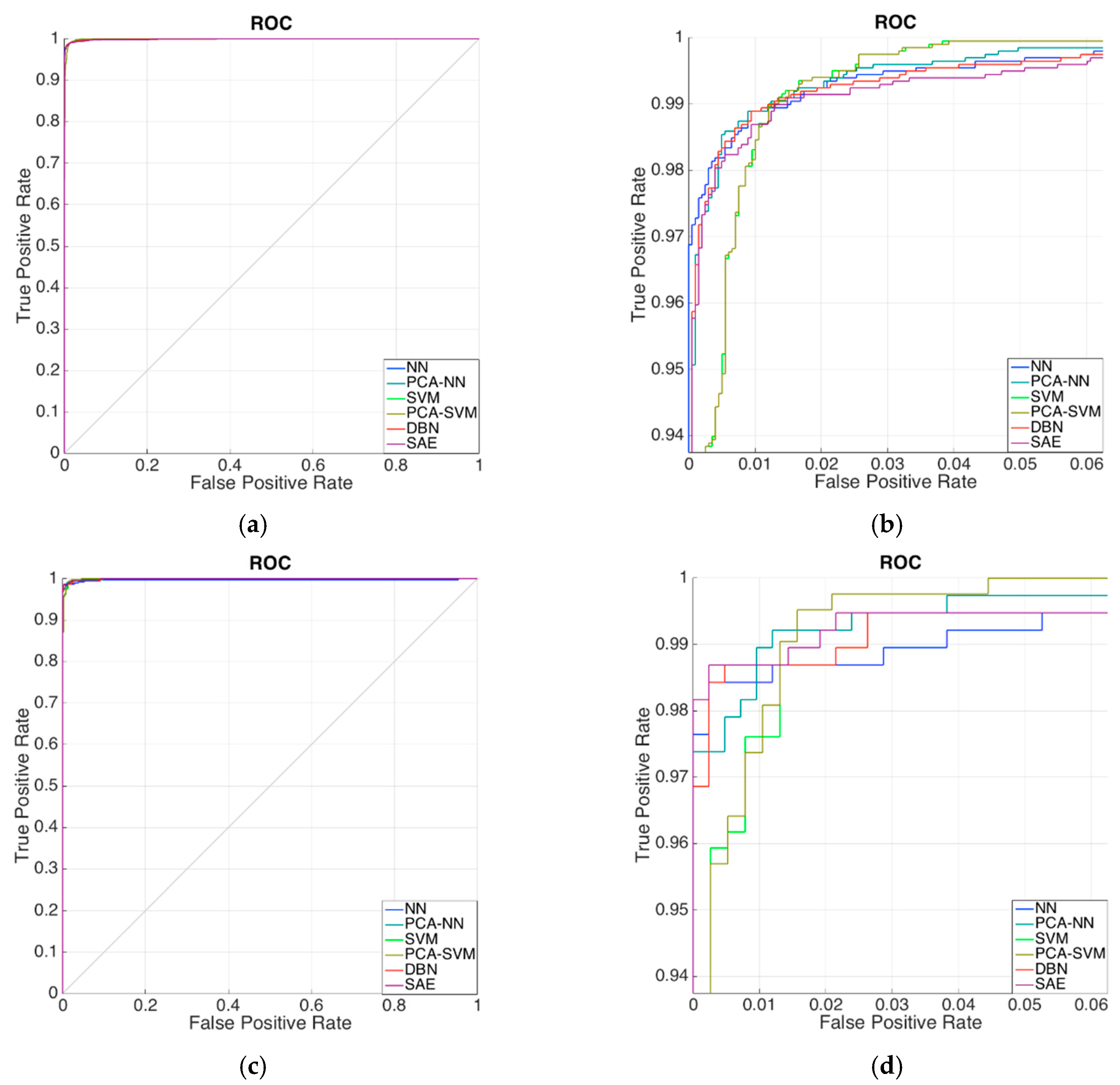
The receiver operating characteristics (ROC) of these classifiers in oil spill detection are approached based on 20,000 training, 4000 testing (Figure 8a,b) and 4000 training, 800 testing samples (Figure 8c,d) respectively. All the ROC curves are very close to the upper-left corner of the ROC map (Figure 8a,c). In the zoomed-in map (Figure 8b,d), some minor differences can be observed. Compared with other classifiers, SVM achieved a lower true positive rate under low false positive rate requirements, and higher true positive rate under high false positive rate requirements. And for NN the situation is just opposite. Deep neural networks, SAE and DBN achieved a modest true positive rate in the whole false positive rate range.
4. Conclusions
In this paper, the capability of polarimetric SAR to detect and classify marine oil spills was investigated. Potential features were extracted from a covariance matrix, a coherence matrix and a Stokes vector of the original SLC quad-pol SAR data. Deep learning algorithms together with classic classifiers were compared and analyzed. A key discovery of this paper is that given insufficient number of data samples, deep learning algorithms such as SAE and DBN can achieve better performance than traditional algorithms by initializing their parameters from a position closer to the optimum solution. Polarimetric SAR data confirmed its strong capacity in distinguishing mineral oil and its biogenic lookalikes. This can be achieved by a one-step operation, with no need to firstly segment and then classify data samples based on auxiliary information. The advantages demonstrated by polarimetric SAR can greatly boost the efficiency and accuracy of marine oil spill detection. Further studies will be conducted on features extracted from compact polarimetric SAR modes, with wider swath width, to achieve larger monitoring areas and shorter revisit times: two of the prime requirements for marine surveillance through large areas.
Acknowledgments
The RADARSAT-2 data provided by CSA and MDA is highly appreciated. This research is jointly supported by the National Key Research and Development Program of China (2016YFB0501501) and the Natural Scientific Foundation of China (41471353 and 41706201). The authors would like to thank the anonymous reviewers for their valuable comments and suggestions that helped improve the quality of this manuscript.
Author Contributions
Yu Li and Yuanzhi Zhang conceived and designed the experiments. Guandong Chen performed the experiments and analyzed the data. Yu Li, Guangmin Sun and Yuanzhi Zhang wrote the paper.
Conflicts of Interest
The authors declare no conflicts of interest.
References
- Fingas, M. The Basics of Oil Spill Cleanup; Lewis Publisher: Boca Raton, FL, USA, 2001. [Google Scholar]
- Alves, T.M.; Kokinou, E.; Zodiatis, G.; Lardner, R.; Panagiotakis, C.; Radhakrishnan, H. Modelling of oil spills in confined maritime basins: The case for early response in the Eastern Mediterranean Sea. Environ. Pollut. 2015, 206, 390–399. [Google Scholar] [CrossRef] [PubMed]
- Lardner, R.; Zodiatis, G. Modelling oil plumes from subsurface spills. Mar. Pollut. Bull. 2017. [Google Scholar] [CrossRef] [PubMed]
- Soomere, T.; Döös, K.; Lehmann, A.; Meier, H.M.; Murawski, J.; Myrberg, K.; Stanev, E. The potential of current- and wind-driven transport for environmental management of the baltic sea. Ambio 2014, 43, 94–104. [Google Scholar] [CrossRef] [PubMed] [Green Version]
- Chrastansky, A.; Callies, U. Model-based long-term reconstruction of weather-driven variations in chronic oil pollution along the German North Sea coast. Mar. Pollut. Bull. 2009, 58, 967–975. [Google Scholar] [CrossRef] [PubMed]
- Alpers, W.H.; Espedal, A. Oils and Surfactants. In Synthetic Aperture Radar Marine User’s Manual; Christopher, R.J., Apel, J.R., Eds.; US Department Commerce: Washington, DC, USA, 2004. [Google Scholar]
- Gade, M.; Alpers, W. Using ERS-2 SAR for routine observation of marine pollution in European coastal waters. Sci. Total Environ. 1999, 237, 441–448. [Google Scholar] [CrossRef]
- Ferraro, G.; Meyer-Roux, S.; Muellenhoff, O.; Pavliha, M.; Svetak, J.; Tarchi, D.; Topouzelis, K. Long term monitoring of oil spills in European seas. Int. J. Remote Sens. 2009, 30, 627–645. [Google Scholar] [CrossRef]
- Migliaccio, M.; Tranfaglia, M.; Ermakov, S.A. A physical approach for the observation of oil spills in SAR images. IEEE J. Ocean. Eng. 2005, 30, 496–507. [Google Scholar] [CrossRef]
- Topouzelis, K.; Karathanassi, V.; Pavlakis, P.; Rokos, D. Detection and discrimination between oil spills and look-alike phenomena through neural networks. ISPRS J. Photogramm. Remote Sens. 2007, 62, 264–270. [Google Scholar] [CrossRef]
- Garcia-Pineda, O.; MacDonald, I.R.; Li, X.; Jackson, C.R.; Pichel, W.G. Oil spill mapping and measurement in the gulf of Mexico with Textural Classifier Neural Network Algorithm (TCNNA). IEEE J. Sel. Top. Appl. Earth Obs. Remote Sens. 2013, 6, 2517–2525. [Google Scholar] [CrossRef]
- Pan, G.; Tang, D.; Zhang, Y. Satellite monitoring of phytoplankton in the East Mediterranean Sea after the 2006 Lebanon oil spill. Int. J. Remote Sens. 2012, 33, 7482–7490. [Google Scholar] [CrossRef]
- Solberg, A.H.S. Remote sensing of ocean oil-spill pollution. Proc. IEEE 2012, 100, 2931–2945. [Google Scholar] [CrossRef]
- Migliaccio, M.; Gambardella, A.; Tranfaglia, M. SAR polarimetry to observe oil spills. IEEE Trans. Geosci. Remote Sens. 2007, 45, 506–511. [Google Scholar] [CrossRef]
- Migliaccio, M.; Nunziata, F.; Gambardella, A. On the co-polarized phase difference for oil spill observation. Int. J. Remote Sens. 2009, 30, 1587–1602. [Google Scholar] [CrossRef]
- Nunziata, F.; Migliaccio, M.; Gambardella, A. Pedestal height for sea oil slick observation. IET Radar Sonar Navig. 2011, 5, 103–110. [Google Scholar] [CrossRef]
- Minchew, B.; Jones, C.E.; Holt, B. polarimetric analysis of backscatter from the deepwater horizon oil spill using L-band synthetic aperture radar. IEEE Trans. Geosci. Remote Sens. 2012, 50, 3812–3830. [Google Scholar] [CrossRef]
- Zhang, B.; Perrie, W.; Li, X.; Pichel, W. Mapping sea surface oil slicks using RADARSAT-2 quad-polarization SAR image. Geophys. Res. Lett. 2011, 38. [Google Scholar] [CrossRef]
- Skrunes, S.; Brekke, C.; Eltoft, T. An experimental study on oil spill characterization by multi-polarization SAR. In Proceedings of the 9th European Conference on Synthetic Aperture Radar (2012 EUSAR), Nuremberg, Germany, 23–26 April 2012; pp. 139–142. [Google Scholar]
- Shirvany, R.; Chabert, M.; Tourneret, J.-Y. Ship and oil-spill detection using the degree of polarization in linear and hybrid/compact dual-pol SAR. IEEE J. Sel. Top. Appl. Earth Obs. Remote Sens. 2012, 5, 885–892. [Google Scholar] [CrossRef] [Green Version]
- Salberg, A.-B.; Rudjord, O.; Solberg, A.H.S. Model based oil spill detection using polarimetric SAR. In Proceedings of the IEEE International Geoscience and Remote Sensing Symposium (IGARSS), Munich, Germany, 22–27 July 2012; pp. 5884–5887. [Google Scholar]
- Marghany, M. RADARSAT automatic algorithms for detecting coastal oil spill pollution. Int. J. Appl. Earth Obs. Geoinf. 2001, 3, 191–196. [Google Scholar] [CrossRef]
- Gambardella, A.; Giacinto, G.; Migliaccio, M. On the Mathematical Formulation of the SAR Oil-Spill Observation Problem. In Proceedings of the IEEE International Geoscience and Remote Sensing Symposium (IGARSS), Boston, MA, USA, 7–11 July 2008; pp. III-1382–III-1385. [Google Scholar]
- Frate, F.; Petrocchi, A.; Lichtenegger, J.; Calabresi, G. Neural networks for oil spill detection using ERS-SAR data. IEEE Trans. Geosci. Remote Sens. 2000, 38, 2282–2287. [Google Scholar] [CrossRef]
- Marghany, M. Genetic Algorithm for Oil Spill Automatic Detection from Envisat Satellite Data. In Proceedings of the Computational Science and Its Applications—ICCSA, Ho Chi Minh City, Vietnam, 24–27 June 2013; Murgante, B., Misra, S., Carlini, M., Carmelo, M.T., Nguyen, H., Taniar, D., Apduhan, B.O., Gervasi, O., Eds.; Springer: Berlin/Heidelberg, Germany, 2013; pp. 587–598. [Google Scholar]
- Li, Y.; Zhang, Y. Synthetic aperture radar oil spill detection based on morphological characteristics. Geospat. Inf. Sci. 2014, 17, 8–16. [Google Scholar] [CrossRef]
- Zhang, Y.; Li, Y.; Liang, X.S.; Tsou, J. Comparison of oil spill classifications using fully and compact polarimetric SAR images. Appl. Sci. 2017, 16, 193. [Google Scholar] [CrossRef]
- Hilton, G.; Salakhutdinov, R.R. Reducing the dimensionality of data with neural networks. Science 2006, 313, 504–507. [Google Scholar]
- Bengio, Y.; Lamblin, P.; Popovici, D.; Larochelle, H. Greedy Layer-Wise Training of Deep Networks. In Advances in Neural Information Processing Systems 19 (NIPS’06); MIT Press: Cambridge, MA, USA, 2006. [Google Scholar]
- Vergara, L.; Soriano, A.; Safont, G.; Salazar, A. On the fusion of non-independent detectors. Digit. Signal Process. 2016, 50, 24–33. [Google Scholar] [CrossRef]
- Li, Y.; LIN, H.; Chen, J.; Zhang, Y. Comparisons of circular transmit and linear receive compact polarimetric SAR features for oil slicks discrimination. J. Sens. 2015, 2015, 631561. [Google Scholar] [CrossRef]
- Li, Y.; Zhang, Y.; Chen, J.; Zhang, H. Improved compact polarimetric SAR quad-pol reconstruction algorithm for oil spill detection. IEEE Geosci. Remote Sens. Lett. 2014, 11, 1139–1142. [Google Scholar] [CrossRef]
- Chang, C.-C.; Lin, C.-J. LIBSVM: A library for support vector machines. ACM Trans. Intell. Syst. Technol. 2011, 2, 27. [Google Scholar] [CrossRef]
- Skrunes, S.; Brekke, C.; Eltoft, T. Characterization of marine surface slicks by Radarsat-2 multipolarization features. IEEE Trans. Geosci. Remote Sens. 2014, 52, 5302–5319. [Google Scholar] [CrossRef]
Figure 1.
The illustration of a Restricted Boltzmann Machine (RBM) with two hidden units and four visible units.
Figure 1.
The illustration of a Restricted Boltzmann Machine (RBM) with two hidden units and four visible units.
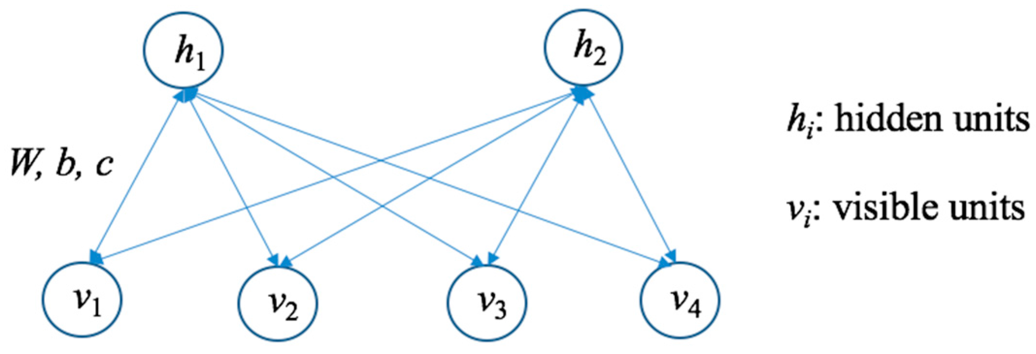
Figure 2.
The structure of an autoencoder.

Figure 3.
The demonstration of stacked autoencoder.
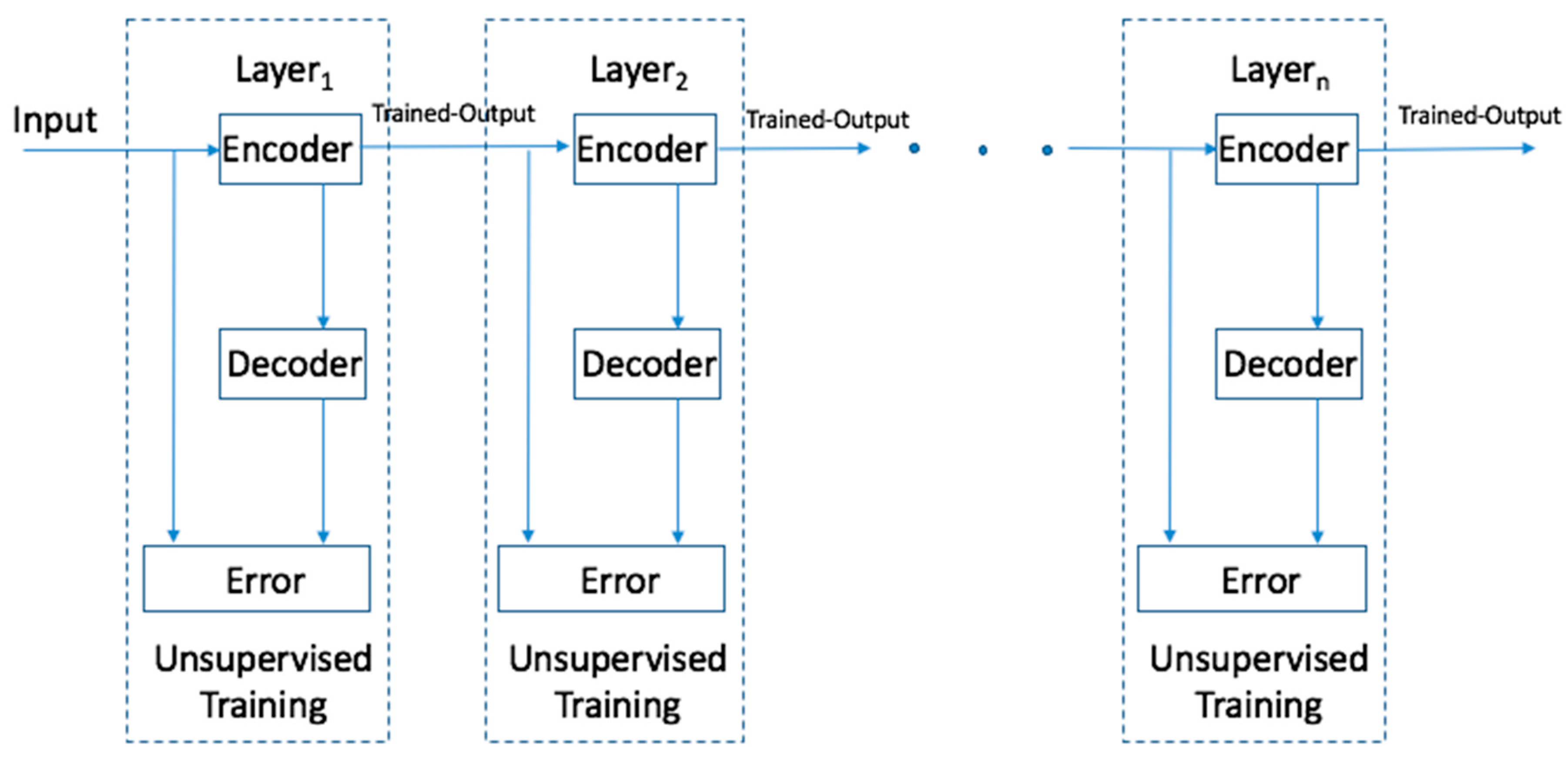
Figure 4.
Pauli RGB image of RADARSAT-2 data. (RADARSAT-2 Data and Products © Macdonald, Dettwiler and Associates Ltd., Vancouver, BC, Canada, 2011—All Rights Reserved. RADARSAT is an official mark of the Canadian Space Agency).
Figure 4.
Pauli RGB image of RADARSAT-2 data. (RADARSAT-2 Data and Products © Macdonald, Dettwiler and Associates Ltd., Vancouver, BC, Canada, 2011—All Rights Reserved. RADARSAT is an official mark of the Canadian Space Agency).
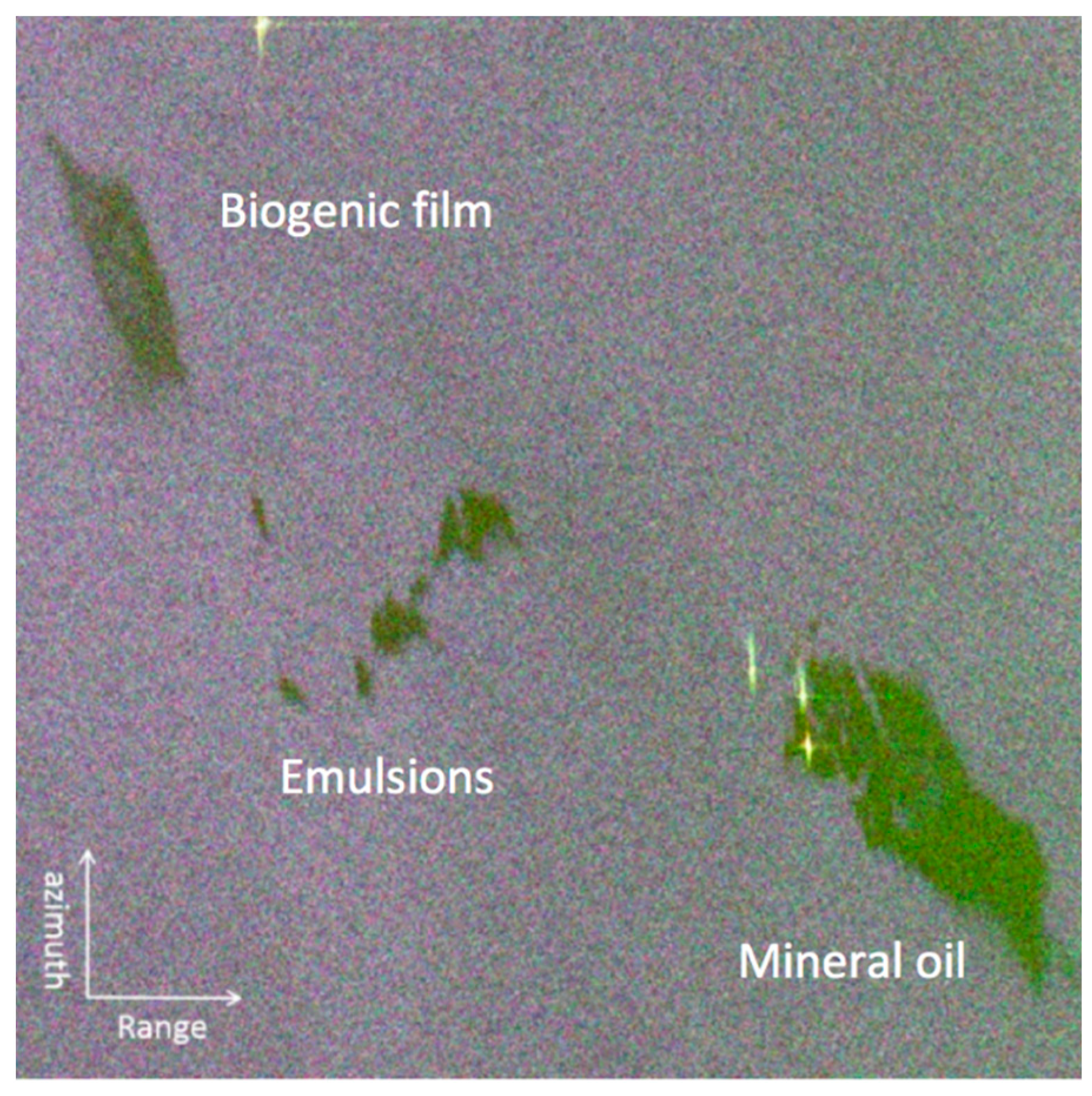
Figure 5.
Demonstration of a selected area for analysis (taking VV2 image as background); 24,000 pixels are picked as data samples.
Figure 5.
Demonstration of a selected area for analysis (taking VV2 image as background); 24,000 pixels are picked as data samples.
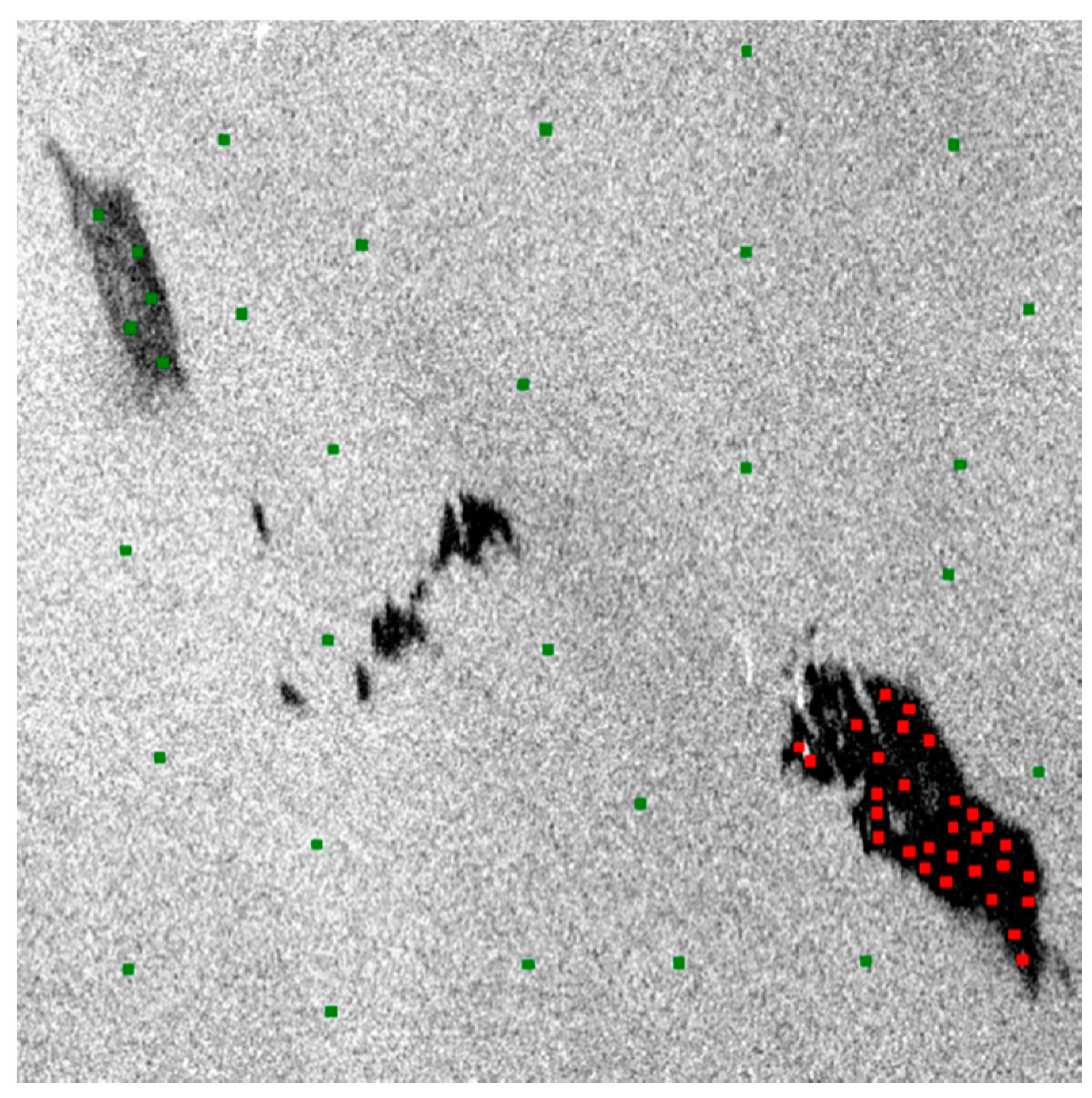
Figure 6.
Scatter plots of the main original features (a) and the features derived by principal component analysis (PCA), deep believe network (DBN) and stacked autoencoder (SAE) (b–d).
Figure 6.
Scatter plots of the main original features (a) and the features derived by principal component analysis (PCA), deep believe network (DBN) and stacked autoencoder (SAE) (b–d).

Figure 7.
Classification result achieved by SAE, 0 stands for nonoil and 1 stands for mineral oil.

Figure 8.
Receiver operating characteristics (ROC) curves of the classifiers. (a) ROC curve achieved based on 20,000 training, 4000 testing samples; (b) Zoomed in map of (a); (c) ROC curve achieved based on 4,000 training, 800 testing samples; (d) Zoomed in map of (c).
Figure 8.
Receiver operating characteristics (ROC) curves of the classifiers. (a) ROC curve achieved based on 20,000 training, 4000 testing samples; (b) Zoomed in map of (a); (c) ROC curve achieved based on 4,000 training, 800 testing samples; (d) Zoomed in map of (c).

Table 1.
Features investigated in this study.
| Feature | Definition | For Mineral Oil | For Biogenic Slicks | For Clean Sea Surface |
|---|---|---|---|---|
| VV intensity | Lower 1 | low | High | |
| Entropy (H) | High | Low | Lower | |
| Alpha (α) | High | Low | Lower | |
| Degree of Polarization (DoP) | Low | High | High | |
| Ellipticity () | Positive | Negative | Negative | |
| Pedestal Height (PH) | High | Low | Lower | |
| Standard Deviation of CPD | CPD: | High | Low | Lower |
| Conformity Coefficient (Conf. Co.) | Negative | Positive | Positive | |
| Correlation Coefficient (Corr. Co.) | Low | High | Higher | |
| Coherence Coefficient (Conf. Co.) | Low | High | Higher |
1 Note: “lower” and “higher” mean that the property of the feature on a certain type of surface is close to the other surface that has the property of “low” or “high”, but slightly lower or higher. “Std. copolarized phase difference (CPD)” stands for the standard deviation of CPD.
Table 2.
Parameter settings of the neural network.
| Parameter | Value |
|---|---|
| Sizes of layers | [10, 8, 6, 2] |
| Activation function | Sigmoid |
| Learning rate | 1 |
| Number of epochs | 100 |
| Batch size | 100 |
Table 3.
Parameter settings of the support vector machine (SVM).
| Parameter | Value |
|---|---|
| Type of SVM | C-SVC (n kind classification) |
| Type of kernel | Radial Basis Function (RBF): |
| of the RBF | 1/k (k: number of features) |
| Cost | 1 |
| (termination criterion) | 0.001 |
| Weight wi | 1 (set the parameter C of class i to wi × C) |
| Shrinking h | 1 (use the shrinking heuristics) |
Table 4.
Parameter settings of the stacked autoencoder (SAE).
| Parameter | Value |
|---|---|
| Sizes of SAE layers | [8, 6] |
| Activation function SAE | Sigmoid |
| Learning rate of SAE | 1 |
| Input Zero Masked Fraction of SAE | 0.5 |
| Number of epochs when training SAE | 10 |
| Batch size when training SAE | 100 |
| Size of the whole network | [10, 8, 6, 2] |
| Activation function of the neural network | Sigmoid |
| Learning rate when making fine-tuning | 3 |
| Number of epochs when making fine-tuning | 100 |
| Batch size when making fine-tuning | 100 |
Table 5.
Parameter settings of the deep belief network (DBN).
| Parameter | Value |
|---|---|
| Sizes of RBM layers | [8, 6] |
| Number of epochs when training RBM | 10 |
| Batch size when training RBM | 100 |
| Momentum for RBM | 0 |
| Learning rate alpha of RBM | 1 |
| Size of the whole network | [10, 8, 6, 2] |
| Activation function of the neural network | Sigmoid |
| Number of epochs when making fine-tuning | 100 |
| Batch size when making fine-tuning | 100 |
Table 6.
Testing error (1-accuracy) of classification achieved by different classifiers and on different sizes of data samples.
Table 6.
Testing error (1-accuracy) of classification achieved by different classifiers and on different sizes of data samples.
| Classifier | Number of Data Samples (Training-Testing) Accuracy (Execution Time/Seconds) | ||
|---|---|---|---|
| a. 20,000–4000 | b. 4000–800 | c. 800–160 | |
| SVM (support vector Machine) | 1.26% (1.16) | 1.38% (0.07) | 1.64% (0.01) |
| NN (nerual network) | 1.16% (6.52) | 1.68% (1.33) | 2.13% (0.34) |
| PCA (principal component analysis)-SVM | 1.20% (0.9) | 1.33% (0.06) | 1.58% (0.01) |
| PCA-NN | 1.17% (6.2) | 1.48% (1.2) | 1.90% (0.35) |
| SAE (stacked autoencoder) | 1.05% (6.33) | 1.33% (1.24) | 1.39% (0.32) |
| DBN (deep believe network) | 1.16% (5.63) | 1.42% (1.18) | 1.53% (0.28) |
Table 7.
Confusion Matrix (20,000 training, 4000 testing, six-fold) derived by SAE.
| Confusion Matrix of SAE | Mineral Oil | Non Mineral Oil | Total |
|---|---|---|---|
| Mineral oil (truth) | 11,844 | 150 | 12,000 |
| Nonmineral oil (truth) | 101 | 11,896 | 12,000 |
| Total | 11,948 | 12,052 | 24,000 |
Table 8.
DBN Confusion Matrix (20,000 training, 4000 testing, six-fold) derived by DBN.
| Confusion Matrix of DBN | Mineral Oil | Non Mineral Oil | Total |
|---|---|---|---|
| Mineral oil (truth) | 11,819 | 181 | 12,000 |
| Non mineral oil (truth) | 101 | 11,899 | 12,000 |
| Total | 11,948 | 12,052 | 24,000 |
Table 9.
SAE Confusion Matrix (20,000 training, 4000 testing, six-fold) derived by NN.
| Confusion Matrix of NN | Mineral Oil | Non Mineral Oil | Total |
|---|---|---|---|
| Mineral oil (truth) | 11,881 | 119 | 12,000 |
| Non mineral oil (truth) | 160 | 11,840 | 12,000 |
| Total | 11,948 | 12,052 | 24,000 |
Table 10.
SAE Confusion Matrix (20,000 training, 4000 testing, six-fold) derived by SVM.
| Confusion Matrix of SVM | Mineral Oil | Non Mineral Oil | Total |
|---|---|---|---|
| Mineral oil (truth) | 11,893 | 107 | 12,000 |
| Non mineral oil (truth) | 201 | 11,799 | 12,000 |
| Total | 11,948 | 12,052 | 24,000 |
© 2017 by the authors. Licensee MDPI, Basel, Switzerland. This article is an open access article distributed under the terms and conditions of the Creative Commons Attribution (CC BY) license (http://creativecommons.org/licenses/by/4.0/).
Share and Cite
MDPI and ACS Style
Chen, G.; Li, Y.; Sun, G.; Zhang, Y. Application of Deep Networks to Oil Spill Detection Using Polarimetric Synthetic Aperture Radar Images. Appl. Sci. 2017, 7, 968. https://doi.org/10.3390/app7100968
AMA Style
Chen G, Li Y, Sun G, Zhang Y. Application of Deep Networks to Oil Spill Detection Using Polarimetric Synthetic Aperture Radar Images. Applied Sciences. 2017; 7(10):968. https://doi.org/10.3390/app7100968
Chicago/Turabian StyleChen, Guandong, Yu Li, Guangmin Sun, and Yuanzhi Zhang. 2017. "Application of Deep Networks to Oil Spill Detection Using Polarimetric Synthetic Aperture Radar Images" Applied Sciences 7, no. 10: 968. https://doi.org/10.3390/app7100968
Note that from the first issue of 2016, this journal uses article numbers instead of page numbers. See further details here.