Assessing the Performance of Thermal Inertia and Hydrus Models to Estimate Surface Soil Water Content

Abstract

The knowledge of soil water content (SWC) dynamics in the upper soil layer is important for several hydrological processes. Due to the difficulty of assessing the spatial and temporal SWC dynamics in the field, some model-based approaches have been proposed during the last decade. The main objective of this work was to assess the performance of two approaches to estimate SWC in the upper soil layer under field conditions: the physically-based thermal inertia and the Hydrus model. Their validity was firstly assessed under controlled laboratory conditions. Thermal inertia was firstly validated in laboratory conditions using the transient line heat source (TLHS) method. Then, it was applied in situ to analyze the dynamics of soil thermal properties under two extreme conditions of soil-water status (well-watered and air-dry), using proximity remote-sensed data. The model performance was assessed using sensor-based measurements of soil water content acquired through frequency (FDR) and time domain reflectometry (TDR). During the laboratory experiment, the Root Mean Square Error (RMSE) was 0.02 m³ m⁻³ for the Hydrus model and 0.05 m³ m⁻³ for the TLHS model approach. On the other hand, during the in situ experiment, the temporal variability of SWCs simulated by the Hydrus model and the corresponding values measured by the TDR method evidenced good agreement (RMSE ranging between 0.01 and 0.005 m³ m⁻³). Similarly, the average of the SWCs derived from the thermal diffusion model was fairly close to those estimated by Hydrus (spatially averaged RMSE ranging between 0.03 and 0.02 m³ m⁻³).

1. Introduction

Soil water content (SWC) in the upper soil layer remarkably affects runoff generation and infiltration processes, with obvious direct consequences on water fluxes through the soil–plant–atmosphere continuum [1]. Precise evaluations of this agro-ecological variable can contribute to better estimating the dynamics of these fluxes [2]. However, accurate estimation of SWC across spatial and temporal scales is still a challenging task mainly at high temporal (minutes to days) observation scales and high spatial resolution (~0.1 m).

Even though remote sensing (RS) does not provide direct measurements of surface SWC, models employing remotely-sensed thermal and visible/near-infrared images have been developed to this aim. Thermal inertia, in particular, has already been proven to be suitable to assess the actual distribution of SWC at spatial resolutions ranging from ~1 m to ~1 km by processing airborne or satellite images [3,4]. Estimations of SWC are based on the existing relationship with soil thermal properties [3], which depends on soil bulk density, specific thermal capacity and thermal conductivity. Indeed, thermal inertia is equal to the square root of the product between volumetric heat capacity and thermal conductivity and it represents the admittance of the medium to change its temperature as a result of heat storage or release.

The accuracies of these methods, based on high-resolution remote-sensing data (acquired from a proximity platform) are still unexplored. Many authors [5,6] attempted to develop spatial information on thermal inertia distribution using the daily maximum and minimum radiative temperatures of the soil surface acquired by remote or proximity sensing. In these studies, different algorithms, usually referring to the radiative surface temperature, have been proposed to map the thermal inertia distribution [7]. Recently, other studies have shown the potential usefulness of the thermal inertia approach to estimate SWC by means of daytime and nighttime surface temperatures, as well as visible-near infrared (VIS-NIR) images [3,8,9].

Since the magnitude of the water thermal inertia is greater than that corresponding to the porous medium, the changes in the thermal inertia of soil can provide significant indications for its water content. In fact, SWC regulates the ability of soil to change its thermal status by accumulating or releasing heat within a defined time interval. Indeed, heat storage or release is forced by the energy balance at the soil surface. In particular, the amplitude of temperature variations is a direct consequence of the amount of energy entering the soil through the shortwave albedo.

Coupling between the emerging surface thermal imaging techniques [3] and hydrological physically-based models [10] could provide accurate assessment for SWC dynamics at different temporal and spatial scales. More specifically, it could be valuable to couple remote sensing and hydrological physically-based (e.g., Hydrus 2D) models to exploit their benefits: the former capable of describing the spatial patterns of SWC at the acquisition time, the latter able to describe the SWC in time usually at some points of the domain.

Hydrological physically-based models can be considered powerful and simple tools to predict SWC at various soil depths. During the last decades, a number of models have been developed and applied to simulate mass exchange processes in the soil–plant–atmosphere (SPA) continuum [11,12,13]. Several models have been proposed to simulate all the components of the water balance, including actual crop evapotranspiration [14], in particular under arid and semi-arid conditions [15,16], deep percolation [17], and water and solute transport [18,19].

The Hydrus numerical model [20], a physically-based code which solves the Richards equation for variably saturated water flow, allows simulating water and solute movement in one, two and three-dimensional variably saturated porous media. Nevertheless, using the model requires preliminary validation to assess its outcomes under site-specific conditions. Several authors have assessed the suitability of Hydrus-2D to simulate the infiltration processes of water and solutes in the soil, evidencing fairly good agreements between simulated and observed SWCs [13,21,22,23,24]. To the knowledge of the authors, there are a few continuous long-term observed SWC datasets (e.g., [25,26]), available at a very high temporal resolution, to be used for model calibration and validation. Model simulations have usually been run with daily time steps and have been compared with weekly to monthly simulation time domains.

The objective of this paper is to assess the performance of the thermal inertia and Hydrus numerical models to estimate SWC in the upper soil layer. After the detailed calibration of the empirical equation relating thermal inertia and SWC under controlled laboratory conditions (thermal inertia based on the TLHS method), a remote-sensing-based approach (thermal inertia based on proximity sensing data) was applied in situ to assess the SWC under two extreme conditions of soil-water status (well-watered and air-dry). Despite the ability of remote sensing to describe the spatial patterns, in this application the technique was used to retrieve punctual values of SWC, which were compared with those obtained by other assessment methods. Continuous, independent, sensor-based measurements of SWC (TDR measurements) allowed the evaluation, qualitatively and quantitatively, of the performance of the thermal inertia and Hydrus models.

2. Theoretical Background

2.1. Thermal Inertia

SWC represents the main soil parameter influencing the heat transfer processes involved in the soil. The thermal inertia approach is based on the solution of the first-order approximation of a one-dimensional (1-D) diffusion equation at the soil surface (z = 0) by imposing the boundary and initial conditions. The method requires the evaluation of actual soil thermal inertia, P [J m⁻² K⁻¹ s^−1/2], and the corresponding values at dry, P_dry, and wet, P_wet, conditions. When soil bulk density ρ [kg m⁻³] is known, P_dry and P_wet can be estimated by measuring the thermal conductivity, k [J m⁻¹s⁻¹ K⁻¹], and the soil specific heat, c_p [J kg⁻¹ K⁻¹]:

$$P=k\sqrt{D}=\sqrt{\rho k{c}_p}$$

(1)

where D (m² s⁻¹) is the thermal diffusivity equal to D = k (ρc_p)⁻¹. According to Lu et al., 2009 [9], SWC_Kp, can be estimated as:

$$SW{C}_{Kp}=e{\left(1-\frac{\ln Kp}{ϵ}\right)}^{-\frac{1}{\mu }}$$

(2)

where e [-] is the soil porosity, ε and μ are two parameters controlling the function shape (dependent on the quartz content in soil) and Kp is the so called “Kersten function”. Analogously to the normalized theory of the soil thermal conductivity (e.g., [27]), the Kersten function can be computed from thermal inertia according to [4]:

$$Kp=\frac{P-P_{dry}}{P_{wet}-P_{dry}}$$

(3)

The parameters ε and μ can be calibrated by means of a regression analysis between estimated and measured SWCs. Soil surface macroporosity could change due to rain falling causing mechanical disruption of aggregates and compaction [28]. Thus, inaccuracies in SWC_Kp retrievals might be related to the use of a constant value of e for scaling the $Kp$.

2.2. Thermal Inertia Evaluated Indoors via Soil Thermal Properties—The TLSH Method

The “transient line heat source” (TLSH) method was used to characterize k and c_p of the soil, and thus to compute P indoors (from now on referred as P_TLSH) according to Equation (1).

Heating phase. According to Carslaw and Jaeger (1959) [29] if a constant heat rate, q [m²s⁻³], is applied to an infinitely long and small “line” source (zero mass heater), the temperature response of the source over time, ΔT_q [K], in the transient during the heating time t_q [s] is described by:

$$\mathsf{\Delta }{T}_q=\frac{q}{4\pi kt}{E}_i\left(\frac{-r_q^2}{4Dt}\right)\mathrm{for}0<t\le t_q$$

(4a)

where k and D refer to the thermal conductivity and thermal diffusivity of the medium in which the line is buried, r_q [m] is the distance from the line at which the temperature is measured, while E_i is the exponential integral. Due to the short heating time, the redistribution of SWC due to the thermal gradient can be neglected.

Recovery phase. The temperature rise after turning off the heating source is given by:

$$\mathsf{\Delta }{T}_q=\frac{q}{4\pi kt}{E}_i\left(\frac{-r_q^2}{4Dt}\right)+\frac{q}{4\pi kt}{E}_i\left(\frac{-r_q^2}{4D\left(t-t_q\right)}\right)fort>t_q$$

(4b)

The thermal properties of the material are determined by fitting time series temperature data during heating, to the ones obtained during cooling.

Equations describing the heating (Equation (4a)), as well as the recovery (Equation (4b)) phases, cannot be explicated for D and K. The Puiseux series of E_i can be represented as a series expansion, and approximated using the first two terms as:

$$\mathsf{\Delta }{T}_q\cong \frac{q}{4\pi k}\ln \left(t\right)-\frac{q}{4\pi k}\left(\gamma +ln\left(\frac{r_q^2}{4D}\right)\right)\mathrm{for}0<t\le t_q$$

(4c)

where, γ is the Euler’s constant, and

$$\mathsf{\Delta }{T}_q\cong \frac{q}{4\pi k}\ln \left(\frac{t}{t-t_q}\right)fort>t_q$$

(4d)

This approximation is valid for large t values.

The THLS method was applied to the soil thermal properties time series acquired during a laboratory experiment to characterize the P_TLSH over the whole range of variability of SWC (see Section 3).

2.3. Thermal Inertia Evaluated In Situ via Remote-Sensing Thermal and Optical Images

Remote-sensing soil water contents, SWC_RS, can be computed by substituting a simplified thermal inertia, the so-called apparent thermal inertia, ATI* [-], in place of the actual thermal inertia, P:

$$Kp=\frac{P-P_{dry}}{P_{wet}-P_{dry}}\approx \frac{AT{I}^{*}-AT{I}_{dry}^{*}}{AT{I}_{wet}^{*}-AT{I}_{dry}^{*}}$$

(5)

The method requires two thermal images (acquired at different times), the solar irradiance reaching the ground, E₀ [W m⁻²] and the shortwave albedo at noon, α_SW [-]. The value of ATI* is computed as:

$$AT{I}^{*}=\frac{\left(1-{\alpha }_{SW}\right)}{\Delta LST}·E_0·\left[cos\left({\omega }_{t2}-{\delta }_1\right)-cos\left({\omega }_{t1}-{\delta }_1\right)\right]$$

(6)

where ∆LST = LST_t2 − LST_t1 is the land surface temperature difference between two acquisition times, t₂ and t₁, ω [s⁻¹] is the angular velocity of the earth (7.27 × 10⁻⁵ rad s⁻¹), and δ₁ [s⁻¹] is the phase difference of soil temperature for the first order approximation of the mono-dimensional thermal diffusion equation of semi-infinite homogeneous soil [3]. Equivalence in Equation (5) is valid when solar altitude and phase difference can be assumed to be almost constant in time and space. This condition occurs when the Xue and Cracknell approximation [30] is used to calculate P. Once $Kp$ is calculated, SWC_RS is computed using Equation (2).The thermal inertia method was applied to remote-sensing images acquired during a field experiment aimed to assess the SWC spatial distribution (see Section 3).

2.4. Hydrus 1D and 2D Simulation Codes

Accurate and continuous estimations of SWC dynamics can be obtained with deterministic soil-water flux models, such as those solving the Richards equation [31,32]. In this context, the Hydrus model [33] simulates the movement of water in variably saturated soil using the Richards equation, that in the mono-dimensional dimension can be written as:

$$\frac{\partial SWC}{\partial t}=\frac{\partial }{\partial x}\left[K\left(\frac{\partial h}{\partial x}+\cos \alpha \right)\right]-S$$

(7)

where h [m] is the water pressure head, SWC [m³m⁻³] is the volumetric soil water content, t [s] is time, x[m] is the spatial coordinate (positive upward), α is the angle between flow direction and the vertical axis (α = 0° for vertical flow, 90° for horizontal flow and 0° < α < 90° for the inclined flow), S [m³m⁻³ s⁻¹] is the sink term and K [ms⁻¹] is the unsaturated hydraulic conductivity function.

In order to simulate soil water movement and solute transport in two-dimensional directions, Hydrus-2D allows solving the governing equations of water movement by considering a bi-dimensional vertical plane or three dimensional regions exhibiting radial symmetry around the vertical axis. Under these conditions, Richards equation can be rewritten in its two-dimensional form as:

$$\frac{\partial SWC}{\partial t}=\frac{\partial }{\partial x_i}\left[K\left(K_{i,j}^A\frac{\partial h}{\partial x}+K_{i,j}^A\right)\right]-S$$

(8)

where, x_i and x_j [m] are the spatial coordinates, and $K_{i,j}^A$ are the components of a dimensionless anisotropy tensor K^A.

The model requires the knowledge of the soil water retention curve, SWC(h) and the hydraulic conductivity function, K(h), that can be expressed based on the van Genuchten–Mualem model [34,35]:

$$SWC=SW{C}_r+\left(SW{C}_s+SW{C}_r\right)\frac{1}{{\left[1+{\left|\alpha h\right|}^n\right]}^m}$$

(9)

$$K\left(SWC\right)=K_s{\left[\frac{\left(SWC-SW{C}_r\right)}{\left(SW{C}_s-SW{C}_r\right)}\right]}^{\lambda }{\left[1-{\left(1-{\left(\frac{\left(SWC-SW{C}_r\right)}{\left(SW{C}_s-SW{C}_r\right)}\right)}^{\frac{1}{m}}\right)}^m\right]}^2$$

(10)

where, SWC_r and SWC_s [m³ m⁻³] are the residual and saturated soil water content, K_s [m s⁻¹] is the saturated hydraulic conductivity, α [m⁻¹], n [-], m [-] and λ [-] are fitting parameters.

The sink term (S), representative of actual root water uptake (volume of soil water removed per unit of time), can be described as a fraction α_s (h) (0 ≤ α (h) ≤1) of the potential water uptake rate, S_p [m³ m⁻³ s⁻¹] [36]. Actual root water uptake is assumed to be zero, α_s (h) = 0, when the soil-water content is equal to the wilting point, whereas it is maximum, α_s (h) = 1, in the absence of crop water-stress, so that the soil water status is not limiting the plant growth [37,38].

The Hydrus model was applied to assess SWC during both a laboratory experiment and a field application (see Section 3).

3. Materials and Methods

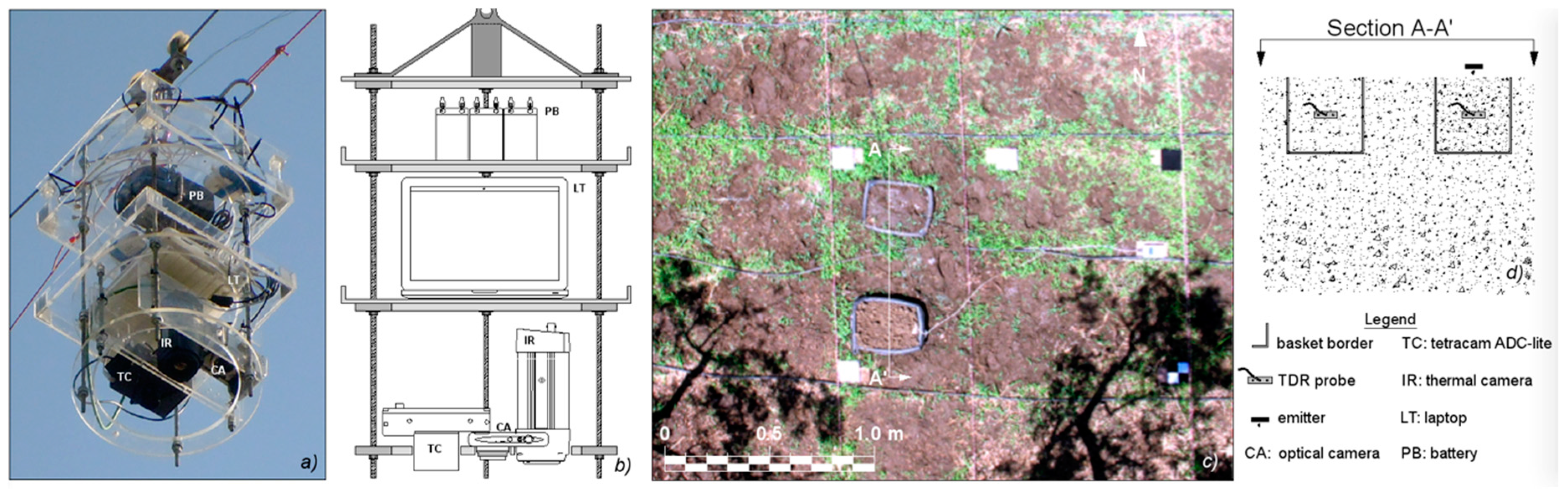
3.1. Description of Laboratory and Field Experimental Setup

A laboratory experiment was initially carried out on a disturbed soil sample (0.20 m in diameter and 0.18 m in height) filled with soil collected in the same field where the trial was implemented. The soil was oven-dried at 40 °C, sieved at 0.5 mm and then placed into a Plexiglas cylinder after sealing the bottom side. During the gradual filling of the cylinder, two KD2Pro Thermal Properties Analyzer (Decagon Devices Inc., Pullman, WA, USA) and one ML3-ThetaProbe soil moisture sensor (Delta-T device Inc., Cambridge, UK) were installed.

The commercial KD2Pro allows the evaluation of the thermal conductivity through two phases, a heating phase which lasts for 30 s, followed by a cooling phase for the subsequent 30 s.

The measurement of thermal inertia and SWC via the TLHS method and ThetaProbe respectively, allowed the calibrating of the relationship between P and SWC (Equation (2)), using only indoor data.

Once the relationship between P and SWC was retrieved, the spatial distribution of SWC was determined in situ via remote sensing, using only shortwave and thermal images. Remote-sensing-derived SWCs were then validated using independent measures.

ML3-ThetaProbe soil moisture sensors were placed vertically along the cylinder axis at 0.03 m depth. A high precision balance (model Orma-BC) with a resolution of 0.1 g was used for the continuous monitoring of the cylinder weight, whose values were registered on a data logger every thirty minutes. The sensors provided measures of SWC of a small sampling volume (≈7 × 10¹ cm³ around a central rod), whereas the precision balance provided the SWC of the whole soil sample (≈2 × 10⁵ cm³).

Both SWCs are indirect estimations: the ML3-ThetaProbe allows the conversion of the electromagnetic permittivity of the soil into SWC; the sample SWC using the balance is determined via ponderal measurement and visually estimating the height of the sample (thus the volume). Due to the different sampling volumes and soil-water content distribution within the sample some differences are expected.

However, independently of the accuracies of the two measurements, SWC obtained via ML3-ThetaProbe was used to calibrate Equation (2), as the ML3-ThetaProbe and KD2Pro sampling volumes were of the same order of magnitude (~10 cm³).

The soil sample was saturated from the bottom. After reaching a soil water content near saturation, the installed sensors started to acquire and to store the data during the subsequent drying process. After 30 days, soil drying was forced by using an air heater, until the soil sample was completely dry. Sensor based measurements of soil water content and thermal properties were collected after water re-distribution. Water and temperature re-distribution started after turning off the heater which was operated for about 10 h each day. Valid measures were assumed by restricting the analysis to temporal windows where the standard deviation of the soil temperatures, provided by KD2Pro and ML3-ThetaProbe sensors, was under an imposed threshold (0.2 °C). This also minimized differences in the SWC measures provided by the balance and the ML3-ThetaProbe.

A field experiment was also carried out in the south-west of Sicily, Italy, in an area where table and oil olives (Olea europaea L., cv. Nocellara del Belice) are the main crop. The investigated area is located at a latitude of 37°38′35″ N and longitude of 12°50′50″ E, at an elevation of 123 m a.s.l. The trees are planted on a regular grid of 8 × 5 m (250 plants/ha), with mean canopy height of about 3.7 m and a crop fraction coverage equal, on average, to 0.35. The soil is classified as sandy clay loam, according to the United States Department of Agriculture classification (USDA) [39], with an average content of clay, silt and sand of 24%, 16% and 60%. The area is characterized by a typical Mediterranean climate with moderate precipitation during the fall and winter seasons, and a very high air temperature and the absence of or limited precipitation during summer.

Hourly meteorological data (air temperature, air pressure, solar radiation, precipitation, relative humidity, soil heat fluxes and soil temperature) were acquired by an eddy covariance system, used to evaluate crop water requirements [40].

Sensor-based measurements of soil water content, as well as image acquisitions, were carried out over bare soil, between two rows of the olive orchard. The soil thermal properties assessed indoors were used. The dynamics of SWC in the topsoil was in particular investigated with two buried lysimeters (0.5 m long, 0.3 m wide and 0.3 m deep) opened only at the upper boundary and maintained under extremely different soil water contents (air-dried and fully wetted). Both lysimeters were filled carefully with the same soil extracted from the digs in which they were inserted.

3.2. Soil Physical Properties

Soil water retention curves were determined in two undisturbed soil samples, 0.08 m in diameter and 0.05 m in height, collected in the layers 0–0.3 m, in proximity of the buried lysimeters. A hanging water column apparatus was used to evaluate soil water contents corresponding to soil matric potential, h, with values ranging from −0.05 to −1.5 m. The pressure plate apparatus [41], with sieved soil samples 0.05 m in diameter and 0.01 m in height, was used to determine the soil water contents corresponding to h values of −3.37 m, −10.2 m, −30.6 m, and −153.0 m. For each undisturbed sample of dry bulk density, ρ, (kg m⁻³) was also determined, whereas porosity was calculated as e = 1 − ρ/2.65 (m³ m⁻³).

The van Genuchten model [34] was used to fit the experimental data; the water retention curve parameters were obtained by using the retention code RETention-Curve (RETC) [42]. Saturated hydraulic conductivity, K_s, was measured on the same samples used for the soil water-retention analysis, by means of a constant head permeameter, by following the Darcy assumptions.

Table 1. Soil physical properties of the layer 0–0.3 m (legend: saturated, SWC_s, and residual, SWC_r, soil water content; van Genuchten fitting parameters α, m and n; saturated hydraulic conductivity, K_s, soil bulk density, ρ, and porosity, e).

Layer	SWCs	SWCr	α	m	n	Ks	ρ	e
[m]	[m3 m−3]	[m3 m−3]	[m−1]	[-]	[-]	[m h−1]	[kg m−3]	[m3 m−3]
0-0.3	0.46	0.05	0.000114	0.20	1.25	0.167	1370	0.47

shows the soil water-retention curve parameters—bulk density, porosity and saturated hydraulic conductivity—obtained for the investigated layer.

The fitting parameters ε and μ of Equation (2) were retrieved in the laboratory through a least squares procedure, by minimizing the variance of residuals between the SWCs estimated (SWC_Kp) and measured by ML3-ThetaProbe soil moisture sensor (SWC_TP). In particular, the soil sample thermal properties (thermal diffusivity and conductivity) were measured with the KD2Pro sensor, by using the TLHS method.

3.3. Measurements of Soil Water Status

In the laboratory experiment, ancillary data for volumetric SWC used the measurements of the ML3-ThetaProbe working in the frequency domain reflectometry.

The temporal dynamic of soil water content in the field was monitored by means of the time domain reflectometry technique. In particular, a TDR-100 connected to a CR1000 data-logger allowed the acquisition, every thirty minutes, of the waveforms detected by two 0.2 m length TDR probes inserted horizontally in both the lysimeters, at about 0.1 m depth.

In order to determine the bulk electrical permittivity, the waveforms were analyzed through a subroutine written in the CR Basic language implemented into the data logger. The universal calibration equation proposed by [43] allowed the computation of volumetric water content, SWC_TDR.

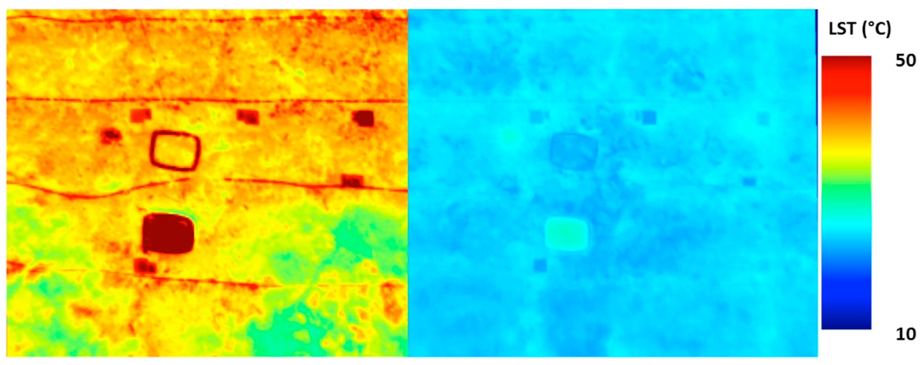
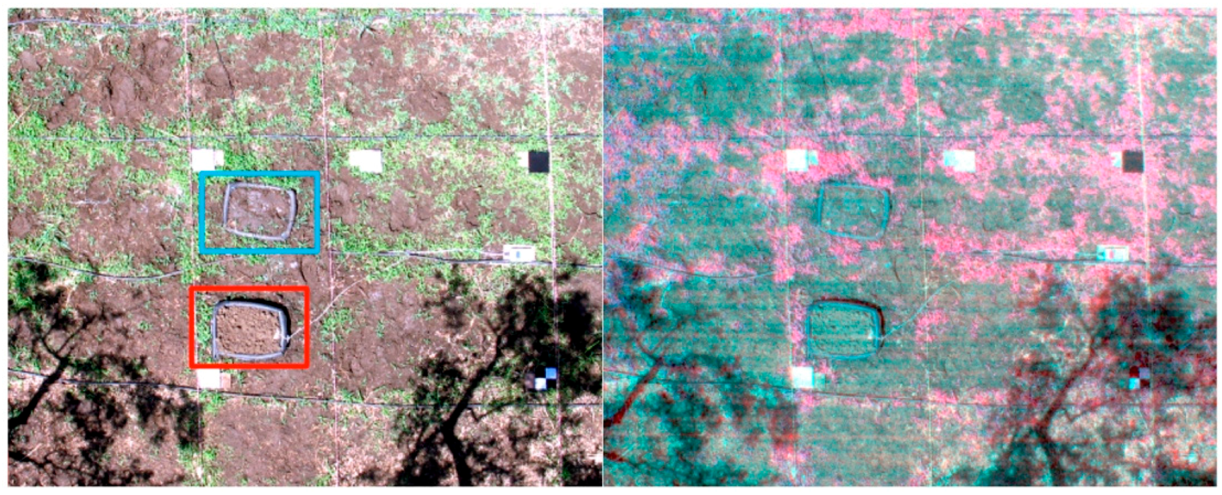
3.4. Field Image Acquisitions and Calibration

Thermal infrared (TIR) and visible-near infrared (VIS-NIR) images were acquired by a suspended platform carrying an optical PowerShotG6 digital camera (Canon Inc., Tokyo, Japan), a multispectral ADC-lite Tetracam (Tetracam Inc., Losangeles, CA, USA) and a thermal FLIR-A330 (FLIR Inc., Wilson Weil, OR, USA) camera (Figure 1a,b). Black and white reference markers were positioned to allow calibrating images by means of proximity reflectance measurements with a Field Spec Pro handled spectro-radiometer (Analytical Spectral Device, ASD, Inc., Longmont, CO, USA).

Acquisition times are listed in

Table 2. Start and end time (solar time) of the proximity sensing acquisitions.

Start Time	End Time	∆t (h)
12/7/13 05:00	12/7/13 12:59	7:59
18/7/13 13:32	18/7/13 16:37	3:05
30/7/13 13:21	30/7/13 20:00	6:39

. The thermal images from 12 July were acquired during the increasing thermal transient, whereas the images on the 18th and 30th were acquired during the decreasing thermal transient (after midday). The value of albedo (α_SW), obtained by processing shortwave reflectances, was interpolated in order to estimate its noontime value.

A number of radiometric temperature and spectro-radiometric measurements were acquired on artificial surfaces (e.g., black and white panels). The shortwave images were calibrated to spectral reflectance and corrected for atmospheric influence by applying the empirical line method, which required ground reflectance measurements over artificial targets taken simultaneously with the images [44]. The thermal images were converted into surface radiometric temperatures by means of a linear regression with in situ temperature measurements using emissivity maps of bare soil. The soil emissivity was inferred by linearly rescaling the day–night temperature variations between a minimum and a maximum value. Minimum and maximum emissivity were assumed about 0.94 (for dry soil) and 0.97 (for wet soil), respectively, as indicated by [45] for compacted sandy loam soil. Radiometric calibration was validated on natural surfaces with homogeneous radiometric characteristics (bare soils).

3.5. Hydrus Model Parametrization

The Hydrus-2D model was applied to simulate the distribution of soil water content in the soil lysimeter used for the laboratory experiment. As described above, the lysimeter was placed on the balance, to measure daily soil evaporation. The experiment was carried out from 28 September to 2 November 2016; during the first period (28 September–9 October) the lateral area of the soil cylinder was coiled by the plastic container and only the upper side was opened. Then, the plastic container was removed and a fan heater was placed 0.1 m away from the soil cylinder to accelerate the drying process. In order to account for the different boundary conditions, two simulations were run, by considering a simulation domain of 0.2 m width and 0.18 m depth. The first was carried out by assuming atmospheric conditions at the soil surface and the absence of flux along the other boundary surfaces. In the second simulation it was assumed that the evaporative surface corresponded to the upper soil surface and the lateral area of the soil cylinder.

The daily evaporation rate was calculated as the difference between the two consecutive records of weight divided by the evaporative area.

The initial soil water content was assumed constant and equal to 0.46 m³ m⁻³ (corresponding to saturation), whereas in the second simulation, the distribution of SWC obtained at the end of the previous simulation was taken into consideration. Table 1 indicates the van Genuchen–Mualem model parameters assumed for the soil hydraulic functions.

In the field experiment, both the examined conditions (dry and wet) were schematized according to a 0.30 m depth simulation domain, by assuming one-dimensional infiltration and redistribution processes along a vertical plan. A constant flux of 0.53 m h⁻¹, was obtained by dividing the emitter flow discharge by the surface of the container, was considered at the upper boundary surface during wetting events, whereas the absence of flux was considered during the redistribution process following each watering. Atmospheric conditions were therefore assumed at the soil surface, as well as the absence of flux along the lateral sides and the bottom of the simulation domain.

Simulations were run from 11 to 31 July 2013 and the initial soil water content within the soil profile was assumed to be linearly variable between 0.33 m³ m⁻³ and 0.37 m³ m⁻³ (wet) and between 0.03 m³ m⁻³ and 0.04 m³ m⁻³ (dry), based on the values measured at the beginning of the experiment. Even in this case, the van Genuchen–Mualem model was assumed to represent the soil hydraulic functions.

3.6. Statistical Analysis for Model Evaluation

The model performance was evaluated based on the root mean square error (RMSE) and the Nash–Sutcliffe efficiency coefficient [46], defined as:

$$RMSE=\sqrt{\frac{{\displaystyle {\displaystyle \sum _{i=1}^N\left(X_{sim,i}-X_{obs,i}\right)}}}{N}}$$

(11)

where N is the number of measured data, and X_sim,i and X_obs,i are the predicted and measured values of any considered variable [47].

$$E=1-\frac{{\displaystyle \sum _{i=1}^N{\left(X_{sim,i}-X_{obs,i}\right)}^2}}{{\displaystyle \sum _{i=1}^N{\left(X_{sim,i}-\overline{X_{obs}}\right)}^2}}$$

(12)

A perfect match between simulated and observed data is represented by E = 1, whereas for E = 0 the model prediction has the same accuracy as the measured mean; values of the efficiency coefficient lower than 0 indicate that the mean of measured values is a better predictor than the investigated model.

4. Results

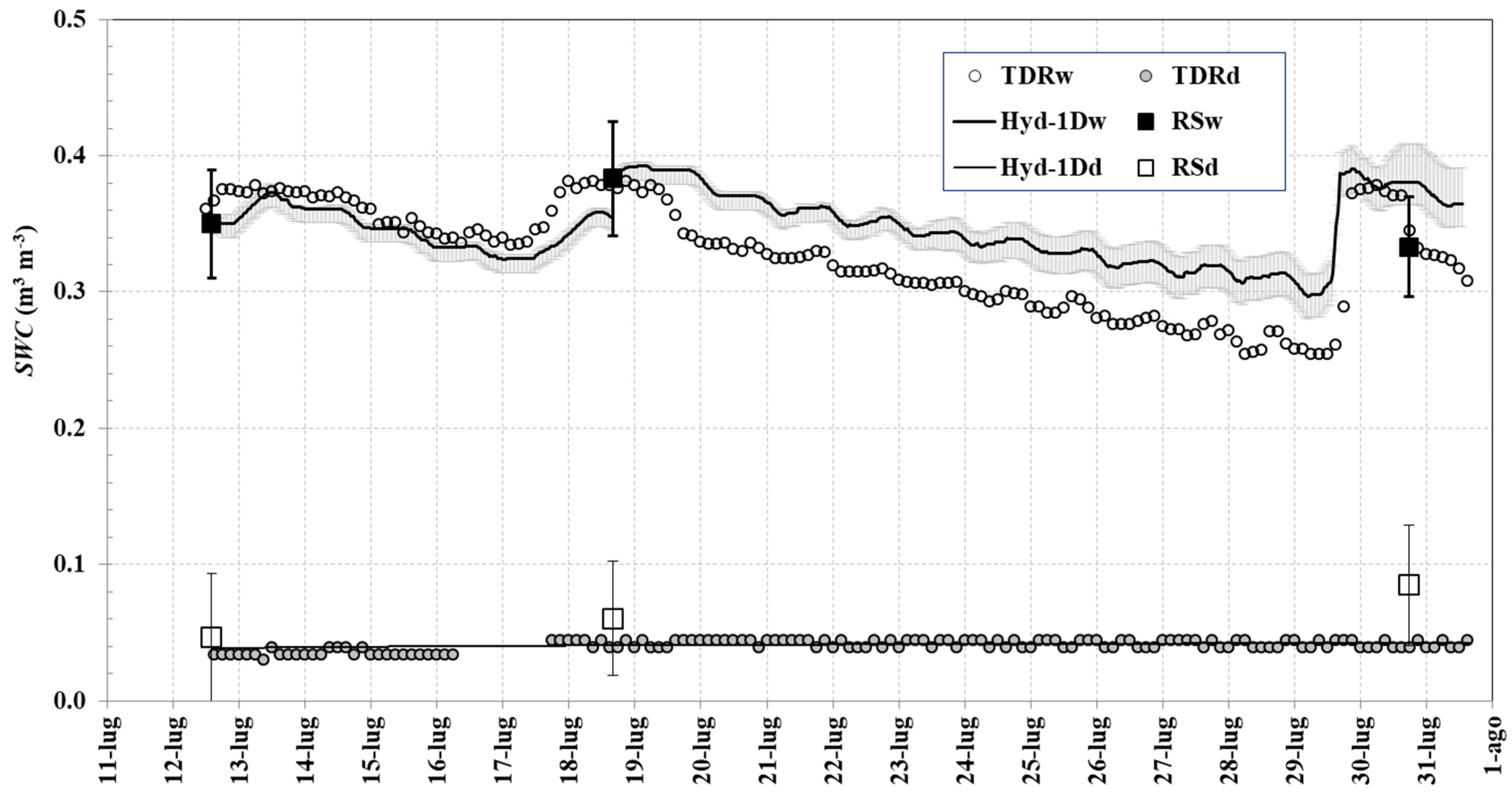
4.1. Calibration of Thermal Inertia Based on TLHS under Controlled Conditions—The Indoor Experiment

Estimation of soil water content, SWC_Kp, requires investigating the temporal variability of soil thermal properties, as well as to parameterize the model shown in Equation (2).

Soil bulk density, ρ, measured at the dry condition was about 1330 kg m⁻³, whereas the porosity, e, was estimated in about 0.5 m³ m⁻³. These values were comparable to those obtained in the field (Table 1).

Measurements of actual SWC through the ML3-ThetaProbe, SWC_TP, allowed calibrating Equation (2). The least square fitting method, by fixing e to the reported value, allowed estimating ε = 1.78 and μ = 0.47. These parameters were fitted through a generalized reduced gradient (GRG) non-linear solving method by maximizing r² and minimizing the mean absolute error (MAE). Figure 2 shows the relationship between the thermal-inertia-based soil water content, SWC_Kp, and the corresponding soil water content measured by the ML3-ThetaProbe, SWC_TP. Metrics of SWC_Kp vs. SWC_TP highlight good agreement (R² > 0.99, MAE = 0.01 m³ m⁻³, RMSE = 0.02 m³ m⁻³); however, a moderate intercept value of ~−0.03 m³ m⁻³ evidences a systematic underestimation of SWC_Kp.

Simulations of SWC temporal dynamics were also performed by the Hydrus-2Dmodel according to the schematization described in paragraph 3.5. Soil water contents simulated by Hydrus-2D (SWC_H2D) are plotted in Figure 3 together with those measured by both the balance (SWC_m) and ML3-ThetaProbe (SWC_TP). Additionally, the soil water contents estimated by the thermal inertia approach (SWC_Kp) are also shown.

A qualitative analysis of Figure 3 shows good performance of the Hydrus-2Dmodel if compared to the measured soil water content, SWC_m and SWC_TP. On the contrary, the thermal inertia model simulates values of SWCs lower than the corresponding measured ones, even if with a similar trend.

Statistically, the RMSE associated to both the models (Hydrus-2D, TLHS) were appreciable and equal to RMSE = 0.02 m³ m⁻³ for the Hydrus model and RMSE = 0.05 m³ m⁻³ for the TLHS approaches. With reference to the model efficiency, E, more than satisfactory behavior has been observed for both the Hydrus-2D (E = 0.98) and TLHS (E = 0.82) models, which can therefore be considered suitable to predict the temporal dynamic of SWC in the surface soil layer.

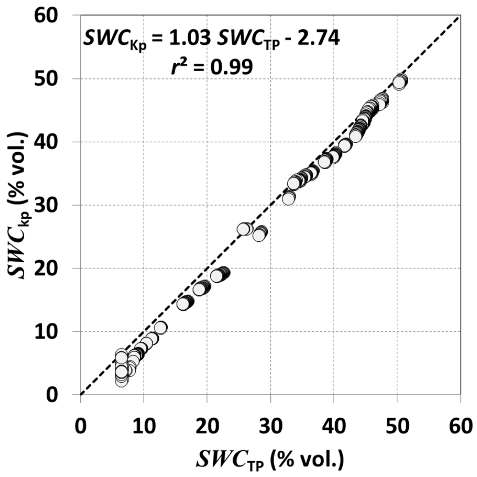
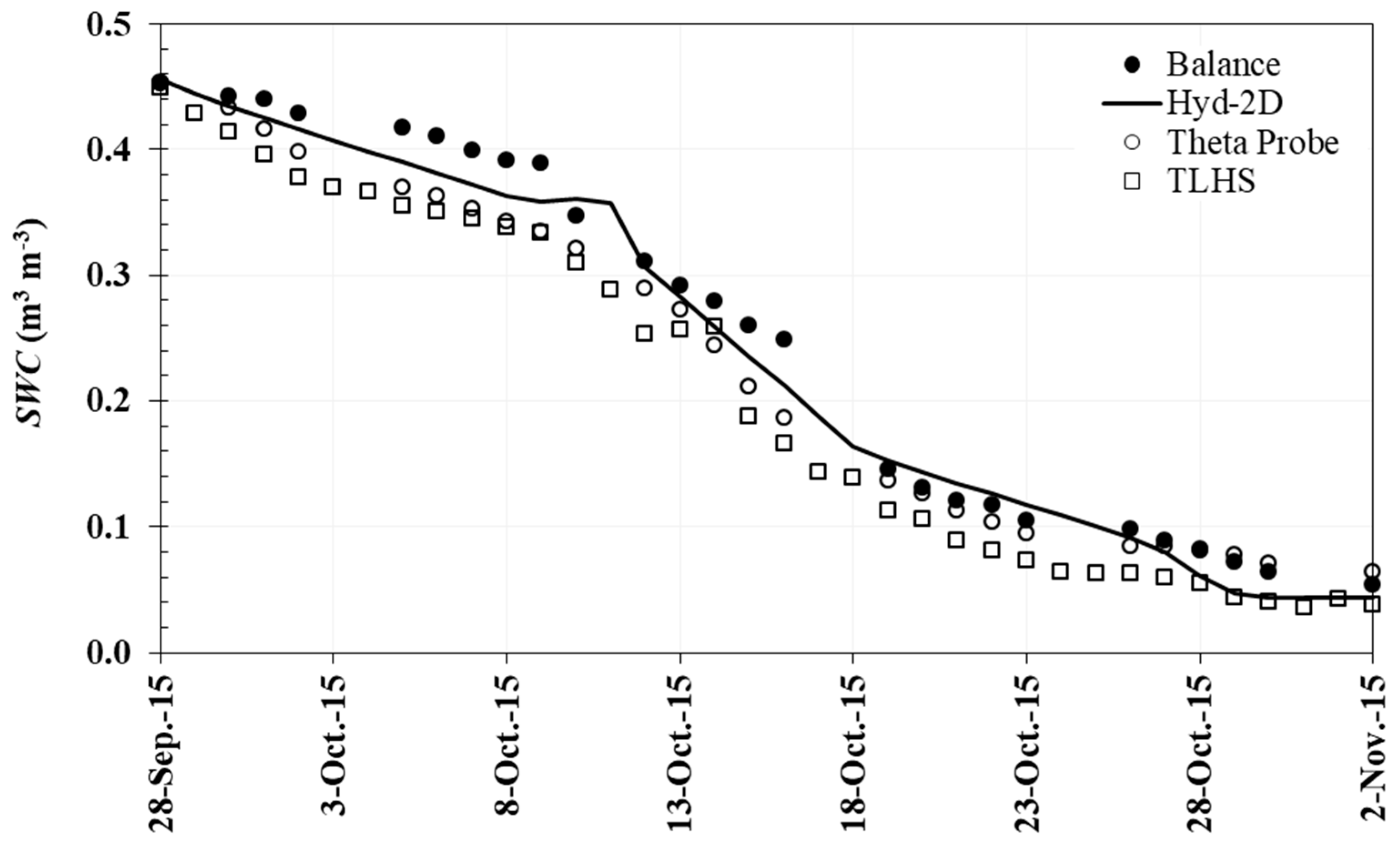
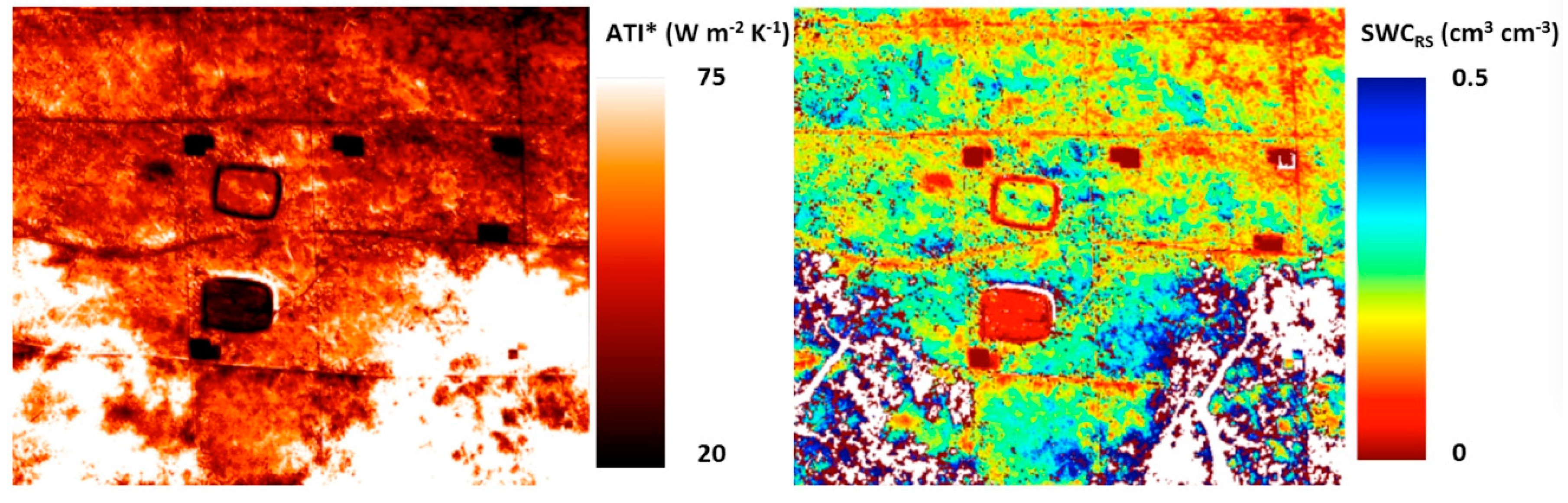
4.2. Application of Thermal Inertia Based on Proximity Sensing Images under Natural Conditions—The Field Experiment

With reference to a typical acquisition date (30 July), Figure 4 shows a true color composite image (left panel) and a color-infrared composite image (right panel) acquired at 13:21 (solar time) with the optical and the multispectral cameras, respectively. Vegetation cover is distinguishable by the reddish color (near infrared) in the color-infrared composite image.

The very high spatial resolution (~0.03 m) of the proximity-sensing images pointed out some operational limits due to the shadows of trees and soil vegetation cover.

The deployment of black and white reference targets (Figure 4) allowed the accurate in-reflectance calibration of the VIS/NIR images and thus of the albedo, α_SW. Bare soil is, on average, characterized by a lower α_SW than soil covered by vegetation, while wet soil was slightly darker than dry soil (higher α_SW). Images were characterized by the shadows of trees moving within the scene during the field acquisition that partially extinguish the incident irradiance reaching the soil; thus, we assumed reliable values of α_SW only over sunlit areas. Shadowed areas were identified through a K-means algorithm [48] and removed from the further calculations.

Figure 5 shows two thermal images (pseudo color composite) acquired at 13:21 (left panel) and 18:34 (right panel) solar time. Thermal and VIS/NIR images allowed the assessment of spatial distributions of $Kp$ (Equation (5)), and thus the remote assessment of SWC values, SWC_RS.

Daytime thermographs were characterized by high spatial variability, whereas the homogeneity of the thermal images increased between sunset and sunrise (night-time images). At night, the vegetation exhibited a higher temperature than the surrounding bare soil, while the dry basket exhibited higher temperatures than the wet one both during the day and at night.

Bare soil was, on average, characterized by a lower albedo than the soil covered by vegetation. Moreover, wet soil was slightly darker than dry soil. As expected, the white and black reference markers exhibited the extreme values (the highest and lowest albedos). The irradiance dropping during the daytime, due to the orchard olive trees, affected the sensed albedo; thus, the estimated noon albedo spatial distribution had reliable values out of shaded areas. These latter pixels were removed in SWC elaborations (Figure 6, right panel), by classifying optical and multispectral images through a K-means algorithm.

The ATI* spatial distribution shown in Figure 6 (right panel), retrieved according to Equation (6), is considered a proxy variable of the actual SWC (Figure 6, left panel): the lower the ATI*, the lower the SWC (see dry basket). The tree canopy within the scene exhibited high ATI* values. Although the model was not able to retrieve the SWC below dense vegetation [49], vegetated pixels were not removed from the image to highlight their outlier behavior. The final Remote-sensing soil water contents were masked through a Boolean operator (based on the K-means classification) to remove shadowed pixels or covered by vegetation.

On the other hand, the simulations of soil water content in two plastic baskets were performed using the one-dimensional physically-based model Hydrus-1D. Figure 7 shows the temporal dynamic of SWC simulated by Hydrus-1D (SWC_H1D) and the measurements acquired by TDR sensors in both the dry (TDR_d) and wet (TDR_w) baskets. Moreover, SWCs estimated for the three acquisition days (Table 2) by means of the RS-based TLHS model (SWC_RS) are also shown.

Analysis of the data showed the good performance of the Hydrus-1Dmodel if compared to the measured soil water contents, SWC_TDR, with RMSE values equal to 0.01 and 0.005 m³ m⁻³ respectively for the wet and the dry conditions. However, with reference to the model efficiency, E, good performance can be ascertained only in wet conditions (E = 0.98). Due to the low variability of SWC under dry conditions, the value of E was lower than zero (E = −3.25), so that the mean of the measured values is a better predictor than the considered model.

With reference to SWC predicted through the RS-based model (SWC_RS), the values were averaged over a circular area (diameter: 15 cm) to avoid the pixels close to the basket bounds and to reduce inaccuracies caused by micro-relief having an average size comparable to the spatial resolution. Micro-relief, indeed, caused small shadows un-correlated with SWC.

The error band refers to the absolute error between SWC_Kp and SWC_TP (retrieved within the indoor experiment) for a given value of SWC_Kp, thus, high spatial resolution effects on the retrieved SWC accuracy, such micro-relief effects on optical and thermal images, are not considered. Even if the field experiment has a few remote observations, it is possible to quantify good predictability using the Hydrus-1D model with an average error of RMSE equal to 0.03 and 0.02 m³ m⁻³, respectively, for wet and dry conditions.

5. Conclusions

In this paper, the performance of the thermal inertia and Hydrus models to estimate the SWC of the upper soil layer were assessed under both laboratory and field conditions. The TLSH and ThetaProbe indoor measures allowed the calibration of a relationship between soil thermal inertia and its water content. In the laboratory, the soil water content (SWC_Kp) was computed according to Lu et al.’s 2009 [8] model in which the fitting parameter, obtained by fixing the soil porosity e = 0.5 m³ m⁻³, was equal to ε = 1.78 and μ = 0.47.

A quantitative analysis of the examined models showed good performance for the Hydrus-2D model if compared to the measured soil water content, while the thermal inertia model simulated SWC values lower than those measured. However, the Nash–Sutcliffe efficiency coefficient was appreciable for both the Hydrus-2D (E = 0.98) and the thermal inertia model based on TLHS (E = 0.82), showing that both the methodologies can be considered suitable to predict the temporal dynamics of SWC in the surface soil layer.

A remote-sensing-based thermal inertia method was then applied in the open field under natural conditions, allowing monitoring of the soil thermal properties of two extreme soil water statuses (well-watered and air-dry). Continuous sensor-based measurements of the soil water content allowed the evaluation, qualitatively and quantitatively, of the performance of thermal inertia and the Hydrus-1D models.

In the field trial, the very high spatial resolution (≈0.03 m) of the proximity sensing images allowed the emphasis of the main operational limits due to tree shadows and soil vegetation cover.

On the other hand, simulations with the Hydrus-1D model allowed enhancing SWC simulated by the remote-sensing-based thermal inertia model (SWC_RS). The Hydrus-1D model showed good performance if compared to the soil water content measured by means of the TDR probe. Based on the Nash–Sutcliffe efficiency coefficient, however, the confirmation of the good performance can be ascertained only in the wet conditions (E = 0.98), being E < 0 under the dry conditions.

With reference to the RS-based model, even if a limited number of remote observations were available, it was possible to quantify good predictability with the Hydrus 1D model with average RMSEs equal to 0.03 m³ m⁻³ and 0.02 m³ m⁻³, respectively, for the wet and dry conditions.

Further investigations will be carried out to assimilate the remote sensed acquisitions in numerical models, as well as to extend the proposed application to larger scales.

References

1. Campbell, G.S.; Norman, J.M. The description and measurement of plant canopy structure. In Plant Canopies: Their Growth, Form and Function; Society for Experimental Biology, Seminar Series 29; Russell, G., Marshall, B., Jarvis, P.G., Eds.; Cambridge University Press: Cambridge, UK, 1988; pp. 1–19. [Google Scholar]
2. Vereecken, H.; Huisman, J.A.; Bogena, H.; Vanderborght, J.; Vrugt, J.A.; Hopmans, J.W. On the value of soil moisture measurements in vadose zone hydrology: A review. Water Resour. Res. 2008, 44, W00D06. [Google Scholar] [CrossRef]
3. Maltese, A.; Bates, P.D.; Capodici, F.; Cannarozzo, M.; Ciraolo, G.; La Loggia, G. Critical analysis of thermal inertia approaches for surface soil water content retrieval. Hydrol. Sci. J. 2013, 58, 1144–1161. [Google Scholar] [CrossRef]
4. Maltese, A.; Capodici, F.; Ciraolo, G.; La Loggia, G. Mapping soil water content under sparse vegetation and changeable sky conditions: Comparison of two thermal inertia approaches. J. Appl. Remote Sens. 2013, 7, 073548-1–073548-17. [Google Scholar] [CrossRef]
5. Price, J.C. Thermal inertia mapping: A new view of the Earth. J. Geophys. Res. 1977, 82, 2582–2590. [Google Scholar] [CrossRef]
6. Minacapilli, M.; Cammalleri, C.; Ciraolo, G.; D’Asaro, F.; Iovino, M.; Maltese, A. Thermal inertia modelling for soil surface water content estimation: A laboratory experiment. Soil Phys. 2012, 76, 1–9. [Google Scholar]
7. Sobrino, J.A.; El Kharraz, M.H. Combing afternoon and morning NOAA satellites for thermal inertia estimation: 2. Methodology and application. J. Geophys. Res. 1999, 104, 9455–9465. [Google Scholar] [CrossRef]
8. Minacapilli, M.; Iovino, M.; Blanda, F. High resolution remote estimation of soil surface water content by a thermal inertia approach. J. Hydrol. 2009, 379, 229–238. [Google Scholar] [CrossRef]
9. Lu, S.; Ju, Z.; Ren, T.; Horton, R. A general approach to estimate soil water content from thermal inertia. Agric. For. Meteorol. 2009, 149, 1693–1698. [Google Scholar] [CrossRef]
10. Bogena, H.R.; Huismana, J.A.; Meierb, H.; Rosenbauma, U.; Weuthena, A. Hybrid wireless underground sensor networks: Quantification of signal attenuation in soil. Vadose Zone J. 2009, 8, 755–761. [Google Scholar] [CrossRef]
11. Feddes, R.A.; Bresler, E.; Neuman, S.P. Field test of a modified numerical model for water uptake by root systems. Water Resour. Res. 1974, 10, 1199–1206. [Google Scholar] [CrossRef]
12. Bastiaanssen, W.G.M.; Allen, R.G.; Droogers, P.; D’Urso, G.; Steduto, P. Review: Twenty-Five years modeling irrigated and drained soils: State of the art. Agric. Water Manag. 2007, 92, 111–125. [Google Scholar] [CrossRef]
13. Rallo, G.; Provenzano, G. Modelling eco-physiological response of table olive trees (Olea europaea L.) to soil water deficit conditions. Agric. Water Manag. 2013, 120, 79–88. [Google Scholar] [CrossRef] [Green Version]
14. Negm, A.; Falocchi, M.; Barontini, S.; Bacchi, B.; Ranzi, R. Assessment of the waterbalance in an alpine climate: Setup of a micrometeorological station and preliminary results. Procedia Environ. Sci. 2013, 19, 275–284. [Google Scholar] [CrossRef]
15. Barontini, S.; Boselli, V.; Louki1, A.; Ben Slima, Z.; Ghaouch, F.E.; Labaran, R.; Raffelli, G.; Peli, M.; Al Ani, A.M.; Vitale, N.; et al. Bridging Mediterranean cultures in the International Year of Soils 2015: A documentary exhibition on irrigation techniques in water scarcity conditions. Hydrol. Res. 2017, 48, 789–801. [Google Scholar] [CrossRef]
16. Negm, A.; Jabro, J.; Provenzano, G. Assessing the suitability of American National Aeronautics and Space Administration (NASA) agro-climatology archive to predict daily meteorological variables and reference evapotranspiration in Sicily, Italy. Agric. For. Meteorol. 2017, 244–245, 111–121. [Google Scholar] [CrossRef]
17. Jaber, F.; Shukla, S.; Srivastava, S. Recharge, upflux and watertable response for shallow water table conditions in southwest Florida. Hydrol. Process. 2006, 20, 1895–1907. [Google Scholar] [CrossRef]
18. Van Dam, J.C.; Huygen, J.; Wesseling, J.G.; Feddes, R.A.; Kabat, P.; van Valsum, P.E.V.; Groenendijk, P.; van Diepen, C.A. Theory of SWAP, Version 2.0. Simulation of Water Flow, Solute Transport and Plant Growth in the Soil–Water–Atmosphere–Plant Environment; Department of Water Resources, WAU, Report 71; DLO Winand Staring Centre: Wageningen, The Netherlands, 1997. [Google Scholar]
19. Ragab, R.; Prudhomme, C. Climate change and water resources management in arid and semi-arid regions: Prospective and challenges for the 21st century. Biosyst. Eng. 2002, 81, 3–34. [Google Scholar] [CrossRef]
20. Šimůnek, J.; van Genuchten, M.T.; Šejna, M. The HYDRUS Software Package for Simulating Two- and Three-Dimensional Movement of Water, Heat, and Multiple Solutes in Variably-Saturated Media: Technical Manual, version 1.0; PC-Progress: Prague, Czech Republic, 2006. [Google Scholar]
21. Zappa, M.; Gurtz, J. Simulation of soil moisture and evapotranspiration in a soil profile during the 1999 MAP-Riviera Campaign. Hydrol. Earth Syst. Sci. 2003, 7, 903–919. [Google Scholar] [CrossRef]
22. Provenzano, G. Using Hydrus-2D Simulation Model to Evaluate Wetted Soil Volume in Subsurface Drip Irrigation Systems. J. Irrig. Drain. Eng. 2007, 133, 342–349. [Google Scholar] [CrossRef]
23. Roberts, T.; Lazarovitch, N.; Warrick, A.W.; Thompson, T.L. Modeling salt accumulation with subsurface drip irrigation using Hydrus-2D. Soil Sci. Soc. Am. J. 2009, 73, 233–240. [Google Scholar] [CrossRef]
24. Mguidiche, A.; Provenzano, G.; Douh, B.; Khila, S.; Rallo, G.; Boujelben, A. Assessing hydrus-2D to simulate soil water content (SWC) and salt accumulation under an SDI system: Application to a potato crop in a semi-arid area of Central Tunisia (2015). Irrig. Drain. 2013, 64, 263–274. [Google Scholar] [CrossRef]
25. Capodici, F.; Maltese, A.; Ciraolo, G.; D’Urso, G.; La Loggia, G. Power Sensitivity Analysis of Multi-Frequency, Multi-Polarized, Multi-Temporal SAR Data for Soil-Vegetation System Variables Characterization. Remote Sens. 2017, 9, 677. [Google Scholar] [CrossRef]
26. Maltese, A.; Minacapilli, M.; Cammalleri, C.; Ciraolo, G.; D’Asaro, F. A thermal inertia model for soil water content retrieval using thermal and multispectral images. In Proceedings of the SPIE—The International Society for Optical Engineering, Toulouse, France, 22 October 2010; Volume 7824. [Google Scholar]
27. Lu, S.; Ren, T.S.; Gong, Y.S.; Horton, R. An improved model for predicting soil thermal conductivity from water content at room temperature. Soil Sci. Soc. Am. J. 2007, 71, 8–14. [Google Scholar] [CrossRef]
28. Rousseva, S.; Torri, D.; Pagliai, M. Effect of rain on the macroporosity at the soil surface. Eur. J. Soil Sci. 2002, 53, 83–94. [Google Scholar] [CrossRef]
29. Carslaw, H.S.; Jaeger, J.C. Conduction of Heat in Solids, 2nd ed.; American Society of Agronomy: Oxford, UK; London, UK, 1959. [Google Scholar]
30. Xue, Y.; Cracknell, A.P. Advanced thermal inertia modelling. Int. J. Remote Sens. 1995, 16, 431–446. [Google Scholar] [CrossRef]
31. Manzini, G.; Ferraris, S. Mass conservative finite volume methods on 2–D unstructured grids for the Richards’ equation. Adv. Water Resour. 2004, 27, 1199–1215. [Google Scholar] [CrossRef]
32. Selle, B.; Minasny, B.; Bethune, M.; Thayalakumaran, T.; Chandra, S. Applicability of Richards’ equation model to predict deep percolation under surface irrigation. Geoderma 2011, 160, 569–578. [Google Scholar] [CrossRef]
33. Šimůnek, J.; Šejna, M.; van Genuchten, M.T. The HYDRUS-1D Software Package for Simulating the Onedimensional Movement of Water, Heat, and Multiple Solutes in Variably Saturated Media, version 1.0; IGWMC-TPS-70; Colorado School of Mines, International Ground Water Modeling Center: Golden, CO, USA, 1998. [Google Scholar]
34. Van Genuchten, M.T. A closed–form equation for predicting the hydraulic conductivity of unsaturated soils. Soil Sci. Soc. Am. J. 1980, 44, 892–898. [Google Scholar] [CrossRef]
35. Mualem, Y. A new model for predicting the hydraulic conductivity of unsaturated porous media. Water Resour. Res. 1976, 12, 513–522. [Google Scholar] [CrossRef]
36. Feddes, R.A.; Kowalik, P.J.; Zaradny, H. Simulation of Field Water Use and Crop Yield; Simulation Monographs; Pudoc: Wageningen, The Netherlands, 1978; 188p. [Google Scholar]
37. Feddes, R.A.; Hoff, H.; Bruen, M.; Dawson, T.; DeRosnay, P.; Dirmeyer, P.; Jackson, R.B.; Kabat, P.; Kleidon, A.; Lilly, A.; et al. Modeling root water uptake in hydrological and climate models. Bull. Am. Meteorol. Soc. 2001, 82, 2797–2809. [Google Scholar] [CrossRef]
38. Šimůnek, J.; van Genuchten, M.T. Modelling nonequilibrium flow and transport with HYDRUS. Vadose Zone J. 2008, 7, 782–797. [Google Scholar] [CrossRef]
39. Gee, G.W.; Or, D. Particle-size analysis. In Methods of Soil Analysis. Part. 4. Physical Methods, 3rd ed.; Dane, J.H., Topp, G.C., Eds.; Soil Science Society of America: Madison, WI, USA, 2002; pp. 255–293. [Google Scholar]
40. Cammalleri, C.; Rallo, G.; Agnese, C.; Ciraolo, G.; Minacapilli, M.; Provenzano, G. Combined use of eddy covariance and sap flow techniques for partition of ET fluxes and water stress assessment in an irrigated olive orchard. Agric. Water Manag. 2013, 120, 89–97. [Google Scholar] [CrossRef] [Green Version]
41. Dane, J.H.; Hopman, J.W. Water retention and storage. In Methods of Soil Analysis: Part 4-Physical Methods; SSSA Book Ser. 5; Dane, J.H., Topp, G.C., Eds.; SSSA: Madison, WI, USA, 2002. [Google Scholar]
42. Van Genuchten, M.T.; Leij, F.J. On estimating the hydraulic properties of unsaturated soils. In Indirect Methods for Estimating the Hydraulic Properties of Unsaturated Soils, Proceedings of the International Workshop on Indirect Methods for Estimating the Hydraulic Properties of Unsaturated Soils, Riverside, CA, USA, 11–13 October 1989; van Genuchten, M.T., Leij, F.J., Lund, L.J., Eds.; Riverside: Oakland, CA, USA, January 1992; pp. 1–14. [Google Scholar]
43. Topp, G.; Davis, J.; Annan, A. Electromagnetic determination of soil water content: Measurements in coaxial transmission lines. Water Resour. Res. 1980, 16, 574–582. [Google Scholar] [CrossRef]
44. Karpouzli, E.; Malthus, T. The empirical line method for the atmospheric correction of IKONOS imagery. Int. J. Remote Sens. 2003, 24, 1143–1150. [Google Scholar] [CrossRef]
45. Mira, M.; Valor, E.; Boluda, R.; Caselles, V.; Coll, C. Influence of soil water content on the thermalinfrared emissivity of bare soils: Implication for land surface temperature determination. J. Geophys. Res. 2007, 112, 1–11. [Google Scholar] [CrossRef]
46. Willmott, C.J. On the validation of models. Phys. Geogr. 1981, 2, 184–194. [Google Scholar]
47. Kennedy, J.B.; Neville, A.M. Basic Statistical Methods for Engineers and Scientists, 3rd ed.; Harper and Row: New York, NY, USA, 1986. [Google Scholar]
48. MacQueen, J.B. Some Methods for Classification and Analysis of Multivariate Observations. In Proceedings of 5th Berkeley Symposium on Mathematical Statistics and Probability; University of California Press: Berkeley, CA, USA, 1967; Volume 1, pp. 281–297. [Google Scholar]
49. Pratt, D.A.; Foster, S.J.; Ellyett, C.D. A calibration procedure for Fourier series thermal inertia models. Photogramm. Eng. Remote Sens. 1980, 46, 529–538. [Google Scholar]
Figure 1. Image of the platform (a) and its schematic view showing the transported devices (b). Target of acquisition (c) and section (A-A′) of buried lysimeters (d).
Applsci 07 00975 g001
Figure 2. Thermal inertia (SWCKp) vs. measured (SWCTP) soil water content (grey circles). The 1:1 line is also shown (dashed line).
Applsci 07 00975 g002
Figure 3. Temporal dynamics of simulated and measured soil water contents during the experimental laboratory trial.
Applsci 07 00975 g003
Figure 4. Canon optical image (true color composite, left panel) and Tetracam’s Agricultural Digital Camera (ADC) multispectral image (Color-infrared, CIR, composite, right panel), acquired at 13:21 (solar time) on the 30 July 2013. Wet and dry baskets are highlighted by blue and red boxes respectively (left panel). Vegetation cover is distinguishable by the reddish color (near infrared) in the CIR composite (right panel).
Applsci 07 00975 g004
Figure 5. Thermal images (pseudo color composite) acquired at 13.21 (left panel) and 18.34 (right panel) solar time.
Applsci 07 00975 g005
Figure 6. Apparent thermal inertia (ATI)* spatial distribution (left panel) and pseudo color composition of SWCRS (right panel); shadowed pixels are in white highlighted masked.
Applsci 07 00975 g006
Figure 7. Temporal dynamics of soil water contents simulated and measured during the experimental field trial.
Applsci 07 00975 g007