Film Thickness Estimation for the Oil Applied to the Inner Surface of Slim Tubes


1
Department of Manufacturing Machinery, Faculty of Mechanical Engineering, The Technical University of Kosice, Letná 9, 04001 Košice, Slovakia
2
Department of Mathematics and Theoretical Informatics, Faculty of Electrical Engineerings and Informatics, The Technical University of Košice, Němcovej 32, 04001 Košice, Slovakia
3
Department of Energetics Technics, Faculty of Mechanical Engineering, The Technical University of Kosice, Letná 9, 04001 Košice, Slovakia
4
Department of Automobile and Manufacturing Technologies, Faculty of Manufacturing Technologies with a Seat in Prešov, The Technical University of Košice, Bayerova 1, 08001 Prešov, Slovakia
5
Prototype and Innovation Centre, Faculty of Mechanical Engineering, The Technical University of Kosice, Letná 9, 04001 Košice, Slovakia
*
Author to whom correspondence should be addressed.
Appl. Sci. 2017, 7(10), 977; https://doi.org/10.3390/app7100977
Submission received: 2 August 2017
/
Revised: 19 September 2017
/
Accepted: 20 September 2017
/
Published: 22 September 2017
(This article belongs to the Section Mechanical Engineering)
Abstract
:The article deals with the approximation of the results of experimental measurement of coating of the inner surface of slim pipes with special oil, using a dispersion oil fraction. The reason for such treatment of the inner surface of the tubes is the anti-corrosion protection or various other requirements. The oil manufacturer prescribes the minimum required layer to guarantee the anti-corrosion protection parameters. Therefore, it is advisable to know the most exact coating parameters for different pipe diameters. The measured results give us an assumption of how much oil is sufficient to coat the inside of a pipe. The main idea lies in the correct estimation of coefficients in the three-parameter exponential dependence. For the initial estimates, Nelder–Mead’s minimization method was used. The condition for meeting the lower estimate of the minimum thickness of the oil layer was determined. Following graphic processing of minimization of individual pipe diameters, in some cases, the coefficients were adjusted manually. The result is that the oil thickness depends on the distance of the investigated point from the beginning of the tube, or on the point of entry of the dispersion oil fraction.
1. Introduction
The article describes a method of depositing a thin film of special anti corrosive material on the inner surface of slim tubes in sufficient quantity to guarantee anti corrosive protection. The trade name of the substance applied is “Anticorid DFT 2001” (hereinafter “oil”) from Fuchs Oil Corp. Ltd. (Gliwice, Poland) [1]. The main reason for this solution was to protect non-resistant steel pipes from atmospheric corrosion. However, the knowledge referred to in this article may also be applied to other purposes and to materials other than non-refractory steel from which the tubes in question are made.
According to Chigondo [2] and also Lgaz et al. [3], simple procedures and guidelines for protection can be found in the use of corrosion inhibitors, which represent an inexpensive and effective alternative to traditional protections, Cathodic protection, incorporation of suitable alloys, efficient process control, reduction of alloy impurities and use of surface treatment techniques, etc. In their introduction of the principle procedure, Kashif and Ahmad [4] take the matter a step further, describing nanoparticles of oil deposited by dispersion as a corrosion protective layer. According to the authors, standard methods have already been applied, such as electrochemical impedance spectroscopy and potentiodynamic polarization to determine the corrosion resistance performance. Still other feasible methods for achieving sufficient corrosion protection are available in the articles by Pourhashem et al. [5] and also by Zhang et al. [6].
If it is necessary to improve the carbon steel surface corrosion resistance and also its resistance to mechanical wear, then it is appropriate to choose a method of compact, dense layer deposited on the surface by means of thermal spraying. Zavareh et al. [7] wrote that these methods of coating the surface with ceramic composite materials should be considered and combined with methods such as open-circuit potential measurement (OCP) and electrochemical impedance microscopy (EIS). The tribological and mechanical properties are also investigated using a tribometer (pin-on-disk).
A departure from these practices is necessary where mechanical and chemical resistance is to be combined. Here, Mallozzi and Kehr [8] discuss the so-called FBE (Fusion bonded epoxy) powders and liquid resins, commonly used for corrosion protection of steel pipes and metals. However, this protection accounts for increased mechanical stress and is also more demanding in terms of application. When investigating steel pipes with non-destructive evaluation methods (NDE), whether for integrity of these pipes or for the purpose of their monitoring, the oil layer often poses a problem. For this reason, Shameli recommends [9] the use of specially developed modern methods for oiled pipes to meet the objectives, such as a pulsed eddy current (PEC).
Another aspect of the issue, namely the phenomena of droplet impact on droplets, along with secondary droplets, is explored by Tianyu et al. [10]. Their numerical study presents the morphology and droplet dynamics. The authors conclude by pointing to the overall complexity of the issues studied. The impact of droplets is closely related to boundary conditions such as wall temperature, droplet temperature, impact velocity, viscosity, wall spray distance, wall moisture, and injection pressure. The authors propose an improved model of the assumed splashing structure that takes into account the corona splashing fluid and its sudden impact. They also focus on high temperature increase that is used in combustion engines, an approach quite different from ours.
Closer examination of the impact of a droplet on a flat stainless steel surface of varying roughness offers Chenglong et al. [11]. Their study uses an experimental method of high-speed microphotography. The processed results show that the incident droplet extends on the surface in the form of a marginally bounded lamella. However, for other fluids and fuel oil (diesel), behavioral dynamics differ.
Another angle from which to approach this issue is the use of a propellant gas to accelerate the droplet against the target surface by means of an experimental technique, presented in the article of Mahsa and Ortega [12]. Their work utilizes the high Weber-number field. For thin liquid films on a heated surface, such as pressure atomization, it is desirable to achieve high impact velocities with a Weber number ranging from 3000 to 6000. Depending on the type of spray nozzle, it is believed that the flow rate ranges from 2 to 50 m/s.
Gulraiz et al. [13] focus on numerical investigation of the flow of non-Newtonian droplets on surfaces. The assumption of the investigated mathematical model is power-law rheology. Three-dimensional flow is modeled in the long-wave approximation framework. The authors have presented a mathematical model based on the lubrication approximation, which describes the spreading and sliding of the droplets of a power-law fluid.
Therefore, for our application, the inclination of the coated tubes should be unchanged. In our specific case, pipes are placed in the horizontal plane for the entire duration of the experiment. It is assumed that the accumulated droplets will be joined to larger units at the front of the tube, closer to the injection.
In conclusion, the verification of the influence of individual parameters such as: density, viscosity, surface tension, drop radius and wettability, are considered by Legendre and Maglio [14]. From our point of view, the interesting part of our experiment is the numerical modeling of the contact angle. The combined effect of the viscosity and the contact angle plays an important role in spreading of the drop.
2. Materials and Methods
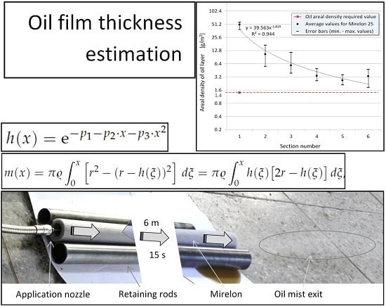
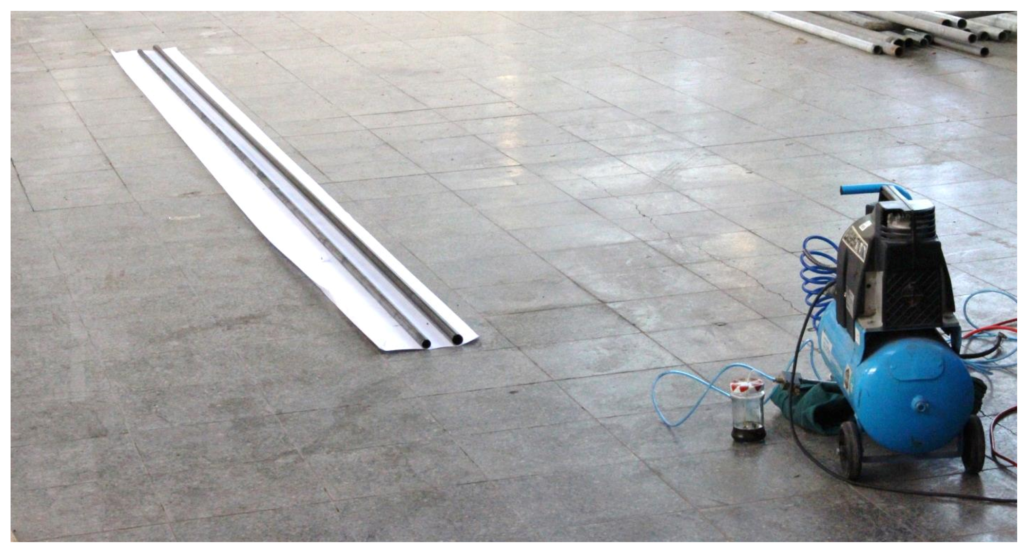
For the experiment of measuring the thickness of the oil layer by applying the oil mist to the interior of the 6 m long thin tubes, the following components were used: oil “Anticorid DFT 2001”; oil mist “SMC LMV210-35”; “Apollo 50” compressor (air receiver 50 L, output power 1.5 kW, supplied air volume 158 L/min) with pressure regulator; calibrated weight “A&D” TSQ 128/95-133 model, d: 0.01 g, e: 0.02 g, carrying capacity: 200 g; accessories for working with compressed air; length gauge; and cutting knife. The overall view of the application environment in the state of preparation before application and measurement is shown in Figure 1. A pair of steel tubes served as a solid support for Mirelon application pipes that are soft and flexible.
Chemical characterization of the oil applied in experimental measurements “Anticorrid DFT 2001”, is specified in the product Safety Data Sheet, according to EU Directive no. 1907/2006, Article 31, Act No. 163/2001 and Decree 515/2001 as a mixture of deeply refined petroleum oils, volatile hydrocarbons and corrosive additives. The oil also contains the following hazardous substances:
- hydrocarbon dearomatized solvent, denoted: Xn, R465, 66 with the concentration of: 50–99%;
- Na-sulfonate, denoted: R53 with the concentration of: 1.2–2.4%;
- solvent naphtha labeled: Xn, Xi, N, R10, 37, 51/53, 65, 66, 67 with the concentration of: 0.1–1%.
The oil parameters according to the Product Card and used in the experimental verification are as follows:
- density: 830 kg/m, at the temperature of 25 C, in compliance with DIN 51 757 standard;
- kinematic viscosity: 4.6 mm/s, at the temperature of 20 C, in compliance with DIN 51 562 standard;
- vapor pressure: 1 mbar, at the temperature of 20 C;
- solubility in water, or miscibility with water: not miscible.
In course of the experimental measurement itself, the following conditions were measured or estimated:
- date of measurement: 30. 12. 2016;
- temperature in the experimental laboratory: 10 C ( C);
- working pressure in the compressor air receiver at the start of oil dispersion application: 8 bar;
- working pressure in the application pistol during the blowing of the oil dispersion: 6 bar;
- the estimated flow rate of the air mix and the dispersed oil fraction in free space: 3 m/s;
- cutting precision of one-meter sections with a length of mm.
Figure 2 shows the course of application of the oil layer onto the inner surface of the tubes. The application lasted 15 s and Fuchs “Anticorid DFT 2001” oil was applied to 6-m long Mirelone tubes. Following the application of the oil through the dispersion oil fraction, the Mirelone tube was divided into one-meter sections, each weighed on the certified scale, Figure 3. First, only a Mirelone tube marked as plain was weighed. Then, the weighing was repeated, this time recording the weight of the tube with oil. The resulting net oil film weight was calculated by simple subtraction.
Figure 4 shows a schematically illustrated pneumatic diagram of device alignment in experimental measurement. Manometer 1 is coupled with the pressure regulator and indicates the pressure set thereon when the latter is active. The manually operated hand valve is a hose of 10 mm in width and 5 m in length.
Measurement scenario for one sample (1-m long tube) was as follows:
- The pressure regulator was set at 8 bar.
- The compressor, which pressurized the air at a pressure of 8 bar into a 50 L vessel, was switched on.
- Six pieces of dry, one meter long application pipes were weighed. Their dry weights were recorded in the metering protocol for later processing.
- One meter long dry pipes were connected in five places to a total length of six meters. The entire dry pipe was placed on the measuring point, and it was important to ensure the pipe’s straightness and pipe tightness at the points of connection.
- The application nozzle was directed at free space and the manual valve was activated for about 3–5 s due to the oil intake into the lubrication feed pipe and also for the tubes to be filled with oil themselves.
- The oil dispersion application nozzle was placed immediately in front of the coated tube. The identical location of the imaginary axis of the nozzle and the axis of the tube was very important. For this reason, the fixture item made on a 3D printer were used for each tube’s inside diameter.
- The manual valve and the timer were activated together.
- After 15 s, the manual valve was deactivated and the oil dispersion stopped flowing into the tube.
- The wet tube (coated with an oil film) was cut into one meter long sections and they were weighed on the precision scale.
- The measured values were recorded in the measurement protocol for further processing.
3. Results of Experimental Measurement
The measured values were processed in the tables, with calculated values of the oil film thickness in each one meter section as a radially uniformly applied layer on the inner surface of the pipe (the thickness of the layer changes in the longitudinal direction) across the entire one-meter section. After processing the measured values, the average area densities of the oil film in the individual measurements for 15, 25 and 35 mm tubes were summarized in Table 1, Table 2 and Table 3. We assume that dividing the measured tubes into one meter long sections is sufficient for a relevant assessment of the presence of the oil film layer on their inner surface. The reason for such division was the practicality of handling the measured sections, ensuring that the accumulated oil does not flow out at the bottom of the pipe section after application. This problem occurred especially in the first and second one-meter sections, which were not of key importance, since, in these sections, the thickness of the oil film layer at each of the considered diameters was sufficient. In addition, the measurement of lower weights that were very close to the dry tube was, in terms of general measurement rules and possibilities to eliminate the resulting uncertainty, more critical. The most critical and most interesting for our purpose were Section 5 and Section 6, with less oil film.
The standard deviation of the weight of one meter of dry Mirelon with a 15 mm inner diameter is 0.082 g, the standard deviation for 25 mm is 0.18 g, and the standard deviation for 35 mm is 0.63 g.
If steel pipes were to be used, it would have been very difficult to measure the oil layer inside the steel pipe as the certified scales with the required carrying capacity are not sufficiently precise and sensitive. The ratio between the weight of the pipe and the weight of the oil film is far more favorable for weighing a material such as “Mirelon”. For example, the dry weight of a 1 m long Mirelon tube with a 25 mm width and a wall thickness of 5 mm weighs approximately 11.5 g, the weight of a steel tube (EN 10 210-2 standard) of 25.3 mm diameter and a wall thickness of 0.8 mm (thinner is not normally produced) weighs approximately 515 g. The dry tube was weighed first, followed by weighing when wet. In percentage points, the differences thus obtained, i.e., between the dry and the wet tube, would have been too small. The measurement of the oil film itself would not have been possible.
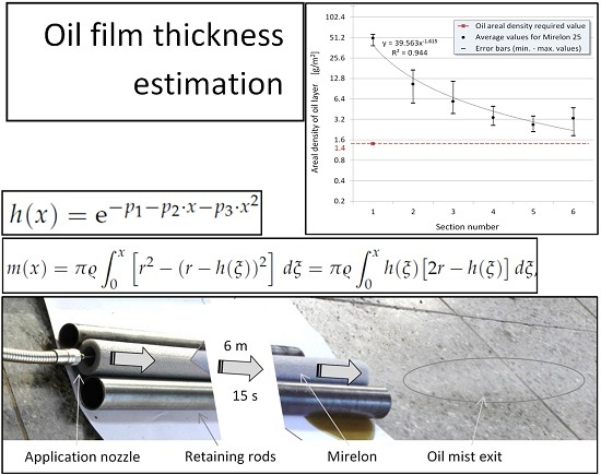
Figure 5 shows graphically represented Table 1, Table 2 and Table 3. Measured average values of the surface density of the oil layer of 15, 25, and 35 mm tubes represent dots of the respective color. The same color depicts the corresponding trendline with the assigned two-parameter power expression and reliability R. The closer the reliability R to 1, the better the trendline/measured data superimposition. All reliability values R are greater than 0.9, which supports the reliability of the transfer of average values measured during the experiment onto the trendline. The 15 mm pipe shows lesser reliability R = 0.9076. This can be explained by the likely leakage of excess oil from a pipe of 15 mm in diameter due to the smallest inner surface where the oil layer is trapped. On this smallest area, a freely flowing oil layer was produced in the first one-meter section, which was slightly tilted from the application of the dispersion oil fraction to the scale, and leaked a smaller amount of oil. However, in spite of this measurement imperfection, it was found that the measurement was not significantly affected, since the important oil layer thicknesses were found in the 1-m sections, number 3–6. In the first two 1-m sections, the oil film layer was always sufficient at any pipe diameter and the given parameters.
Furthermore, Figure 5 shows that only the trendline for a 25 mm tube does not touch the oil-saturation limit value that corresponds to the manufacturer’s prescribed value of 1.4 g/m. However, consideration should be given to the possible scattering of the individual measured values, and therefore a perfect oil layer inside the pipe, which complies with the manufacturer’s instructions, is not guaranteed. Trendlines for a slim tube of 15 mm and a thick tube of 35 mm for the limit of 1.4 g/m are intersected closely at the intersection of the fourth and fifth measuring points. It should be noted that the vertical axis in Figure 5 has a logarithmic scale to better plot the graph with the measured data.
4. Oil Film Layer Thickness Estimation
In this section, we describe the processing of the data obtained by simulation and measured weight data of the anticorrosive liquid ANTICORIT DFV 2001, hereinafter referred to as “oil”, on the individual one-meter pipe sections, with a total considered length of 6 m. Our goal is to obtain a lower (pessimistic) estimate of the thickness of the oil film layer to ensure compliance with the FLV-F3 standard derived from our own FUCHS laboratory method, i.e., the areal density of the oil film g/m. The areal density in the given position will be equal to , where h is the layer thickness, and kg/m is the oil volume density, in compliance with the DIN 51 757 standard. The critical value of corresponds to the critical layer thickness of m m.
While we expect a cylindrical symmetric thickness of the oil layer, let us suppose that the oil is angular, uniformly distributed in the pipe, so the oil film thickness depends only on the distance x from the pipe’s end. Let it be denoted , , where l is the length of a pipe. Then, the total oil mass from the pipe’s beginning at to the point x is defined by the relation
where is the pipe’s inner radius. The oil mass at the i-th pipe section between the points and , , 2, ..., n will then be equal to
For example, the oil mass in the 2nd section of a 1-m length, established in an experimental measurement, will be equal to .
Given the small number of data, we have decided to determine the appropriate, not very complex, dependence of so that the theoretical mass values correspond quite well to the measured values, but do not exceed them, especially in sections with a lower assumed areal density of the oil layer, i.e., further from the injection point.
Due to the big relative differences between measured values for different sections, measured values logarithms are shown in Figure 5. Logarithms of measured values can be approximated also by linear functions with similar precision as is the precision of the shown trendlines. Therefore, we decided to use exponential functions first. Another reason for a choice of exponential functions is that the function in (1) can be calculated analytically for such functions.
If the oil film thickness has an exponential form
then using few commands of an open-source Computer Algebra System (CAS) wxMaxima (version 16.04.2, General Public License) [17]:
assume(x>0); h:h0*exp(-a*x); h:h*exp(-a*x);
M:%pi*rho*integrate((r^2-(r-subst(t,x,h))^2),t,0,x); tex(%);one arrives at a formula
The oil masses within individual one-meter sections are:
where is the oil density.
It is evident that “theoretical” masses (5) decrease almost exponentially, similarly to the oil film thickness .
Experimentally measured values—oil film mean masses in individual one-meter long sections , 2, ..., 6—were compared to theoretical values , , 2, ..., 6 according to Equations (2) and (5), obtained from integrals (1). Figure 6 shows logarithms of the measured data with an asterisk marking for six segments of the one meter length, and the logarithms of theoretical masses (5) calculated for a case of an exponential dependence of the thickness (3) on the distance x. The respective parameters and a are given in the legends. The bottom “theoretical” circles serve as the lower “exponential” bounds (with one exception of one measurement for 25 mm pipe, see Figure 6b) for the oil mass distribution.
Furthermore, we were comparing various dependency types, for example those given in [16] and we finally decided to use a three-parametric dependency in the exponential form:
adding one new parameter to the right side in the Equation (3).
We calculated the integrals (1) using the Simpson’s rule of numerical integration [18,19]. The calculation made use of another open-source program Octave (GNU Octave ver. 4.2.1, General Public License, Free Software Foundation) [20]. For our purpose, Octave is of equal usability as a commercial program MATLAB (The MathWorks, Inc., Natick, Massachusetts, USA) [21]. Functions and scripts used in one of these programs can be used in the other program practically change-free. Therefore, we recommend Octave to potential programmers. Initial parameter estimates were obtained using the Nelder–Mead Minimization Method [22,23,24]. The author of the function nelder_mead_min is Etienne Grossmann, inspired by the book [19].
Figure 7, Figure 8 and Figure 9 compare the results of experimental data approximation using functions of the form (6) via minimization based on four different criteria. We minimized the functions of two vector deviations in various norms:
- ;
- ;
- ;
- .
Figure 7 shows the minimization results for 15 mm pipes. Criteria 2 and 4 lead to excessively large underestimation of the measured masses, the results based on criterion 3 are applicable, but the theoretical value of the mass is higher in the third section. Therefore, we determined the appropriate parameters manually—the result is marked by number 5.
Looking at the pictures in Figure 8, we can state that, out of the four possibilities mentioned, only the parameters obtained by application of the 4th method meet the condition of the lower estimate mentioned above—the theoretical oil mass is greater than the measured mass only in the 2nd section. We can expect that the minimum theoretical thickness, corresponding with the dependency (6) for parameter values given in the last line of the Table 4, provides the lower estimate of the actual minimum thickness of the oil film. The respective optimum parameters for different criteria application to measure individual deviations from average mass values of oil films in the 25-mm pipes are stated in the Table 4.
Figure 9 shows the minimization results for 35 mm pipes. Only the criterion number 3 yields appropriate results, with theoretical mass values higher in the 2nd and the 3rd section, respectively. This is why we determined the appropriate parameters manually also in this case—the result is marked by number 5.
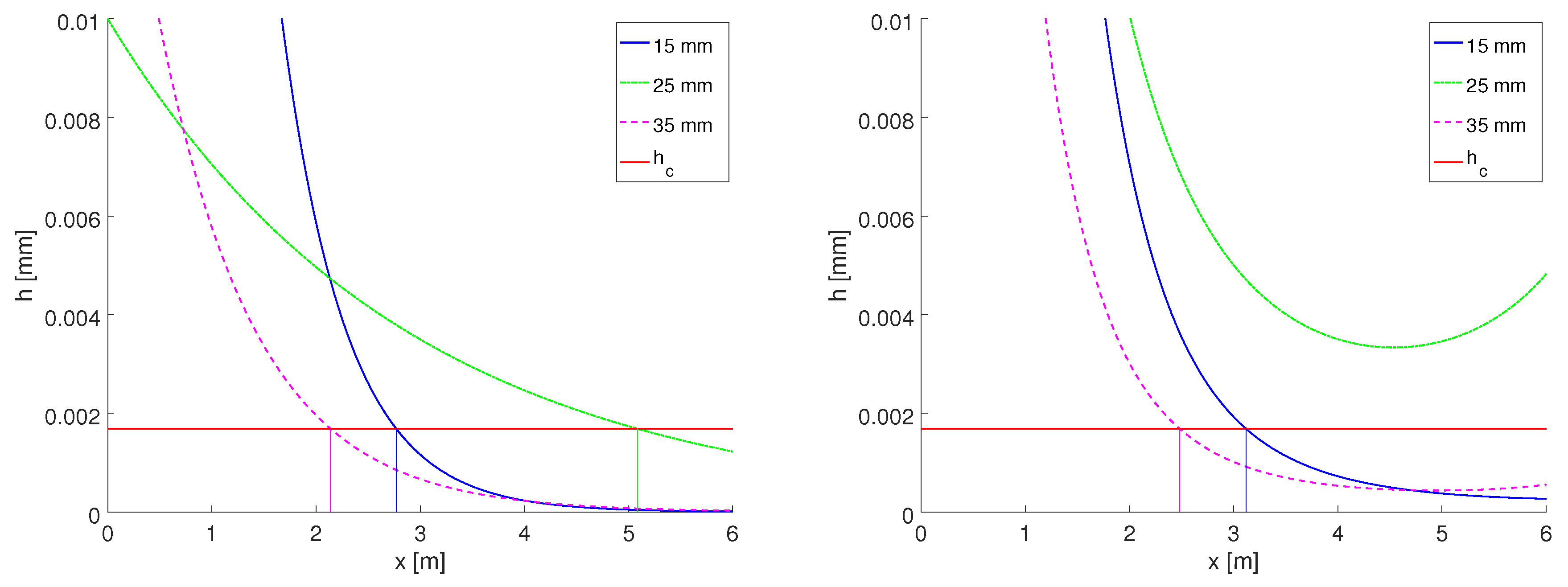
Figure 10 (left) shows oil film thickness dependencies on the distance x—the position of the point from the place of the oil mist injection—for optimal parameter values for the exponential model (3). In pipes of 15 mm in diameter, the “sufficient film thickness” stretches only half way through. The suitable layer in the 25 mm diameter pipes is along the whole length. The tubes of the largest diameter 35 mm have a much larger thickness at their start (we cannot see the corresponding parts of the curves because we chose a common vertical scale for better comparison); however, only about 2 m have the sufficient oil film thickness.
Figure 10 (right) shows the situation for the “exponential” model (6). It seems that we can expect that, at the given oil mist injection mode, the thickness of the film of a 25 mm pipe will be everywhere above the critical value of m. In the case of a 15 mm pipe, we can expect that up to the intersection point 3.11 m, the oil film thickness will be greater than critical; therefore, upon the oil mist injection from both sides, a sufficient thick film should form alongside the entire pipe. In the case of 35 mm pipes, the “critical” value is m, i.e., the injection mode needs adjusting.
5. Discussion
One of the main contributions of the article is the derivation of relations for the practical estimation of the thickness of the oil layer, which is applied by means of the dispersed oil fraction under the given conditions.
The flow of the dispersed oil fraction inside the lean tube is influenced by a number of variables and factors entering this process. In addition, the measurement errors, the nozzle angle adjustment and the depth of its insertion into the pipe, as well as the design and condition of the inner surface of the pipe itself, have a considerable impact on the results of measuring the distance of the impact of oil microparticles. For these reasons, the basic conditions for approximation were defined so as to guarantee a pessimistic (i.e., in graphical representation the lower) estimate of the oil film thickness.
The results also show the large influence of tube diameter on the distance of the microparticles of the application liquid. Three tube diameters were investigated, with two methods applied, and, in one case, given the parameters, the method did not provide sufficient results suitable for application. However, after adjusting, the designed parameters of the applied layer were attained, such as: flow rates, application time, fraction density, temperature, etc.—this is a prerequisite for fulfilling the desired parameters of the coated layer.
As can be seen from the previous graphical representation, under the same application conditions, the dispersed oil fraction in different diameter pipes behaves differently. In the test pipe of middle diameter, the oil microparticles fell the furthest and in greatest abundance, to form a coherent oil film of sufficient thickness. For other pipe diameters, it is recommended to apply a dispersion oil fraction from both sides of the lean pipe, to obtain a sufficiently thick oil film as prescribed by the oil manufacturer. In the case of the largest-diameter pipe, it is advisable to extend the time span so that a sufficient quantity of oil microparticles travels a sufficient distance up to the mid-length of the pipe. In each of these cases, when applying a dispersed oil fraction, it is recommended to rotate the coated pipe around its longitudinal axis to distribute the oil film uniformly in the radial direction. This rotation, as well as application of the dispersion oil fraction from both sides of the pipe, is not a problem in practical technical applications.
From the viewpoint of monitoring the coating process, it is a good choice for this challenging process to use an experimental system designed and developed for multi-parametric simulated monitoring of technical systems [25], but it is still necessary to adhere to commonly used [26] standards. It is appropriate to optimize the proposed process. In general, computer-aided optimization technologies are recommended [27].
6. Conclusions
The result of our research is a realistic method for estimating the distance of particle impact of the dispersed oil fraction for different inner diameters of slim tubes. The relationships and methods listed above are sufficient to provide a relatively accurate lower estimate of the thickness of the oil layer under the operating conditions. For steel pipes with a standard length of 6 m and an internal diameter in the range of 15 to 35 mm, the steel tube is anticorrosively modified from the device by applying the dispersion oil fraction to the device under normal operating conditions such as operating temperature 15 to 25 C, compressed air pressure in the range from 5 to 8 bar. The condition is to keep the 20 s application time, continuous pipe rotation during and/or after the application and the application from both sides of the oven will be necessary. As mentioned above (see also Figure 10 (right)), we can expect that, at the given oil mist injection mode, the thickness of the film of a 25 mm pipe will be everywhere above the critical value of m. In the case of a 15 mm pipe, a lower bound exponential line intersects the critical value at the point m, so we may expect that at least one half of the pipe will be covered by the oil film with sufficient thickness. In the case of 35 mm pipes, the “critical” value is m, which is less than one half of the pipe’s length, i.e., the injection mode needs adjusting.
In case of time optimization and avoidance of duplex application, for example in large-scale production, it is possible to analyze, according to the analyzed methodology, the thickness of the applied oil layer. For other internal diameters and pipe lengths, we recommend experimentally verifying the thickness of the oil layer.
Acknowledgments
This research work was supported by projects: APVV-15-0149 “Research of new measuring methods of machine condition”, VEGA 1/0437/17 “Research and development of rotary module with an unlimited degree rotation” and APVV-15-0202 “Development equipment for efficient compression and storage of hydrogen using new metal hydride alloys”. We thank unknown reviewers for valuable recommendations of text improvement.
Author Contributions
Jozef Svetlík suggested the concept of coating the inner surface of slim tubes with of a dispersed oil fraction; Ján Král’ and Jozef Svetlík designed and performed experimental measurements in the laboratory; Ján Buša analyzed the data and suggested a calculation model for estimating the thickness of the oil layer; Tomáš Brestovič performed a numerical coating simulation; Jozef Dobránsky contributed materials and analysis tools; Jozef Svetlík and Ján Buša wrote the paper.
Conflicts of Interest
The authors declare no conflict of interest. The founding sponsors had no role in the design of the study; in the collection, analyses, or interpretation of data; in the writing of the manuscript, and in the decision to publish the results.
References
- Fuchs Oil Corporation. Available online: https://www.fuchs.com/pl/en/company/about-fuchs/company-portrait/ (accessed on 25 August 2017).
- Chigondo, M.; Chigondo, F. Recent Natural Corrosion Inhibitors for Mild Steel: An Overview. J. Chem. 2016. [Google Scholar] [CrossRef]
- Lgaz, H.; Belkhaouda, M.; Larouj, M.; Salghi, R.; Jodeh, S.; Warad, I.; Oudda, H.; Chetouani, A. Corrosion Protection of Carbon Steel in Acidic Solution by Using Ylang-Ylang Oil as Green Inhibitor. Moroc. J. Chem. 2016, 4, 101–111. [Google Scholar]
- Kashif, M.; Ahmad, S. Polyorthotoluidine dispersed castor oil polyurethane anticorrosive nanocomposite coatings. RSC Adv. 2014, 4, 20984–20999. [Google Scholar] [CrossRef]
- Pourhashem, S.; Vaezi, M.R.; Rashidi, A.; Bagherzadeh, M.R. Exploring corrosion protection properties of solvent based epoxy-graphene oxide nanocomposite coatings on mild steel. Corros. Sci. 2017, 115, 78–92. [Google Scholar] [CrossRef]
- Zhang, B.; Feng, H.T.; Lin, F.; Wang, Y.B.; Wang, L.P.; Dong, Y.P.; Li, W. Superhydrophobic surface fabricated on iron substrate by black chromium electrodeposition and its corrosion resistance property. Appl. Surf. Sci. 2016, 378, 388–396. [Google Scholar] [CrossRef]
- Zavareh, M.A.; Sarhan, A.A.D.M.; Zavareh, P.A.; Razak, B.B.A.; Basirun, W.; Ismail, M.B.C. Development and protection evaluation of two new, advanced ceramic composite thermal spray coatings, Al2O3-40TiO(2) and Cr3C2-20NiCr on carbon steel petroleum oil piping. Ceram. Int. 2016, 42, 5203–5210. [Google Scholar] [CrossRef]
- Mallozzi, M.; Kehr, J.A. Nano-Technology for Improved Dual Layer Performance. In Proceedings of the ASME International Pipeline Conference, Calgary, AB, Canada, 29 September–3 October 2008; AMER SOC Mechanical Engineers: Calgary, AB, Canada, 2008. [Google Scholar]
- Shameli, E. Thickness evaluation of insulated pipelines and pressure vessels using pulsed eddy current technology. In Proceedings of the ASME 2012 International Mechanical Engineering Congress and Exposition, Houston, TX, USA, 9–15 November 2012. [Google Scholar]
- Ma, T.; Feng, L.; Wang, H.; Liu, H.; Yao, M. A numerical study of spray/wall impingement based on droplet impact phenomenon. Int. J. Heat Mass Transf. 2017, 112, 401–412. [Google Scholar] [CrossRef]
- Tang, C.; Qin, M.; Weng, X.; Zhang, X.; Zhang, P.; Li, J.; Huang, Z. Dynamics of droplet impact on solid surface with different roughness. Int. J. Multiph. Flow 2017, 96, 56–69. [Google Scholar] [CrossRef]
- Mahsa, E.; Ortega, A. An experimental technique for accelerating a single liquid droplet to high impact velocities against a solid target surface using a propellant gas. Exp. Therm. Fluid Sci. 2017, 81, 202–208. [Google Scholar]
- Gulraiz, A.; Seller, M.; Chu Lee, Y.; Jermy, M.; Taylor, M. Modeling the spreading and sliding of power-law droplets. Colloids Surf. A Physicochem. Eng. Asp. 2013, 432, 2–7. [Google Scholar]
- Legendre, D.; Maglio, M. Numerical simulation of spreading drops. Colloids Surf. A Physicochem. Eng. Asp. 2013, 432, 29–37. [Google Scholar] [CrossRef] [Green Version]
- Svetlík, J.; Král’, J.; Brestovič, T.; Pituk, M. Device for applying a thin layer of oil onto the inner surface of steel pipes. Manuf. Technol. 2017, 17, 257–260. [Google Scholar]
- Svetlík, J.; Buša, J.; Brestovič, T.; Pituk, M.; Pešková, A.; Dudová, P. Research into oil film coating of a steel pipe interior by oil mist blowing. Metalurgija 2018, 57. [Google Scholar]
- wxMaxima. Available online: http://andrejv.github.io/wxmaxima/index.html (accessed on 25 August 2017).
- Kreyszig, E. Simpson’s Rule of Integration. In Advanced Engineering Mathematics; John Wiley & Sons, Inc.: Hoboken, NJ, USA, 2011; pp. 831–832. [Google Scholar]
- Press, W.H.; Teukolsky, S.H.; Vetterling, V.T.; Flannery, B.P. Numerical recipes. In C: The Art of Scientific Computing, 2nd ed.; Cambridge University Press: Cambridge, UK, 1992; p. 994. [Google Scholar]
- GNU Octave. Available online: https://www.gnu.org/software/octave/ (accessed on 25 August 2017).
- MATLAB—MathWorks. Available online: https://www.mathworks.com/products/matlab.html (accessed on 25 August 2017).
- Gill, P.E.; Murray, W.; Wright, M.H. Practical Optimization; Academic Press, Ltd.: Cambridge, MA, USA, 1981; p. 402. ISBN 0-12-283950-1. [Google Scholar]
- Nelder, J.A.; Mead, R. A simplex method for function minimization. Comput. J. 1965, 7, 308–313. [Google Scholar] [CrossRef]
- Spendley, W.; Hext, G.R.; Himsworth, F.R. Sequential application of simplex designs in optimization and evolutionary design. Technometrics 1962, 4, 441–461. [Google Scholar] [CrossRef]
- Murcinkova, Z.; Krenický, T. Implementation of virtual instrumentation for multiparametric technical system monitoring. In Proceedings of the International Multidisciplinary Scientific GeoConference, Albena, Bulgaria, 16–22 June 2013; pp. 139–144. [Google Scholar]
- Pitel’, J.; Tóthová, M.; Židek, K. Technical Measurement and Diagnostics; Technical University of Košice: Košice, Slovakia, 2015; p. 117. [Google Scholar]
- Dobránsky, J.; Baron, P.; Vojnová, E.; Mandul’ák, D. Optimization of the production and logistics processes based on computer simulation tools. Key Eng. Mater. 2016, 669, 532–540. [Google Scholar] [CrossRef]
Figure 1.
Application environment for experimental coating of inner surface of tubes by dispersion oil fraction and equipment.
Figure 1.
Application environment for experimental coating of inner surface of tubes by dispersion oil fraction and equipment.

Figure 2.
Method of application of oil mist during the experiment.

Figure 3.
Weighing of the meter sections after application of the dispersion oil fraction.
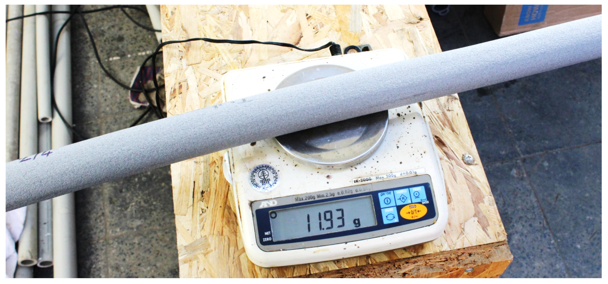
Figure 4.
Pneumatic wiring diagram for experimental measurement of coating of the inner surface of an oil dispersion tube.
Figure 4.
Pneumatic wiring diagram for experimental measurement of coating of the inner surface of an oil dispersion tube.

Figure 5.
Average values of experimental measurements for all pipe diameters, i.e., 15, 25, and 35 mm. Trendlines demonstrate different behaviour of oil microparticles in tubes of different diameters. Flow rate was constant at all measurements.
Figure 5.
Average values of experimental measurements for all pipe diameters, i.e., 15, 25, and 35 mm. Trendlines demonstrate different behaviour of oil microparticles in tubes of different diameters. Flow rate was constant at all measurements.

Figure 6.
Lower and upper exponential bounds (marked by circles) in the logarithmic scale for (a) 15 mm, (b) 25 mm, and (c) 35 mm pipes.
Figure 6.
Lower and upper exponential bounds (marked by circles) in the logarithmic scale for (a) 15 mm, (b) 25 mm, and (c) 35 mm pipes.
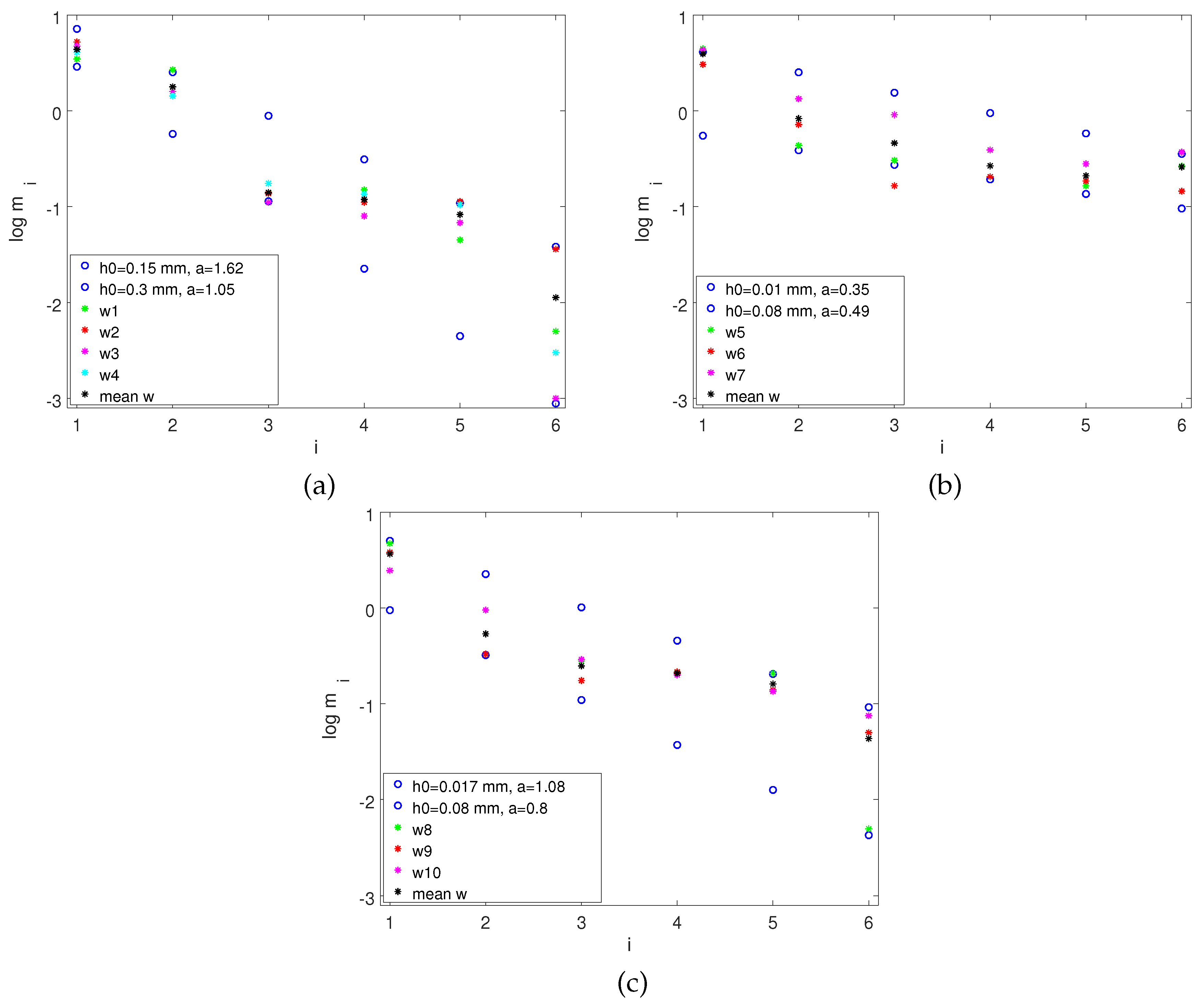
Figure 7.
(a) theoretical values of the logarithms (asterisk * marks measured values) describing average values of 15-mm pipes; (b) deviations of theoretical logarithms of the values of from logarithms of the values obtained experimentally, , ..., 6 for criteria 1–4.
Figure 7.
(a) theoretical values of the logarithms (asterisk * marks measured values) describing average values of 15-mm pipes; (b) deviations of theoretical logarithms of the values of from logarithms of the values obtained experimentally, , ..., 6 for criteria 1–4.

Figure 8.
(a) theoretical values of the logarithms (asterisk * marks measured values) describing average values of 25-mm pipes; (b) deviations of theoretical logarithms of the values of from logarithms of the values obtained experimentally, , ..., 6 for criteria 1–4.
Figure 8.
(a) theoretical values of the logarithms (asterisk * marks measured values) describing average values of 25-mm pipes; (b) deviations of theoretical logarithms of the values of from logarithms of the values obtained experimentally, , ..., 6 for criteria 1–4.
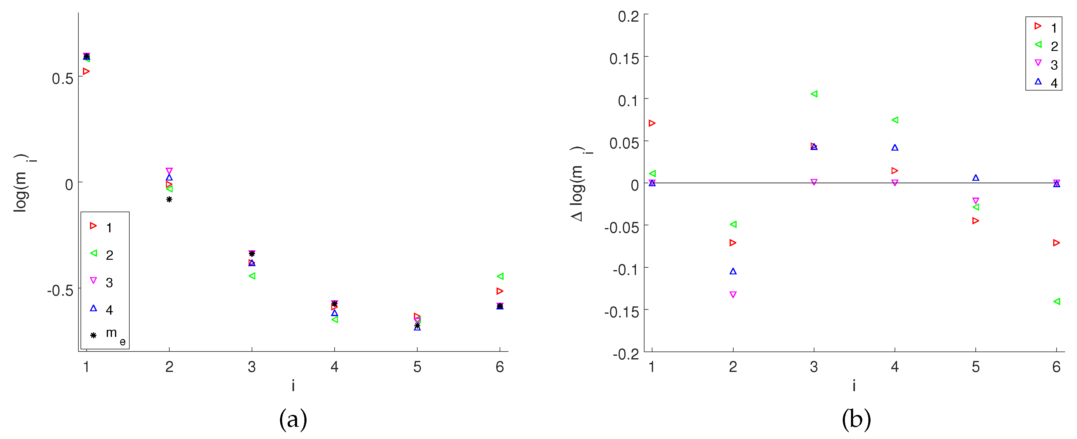
Figure 9.
(a) theoretical values of the logarithms (asterisk * marks measured values) describing average values of 35-mm pipes; (b) deviations of theoretical logarithms of the values of from logarithms of the values obtained experimentally, , ..., 6 for criteria 1–4.
Figure 9.
(a) theoretical values of the logarithms (asterisk * marks measured values) describing average values of 35-mm pipes; (b) deviations of theoretical logarithms of the values of from logarithms of the values obtained experimentally, , ..., 6 for criteria 1–4.
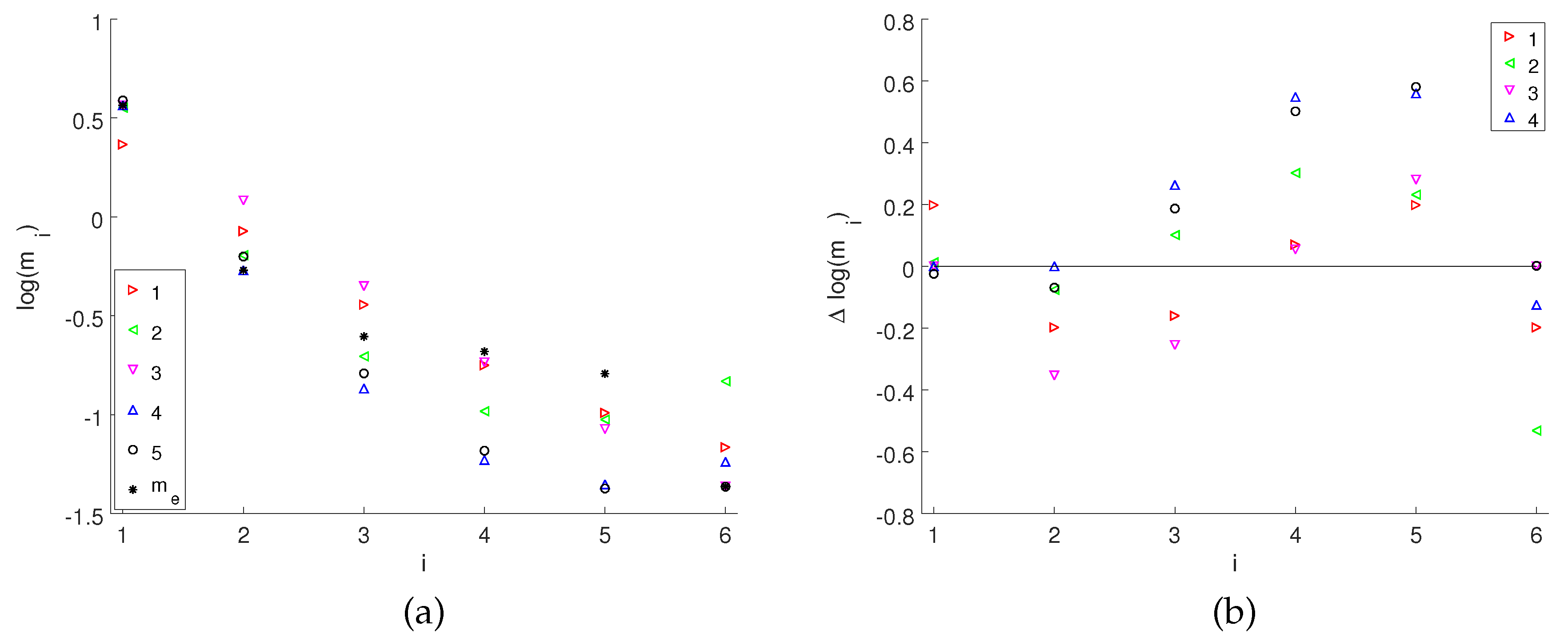
Figure 10.
The course of the thickness of the oil layer in model dependencies for different pipe diameter values—15, 25 and 35 mm (critical value is m).
Figure 10.
The course of the thickness of the oil layer in model dependencies for different pipe diameter values—15, 25 and 35 mm (critical value is m).

Table 1.
Average values of the oil film areal density (in g/m) in a 15-mm slim pipe. The section length is 1 m. The total measured pipe length is 6 m.
Table 1.
Average values of the oil film areal density (in g/m) in a 15-mm slim pipe. The section length is 1 m. The total measured pipe length is 6 m.
| Sector | 1 | 2 | 3 | 4 | 5 | 6 |
|---|---|---|---|---|---|---|
| 1. measurement | 73.74 | 56.97 | 2.97 | 3.18 | 0.95 | 0.10 |
| 2. measurement | 110.94 | 30.22 | 2.91 | 2.36 | 2.39 | 0.76 |
| 3. measurement | 100.35 | 33.78 | 2.36 | 1.70 | 1.44 | 0.02 |
| 4. measurement | 86.68 | 30.22 | 3.71 | 2.86 | 2.23 | 0.06 |
| Average value | 92.93 | 37.80 | 2.99 | 2.53 | 1.76 | 0.24 |
Table 2.
Average values of the oil film areal density (in g/m) in a 25-mm slim pipe. The section length is 1 m. The total measured pipe length is 6 m.
Table 2.
Average values of the oil film areal density (in g/m) in a 25-mm slim pipe. The section length is 1 m. The total measured pipe length is 6 m.
| Sector | 1 | 2 | 3 | 4 | 5 | 6 |
|---|---|---|---|---|---|---|
| 1. measurement | 56.47 | 5.54 | 3.88 | 2.61 | 2.10 | 3.38 |
| 2. measurement | 38.83 | 9.17 | 2.10 | 2.61 | 2.36 | 1.85 |
| 3. measurement | 54.69 | 17.00 | 11.59 | 4.97 | 3.57 | 4.71 |
| Average value | 49.99 | 10.57 | 5.86 | 3.40 | 2.68 | 3.31 |
Table 3.
Average values of the oil film areal density (in g/m) in a 35-mm slim pipe. The section length is 1 m. The total measured pipe length is 6 m.
Table 3.
Average values of the oil film areal density (in g/m) in a 35-mm slim pipe. The section length is 1 m. The total measured pipe length is 6 m.
| Sector | 1 | 2 | 3 | 4 | 5 | 6 |
|---|---|---|---|---|---|---|
| 1. measurement | 42.84 | 3.00 | 2.55 | 1.91 | 1.89 | 0.05 |
| 2. measurement | 34.65 | 3.00 | 1.59 | 1.96 | 1.27 | 0.45 |
| 3. measurement | 22.37 | 8.64 | 2.64 | 1.82 | 1.23 | 0.68 |
| Average value | 33.29 | 4.88 | 2.26 | 1.89 | 1.46 | 0.39 |
Table 4.
Optimum dependency coefficients (6) for criteria 1–4 for average values of 25 mm pipes.
| Method | |||
|---|---|---|---|
| 1 | 9.238 | 1.559 | |
| 2 | 9.010 | 1.822 | |
| 3 | 9.071 | 1.561 | |
| 4 | 9.040 | 1.652 |
© 2017 by the authors. Licensee MDPI, Basel, Switzerland. This article is an open access article distributed under the terms and conditions of the Creative Commons Attribution (CC BY) license (http://creativecommons.org/licenses/by/4.0/).
Share and Cite
MDPI and ACS Style
Svetlík, J.; Buša, J.; Brestovič, T.; Dobránsky, J.; Kráľ, J. Film Thickness Estimation for the Oil Applied to the Inner Surface of Slim Tubes. Appl. Sci. 2017, 7, 977. https://doi.org/10.3390/app7100977
AMA Style
Svetlík J, Buša J, Brestovič T, Dobránsky J, Kráľ J. Film Thickness Estimation for the Oil Applied to the Inner Surface of Slim Tubes. Applied Sciences. 2017; 7(10):977. https://doi.org/10.3390/app7100977
Chicago/Turabian StyleSvetlík, Jozef, Ján Buša, Tomáš Brestovič, Jozef Dobránsky, and Ján Kráľ. 2017. "Film Thickness Estimation for the Oil Applied to the Inner Surface of Slim Tubes" Applied Sciences 7, no. 10: 977. https://doi.org/10.3390/app7100977
Note that from the first issue of 2016, this journal uses article numbers instead of page numbers. See further details here.