A Software Reliability Model with a Weibull Fault Detection Rate Function Subject to Operating Environments

1
Department of Computer Science and Statistics, Chosun University, 309 Pilmun-daero Dong-gu, Gwangju 61452, Korea
2
Department of Industrial and Systems Engineering, Rutgers University, 96 Frelinghuysen Road, Piscataway, NJ 08855-8018, USA
*
Author to whom correspondence should be addressed.
Appl. Sci. 2017, 7(10), 983; https://doi.org/10.3390/app7100983
Submission received: 21 August 2017
/
Revised: 20 September 2017
/
Accepted: 22 September 2017
/
Published: 25 September 2017
Abstract
:Featured Application
This study introduces a new software reliability model with the Weibull fault detection rate function that takes into account the uncertainty of operating environments.
Abstract
When software systems are introduced, these systems are used in field environments that are the same as or close to those used in the development-testing environments; however, they may also be used in many different locations that may differ from the environment in which they were developed and tested. As such, it is difficult to improve software reliability for a variety of reasons, such as a given environment, or a bug location in code. In this paper, we propose a new software reliability model that takes into account the uncertainty of operating environments. The explicit mean value function solution for the proposed model is presented. Examples are presented to illustrate the goodness of fit of the proposed model and several existing non-homogeneous Poisson process (NHPP) models and confidence intervals of all models based on two sets of failure data collected from software applications. The results show that the proposed model fits the data more closely than other existing NHPP models to a significant extent.
1. Introduction
Software systems have become an essential part of our lives. These systems are very important because they are able to ensure the provision of high-quality services to customers due to their reliability and stability. However, software development is a difficult and complex process. Therefore, the main focus of software companies is on improving the reliability and stability of a software system. This has prompted research in software reliability engineering and many software reliability growth models (SRGM) have been proposed over the past decades. Many existing non-homogeneous Poisson process (NHPP) software reliability models have been developed through the fault intensity rate function and the mean value functions within a controlled testing environment to estimate reliability metrics such as the number of residual faults, failure rate, and reliability of software. Generally, the reliability increases more quickly and later the improvement slows down. Software reliability models are used to estimate and predict the reliability, number of remaining faults, failure intensity, total software development cost, and so forth, of software. Various software reliability models and application studies have been developed to date. Discovering the confidence intervals of software reliability is done in the field of software reliability because it can enhance the decision of software releases and control the related expenditures for software testing [1]. First, Yamada and Osaki [2] considered that the maximum likelihood estimates concerning the confidence interval of the mean value function can be estimated. Yin and Trivedi [3] present the confidence bounds for the model parameters via the Bayesian approach. Huang [4] also present a graph to illustrate the confidence interval of the mean value function. Gonzalez et al. [5] presented a general methodology that applied to a power distribution test system considering the effect of weather conditions and aging of components in the system reliability indexes for the analysis of repairable systems using non-homogeneous Poisson process, including several conditions in the system at the same time. Nagaraju and Fiondella [6] presented an adaptive expectation-maximization algorithm for non-homogeneous Poisson process software reliability growth models, and illustrated the steps of this adaptive approach through a detailed example, which demonstrates improved flexibility over the standard expectation-maximization (EM) algorithm. Srivastava and Mondal [7] proposed a predictive maintenance model for an N-component repairable system by integrating non-homogeneous Poisson process (NHPP) models and system availability concept, such that the use of costly predictive maintenance technology is minimized. Kim et al. [8] described application of the software reliability model of the target system to increase the software reliability, and presented some analytical methods as well as the prediction and estimation results.
Chatterjee and Singh [9] proposed a software reliability model based on NHPP that incorporates a logistic-exponential testing coverage function with imperfect debugging. In addition, Chatterjee and Shukla [10] developed a software reliability model that considers different types of faults incorporating both imperfect debugging and a change point. Yamada et al. [11] developed a software-reliability growth model incorporating the amount of test effort expended during the software testing phase. Joh et al. [12] proposed a new Weibull distribution based on vulnerability discovery model. Sagar et al. [13] presented best software reliability growth model with including feature of both Weibull distribution and inflection S-shaped SRGM to estimate the defects of software system, and provide help to researchers and software industries to develop highly reliable software products.
Generally, existing models are applied to software testing data and then used to make predictions on the software failures and reliability in the field. Here, the important point is that the test environment and operational environment are different from each other. Once software systems are introduced, the software systems used in the field environments are the same as or close to those used in the development-testing environment; however, the systems may be used in many different locations. Several researchers started applying the factor of operational environments. A few researchers, Yang and Xie, Huang et al., and Zhang et al. [14,15,16], proposed a method of predicting the fault detection rate to reflect changes in operating environments, and used methodology that modifies the software reliability model in the operating environments by introducing a calibration factor. Teng and Pham [17] discussed a generalized model that captures the uncertainty of the environment and its effects upon the software failure rate. Pham [18,19] and Chang et al. [20] developed a software reliability model incorporating the uncertainty of the system fault detection rate per unit of time subject to the operating environment. Honda et al. [21] proposed a generalized software reliability model (GSRM) based on a stochastic process and simulated developments that include uncertainties and dynamics. Pham [22] recently presented a new generalized software reliability model subject to the uncertainty of operating environments. And also, Song et al. [23] presented a new model with consideration of a three-parameter fault detection rate in the software development process, and relate it to the error detection rate function with consideration of the uncertainty of operating environments.
In this paper, we discuss a new model with consideration for the Weibull function in the software development process and relate it to the error detection rate function with consideration of the uncertainty of operating environments. We examine the goodness of fit of the fault detection rate software reliability model and other existing NHPP models based on several sets of software testing data. The explicit solution of the mean value function for the new model is derived in Section 2. Criteria for model comparisons and confidence interval for selection of the best model are discussed in Section 3. Model analysis and results are discussed in Section 4. Section 5 presents the conclusions and remarks.
2. A New Software Reliability Model
In this section, we propose a new NHPP software reliability model. First, we describe the NHPP software reliability model and present a solution of the new mean value function considering the new fault detection rate function against the generalized NHPP software reliability model, incorporating the uncertainty of fault detection rate per unit of time in the operating environments.
2.1. Non-Homogeneous Poisson Process Model
The software fault detection process has been widely formulated by using a counting process. A counting process, {}, is said to be a non-homogeneous Poisson process with intensity function if follows a Poisson distribution with the mean value function , namely,
The mean value function , which is the expected number of faults detected at time , can be expressed as
where represents the failure intensity.
A general framework for NHPP-based SRGM has been proposed by Pham et al. [24]. They have modeled using the differential equation
Solving Equation (1) makes it possible to obtain different values of using different values for and , which reflects various assumptions of the software testing process.
2.2. Weibull Fault Detection Rate Function Model
A generalized NHPP model incorporating the uncertainty of operating environments can be formulated as follows [19]:
where is a random variable that represents the uncertainty of the system fault detection rate in the operating environments with a probability density function , is the expected number of faults that exists in the software before testing, is the fault detection rate function, which also represents the average failure rate of a fault, and m(t) is the expected number of errors detected by time or the mean value function. We propose an NHPP software reliability model, including the uncertainty of the operating environment using Equation (2) and the following assumptions [19,23]:
- (a)
- The occurrence of software failures follows an NHPP.
- (b)
- Software can fail during execution, caused by faults in the software.
- (c)
- The software-failure detection rate at any time is proportional to the number of remaining faults in the software at that time.
- (d)
- When a software failure occurs, a debugging effort removes the faults immediately.
- (e)
- For each debugging effort, regardless of whether the faults are successfully removed, some new faults may be introduced into the software system.
- (f)
- The environment affects the unit failure detection rate, , by multiplying by a factor .
The solution for the mean value function m(t), where the initial condition m(0) = 0, is given by [19]:
Pham [22] recently developed a generalized software reliability model incorporating the uncertainty of fault detection rate per unit of time in the operating environments where the random variable η has a generalized probability density function g with two parameters, and , and the mean value function from Equation (3) is given by:
where b(t) is the fault detection rate per fault per unit of time.
The Weibull distribution is one of the most commonly used distributions for modeling irregular data, is very easy to interpret and very useful. The Weibull distribution is a distribution that can be used instead of a normal distribution for data with a bias, and used lifetime distributions in reliability engineering. Weibull distribution has been applied in the area of reliability quality control duration, and failure time modelling. This distribution can be widely and effectively used in reliability applications because it has wide variety of shapes in its density and failure rate functions, making it useful for fitting many types of data. In the modelling software development was often described by Weibull-type curves. The discrete Weibull distribution can describe flexibility stochastic behavior of the failure occurrence times. The Weibull-based method is significantly better than the Laplacian-based rate prediction. Both logistic and Weibull distributions will result in a cumulative distribution function with an S-shaped for the lifetime software product [25,26].
In this paper, we consider a Weibull fault detection rate function to be as follows:
where and are known as the scale and shape parameters, respectively. A Weibull fault detection rate function is decreasing for , increasing for , and constant when . We obtain a new NHPP software reliability model subject to the uncertainty of the environments, m(t), that can be used to determine the expected number of software failures detected by time by substituting the function b(t) above into Equation (4):
3. Model Comparisons
In this section, we present a set of comparison criteria for best model selection, quantitatively compare the models using these comparison criteria, and obtain the confidence intervals of the NHPP software reliability model.
3.1. Criteria for Model Comparisons
Once the analytical expression for the mean value function is derived, the model parameters to be estimated in the mean value function can then be obtained with the help of a developed Matlab program based on the least-squares estimate (LSE) method. Five common criteria [27,28], namely the mean squared error (MSE), the sum absolute error (SAE), the predictive ratio risk (PRR), the predictive power (PP), and Akaike’s information criterion (AIC), will be used as criteria for the model estimation of the goodness of fit and to compare the proposed model and other existing models as listed in Table 1. Table 1 summarizes the proposed model and several existing well-known NHPP models with different mean value functions. Note that models 9 and 10 in Table 1 did consider environmental uncertainty.
The mean squared error is given by
The sum absolute error is given by
The predictive ratio risk and the predictive power are given as follows:
To compare the all model’s ability in terms of maximizing the likelihood function (MLF) while considering the degrees of freedom, Akaike’s information criterion (AIC) is applied:
where is the total number of failures observed at time ; is the number of unknown parameters in the model; and is the estimated cumulative number of failures at for .
The mean squared error measures the distance of a model estimate from the actual data with the consideration of the number of observations, n, and the number of unknown parameters in the model, m. The sum absolute error is similar to the sum squared error, but the way of measuring the deviation is by the use of absolute values, and sums the absolute value of the deviation between the actual data and the estimated curve. The predictive ratio risk measures the distance of model estimates from the actual data against the model estimate. The predictive power measures the distance of model estimates from the actual data against the actual data. MSE, SAE, PRR, and PP are the criterion to measure the difference between the actual and predicted values. AIC is a measure of goodness of fit of an estimated statistical model, and considered to be a measure which can be used to rank the models, and it gives a penalty to a model with more number of parameters. For all five of these criteria—MSE, SAE, PRR, PP and AIC—the smaller the value, the closer the model fits relative to other models run on the same data set.
3.2. Estimation of the Confidence Intervals
4. Numerical Examples
Wireless base stations provide the interface between mobile phone users and the conventional telephone network. It can take hundreds of wireless base stations to provide adequate coverage for users within a moderately sized metropolitan area. Controlling the cost of an individual base station is therefore an important objective. On the other hand, the availability of a base station is also an important consideration since wireless users expect the system availability to be comparable to the high availability they experience with the conventional telephone network. The software in this numerical example runs on an element within a wireless network switching center. Its main function includes routing voice channels and signaling messages to relevant radio resources and processing entities [35]. Dataset #1, field failure data for Release 1 listed in Table 2, was reported by Jeske and Zhang [35]. Release 1 included Year 2000 compatibility modifications, an operating system upgrade, and some new features pertaining to the signaling message processing. Release 1 had a life cycle of 13 months in the field. The cumulative field exposure time of the software was 167,900 system days, and a total of 115 failures were observed in the field. Table 2 shows the field failure data for Release 1 for each of the 13 months. Software failure data is available from the field for Release 1. Dataset #2, test data for Release 2 listed in Table 3, was also reported by Jeske and Zhang [35]. The test data is the set of failures that were observed during a combination of feature testing and load testing. The test interval that was used in this analysis was a 36-week period between. At times, as many as 11 different base station controller frame (BCF) frames were being used in parallel to test the software. Thus, to obtain an overall number of days spent testing the software we aggregated the number of days spent testing the software on each frame. The 36 weeks of Release 2 testing accumulates 1001 days of exposure time. Dataset #2 also show the cumulative software failures and the cumulative exposure time for the software on a weekly basis during the test interval. Table 4 and Table 5 summarize the results of the estimated parameters of all 11 models in Table 1 using the least-squares estimation (LSE) technique and the values of the five common criteria (MSE, SAE, PRR, PP and AIC).
We obtained the five common criteria when from Dataset #1 (Table 2), with exposure time (Cum. System days) from Dataset #2 (Table 3), As can be seen from Table 4, the MSE, SAE, PRR, PP and AIC values for the proposed new model are the lowest values compared to all models. We can see that the values of MSE, SAE, and AIC of the proposed new model are 11.2281, 26.5568, and 79.3459, respectively, which is significantly smaller than the value of the other software reliability models. The values of PRR and PP of the proposed new model are 0.2042, 0.1558, respectively. As can be seen from Table 5, the MSE, SAE and PRR value for the proposed new model are the lowest values, and the PP and AIC value for the proposed new model are the second lowest values compared to all models. We can see that the values of MSE and SAE of the proposed new model are 9.8789, 90.3633, respectively, which is significantly smaller than the value of the other software reliability models. The values of PRR, PP, and AIC of the proposed new model are 0.2944, 0.5159, 187.4204, respectively. The results show the difference between the actual and predicted values of the new model is smaller than the other models and the AIC value which is the measure of goodness of fit of an estimated statistical model is much smaller than the other software reliability models.
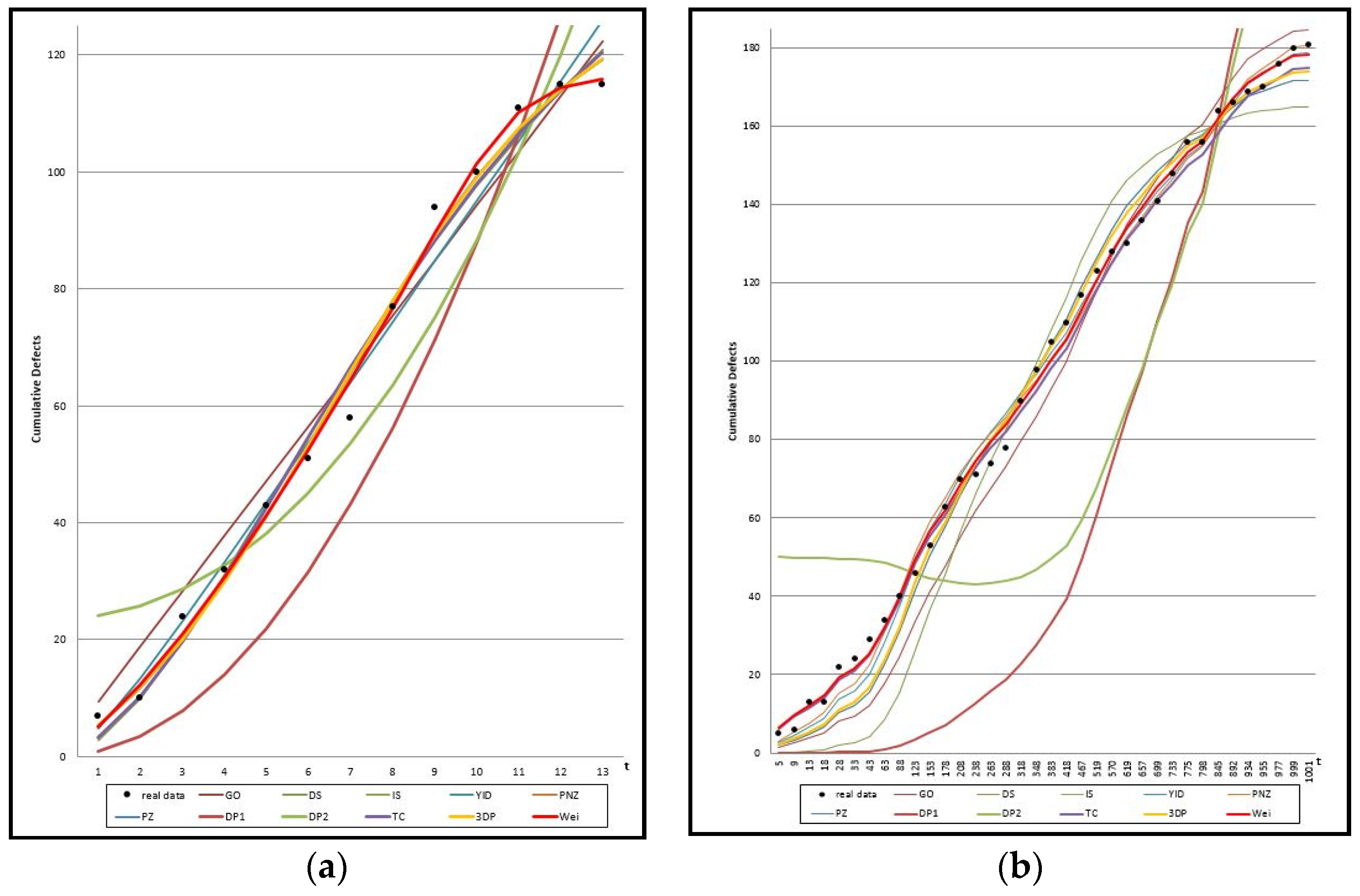
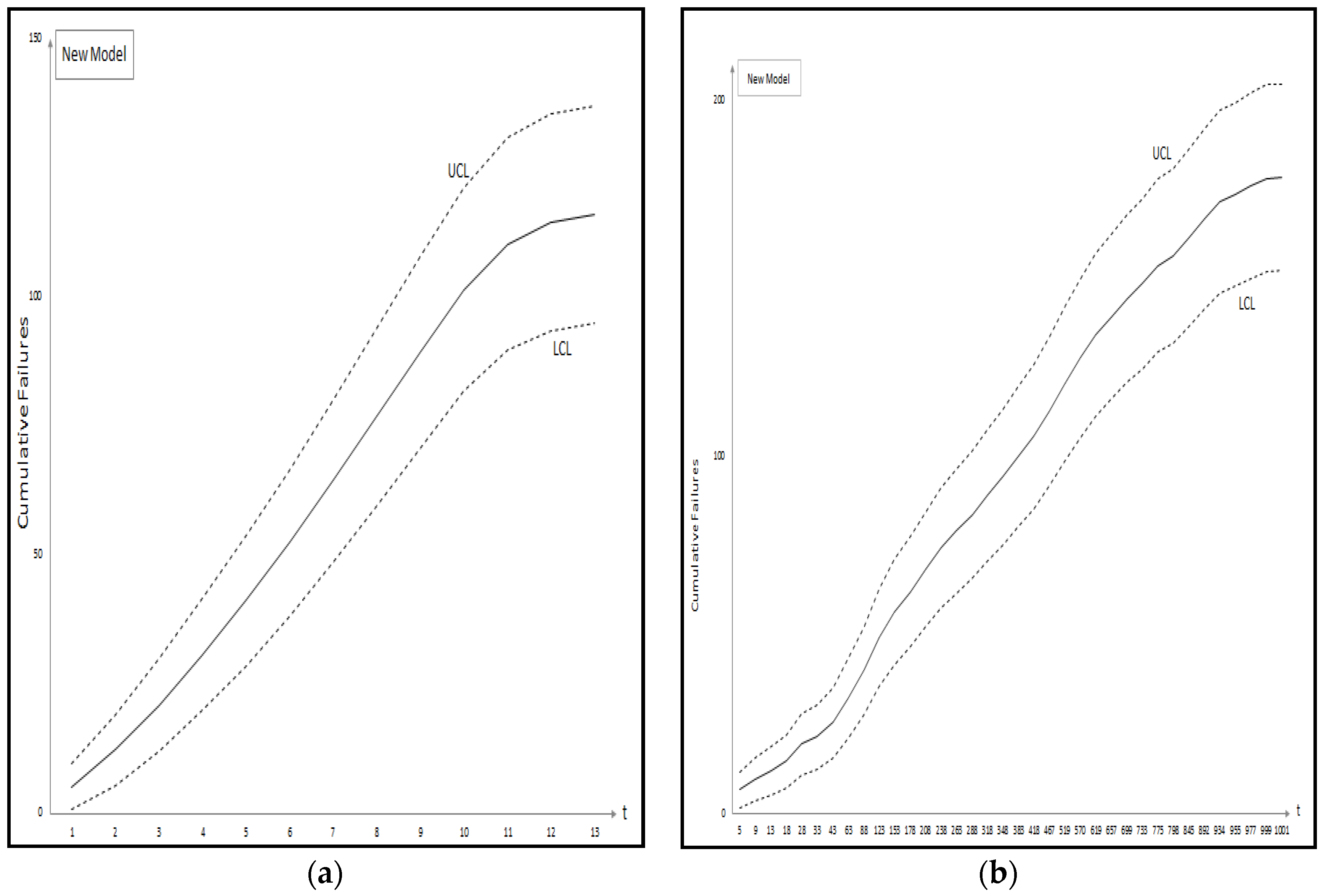
Figure 1 shows the graph of the mean value functions for all 11 models for Datasets #1 and #2, respectively. Figure 2 and Figure 3 show that the relative error value of the software reliability model can quickly approach zero in comparison with the other models confirming its ability to provide more accurate prediction. Figure 4 and Figure 5 show the graph of the mean value function and confidence interval each of the proposed new model for Datasets #1 and #2, respectively. Refer to the Appendix A for confidence intervals for the other software reliability models.
5. Conclusions
Generally, existing models are applied to software testing data and then used to make predictions on the software failures and reliability in the field. Here, the important point is that the test environment and operational environment are different from each other. We do not know in which operating environment the software will be used. Therefore, we need to develop the software reliability model considering uncertainty of operating environment. In this paper, we discussed a new software reliability model based on a Weibull fault detection rate function of Weibull distribution, which is the most commonly used distribution for modeling irregular data subject to the uncertainty of operating environments. Table 4 and Table 5 summarized the results of the estimated parameters of all 11 models in Table 1 using the LSE technique and the five common criteria (MSE, SAE, PRR, PP and AIC) value for two data sets. As can be seen from Table 4, the MSE, SAE, PRR, PP and AIC value for the proposed new model are the lowest values compared to all models. As can be seen from Table 5, the MSE, SAE and PRR value for the proposed new model are the lowest values compared to all models. As the results show the difference between the actual and predicted values of the new model is smaller than the other models, and the AIC value, which is the measure of goodness of fit of an estimated statistical model, is much smaller than the other models. Finally, we show confidence intervals of all 11 models from Dataset #1 and #2, respectively. By estimating the confidence interval, we will help to find the optimal software reliability model at different confidence levels. Future work will involve broader validation of this conclusion based on recent data sets.
Acknowledgments
This research was supported by Basic Science Research Program through the National Research Foundation of Korea (NRF) funded by the Ministry of Education (NRF-2015R1D1A1A01060050).
Author Contributions
The three authors equally contributed to the paper.
Conflicts of Interest
The authors declare no conflict of interest.
Appendix A
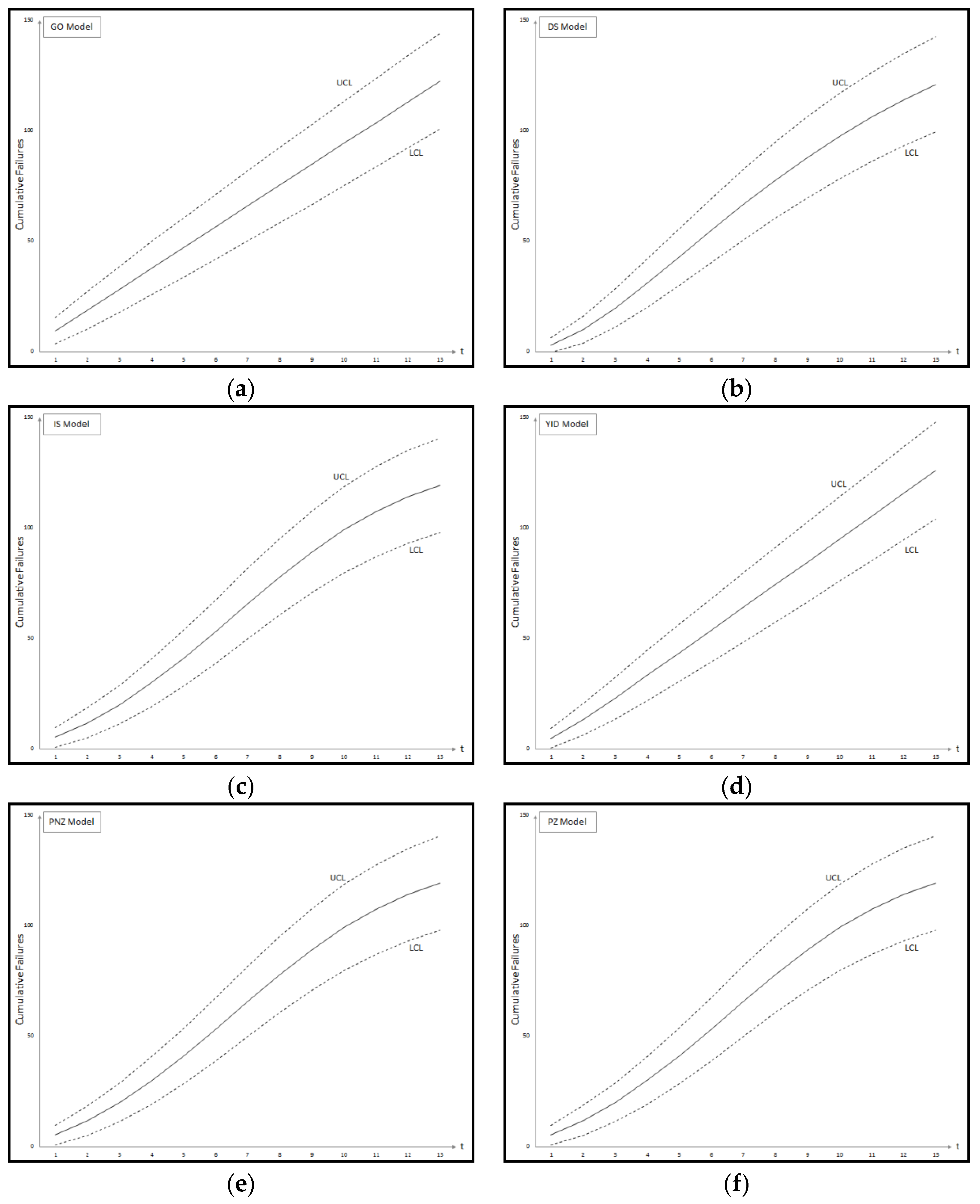
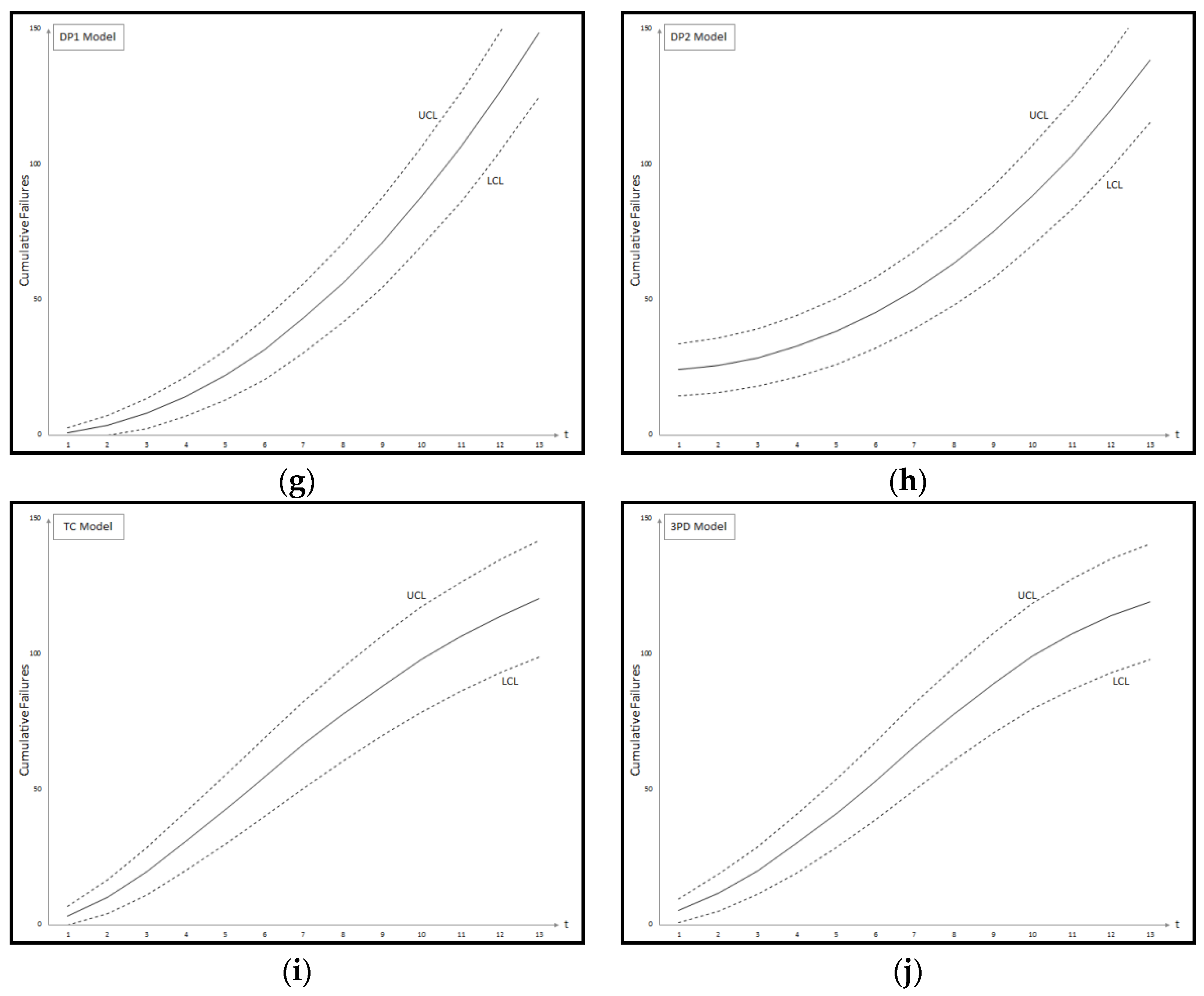
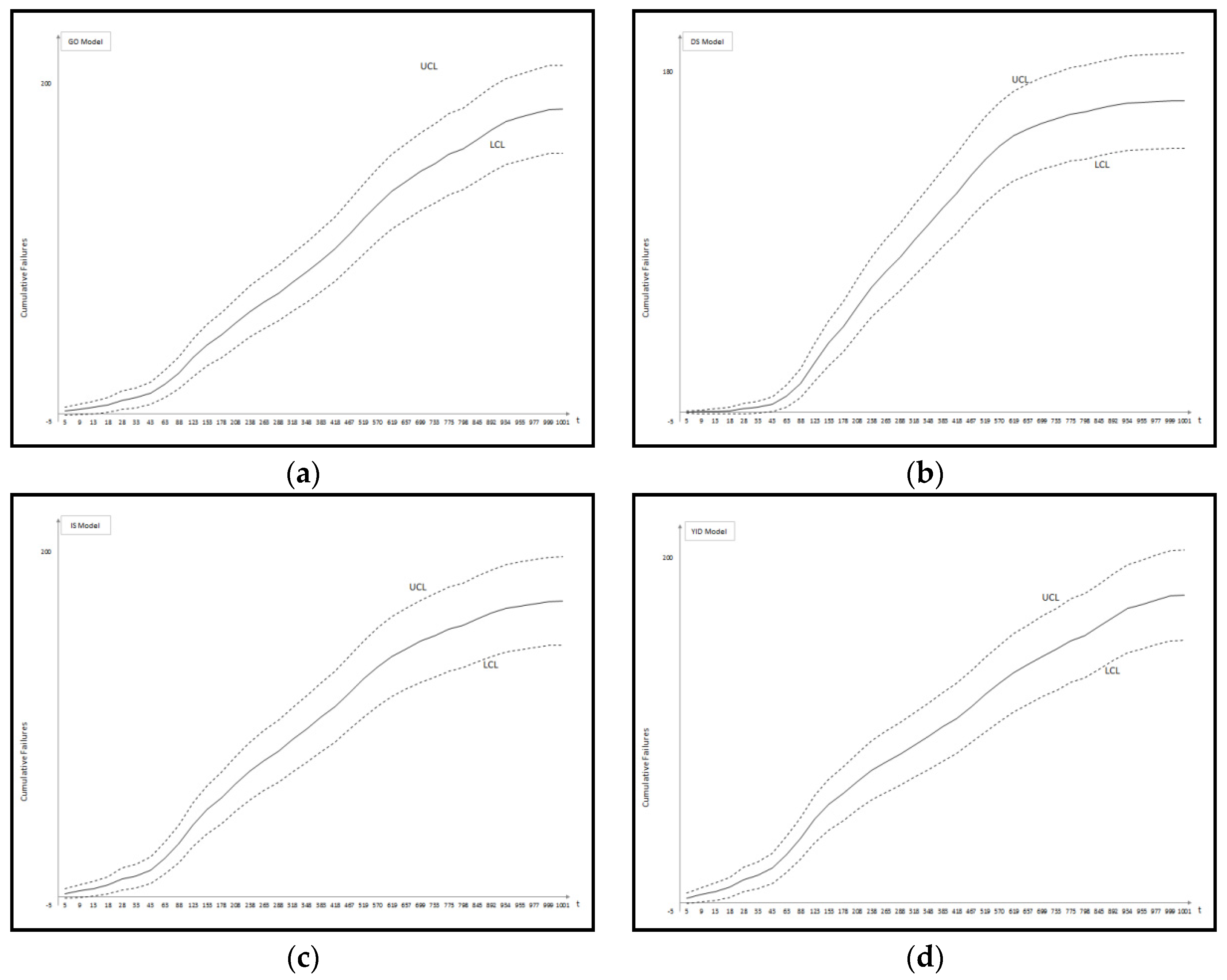
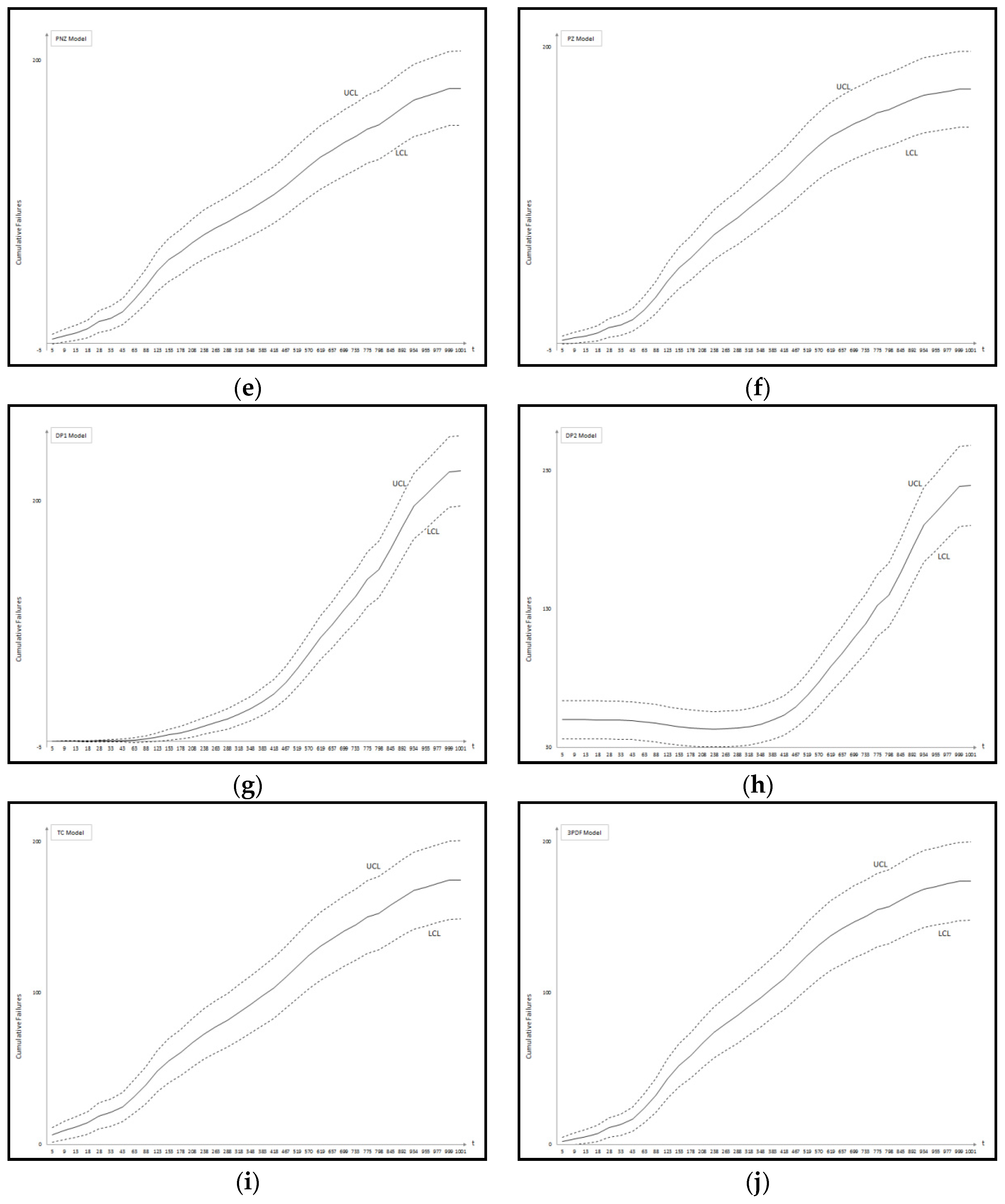
Figure A1.
Confidence intervals of all 11 models Dataset #1: (a) GO Model; (b) Delayed S-shaped SRGM; (c) Inflection S-shaped SRGM; (d) Yamada Imperfect Debugging Model; (e) PNZ Model; (f) Pham-Zhang Model; (g) Dependent-Parameter Model1; (h) Dependent-Parameter Model2; (i) Testing Coverage Model; (j) Three-parameter Model.


Figure A2.
Confidence intervals of all 11 models Dataset #2: (a) GO Model; (b) Delayed S-shaped SRGM; (c) Inflection S-shaped SRGM; (d) Yamada Imperfect Debugging Model; (e) PNZ Model; (f) Pham-Zhang Model; (g) Dependent-Parameter Model1; (h) Dependent-Parameter Model2; (i) Testing Coverage Model; (j) Three-parameter Model.


Table A1.
Confidence interval of all 11 models from Dataset #1 ().
| Time Index | 1 | 2 | 3 | 4 | 5 | 6 | 7 | 8 | 9 | 10 | 11 | 12 | 13 | |
|---|---|---|---|---|---|---|---|---|---|---|---|---|---|---|
| Model | ||||||||||||||
| GO | LCL | 3.4 | 10.3 | 17.8 | 25.6 | 33.6 | 41.8 | 50.0 | 58.3 | 66.7 | 75.1 | 83.6 | 92.2 | 100.7 |
| UCL | 15.4 | 27.3 | 38.7 | 49.7 | 60.5 | 71.2 | 81.8 | 92.3 | 102.8 | 113.2 | 123.5 | 133.8 | 144.1 | |
| DS | LCL | −0.5 | 3.7 | 11.0 | 20.0 | 30.0 | 40.3 | 50.6 | 60.4 | 69.6 | 78.1 | 86.0 | 93.0 | 99.4 |
| UCL | 6.1 | 16.1 | 28.3 | 41.8 | 55.7 | 69.4 | 82.5 | 94.9 | 106.4 | 116.9 | 126.4 | 134.9 | 142.5 | |
| IS | LCL | 0.7 | 5.1 | 11.3 | 19.1 | 28.5 | 38.9 | 49.9 | 60.7 | 70.7 | 79.6 | 87.1 | 93.1 | 97.9 |
| UCL | 9.7 | 18.6 | 28.8 | 40.6 | 53.6 | 67.5 | 81.7 | 95.3 | 107.7 | 118.6 | 127.7 | 135.0 | 140.7 | |
| YID | LCL | 0.5 | 6.2 | 13.7 | 21.9 | 30.5 | 39.4 | 48.4 | 57.5 | 66.6 | 75.9 | 85.2 | 94.6 | 104.0 |
| UCL | 9.2 | 20.5 | 32.5 | 44.5 | 56.4 | 68.1 | 79.7 | 91.3 | 102.7 | 114.1 | 125.4 | 136.7 | 147.9 | |
| PNZ | LCL | 0.7 | 5.1 | 11.3 | 19.1 | 28.5 | 38.9 | 49.9 | 60.7 | 70.7 | 79.6 | 87.1 | 93.1 | 97.9 |
| UCL | 9.7 | 18.6 | 28.8 | 40.6 | 53.6 | 67.5 | 81.6 | 95.3 | 107.7 | 118.6 | 127.7 | 135.0 | 140.7 | |
| PZ | LCL | 0.7 | 5.1 | 11.3 | 19.1 | 28.5 | 38.9 | 49.9 | 60.7 | 70.7 | 79.6 | 87.1 | 93.1 | 97.9 |
| UCL | 9.7 | 18.6 | 28.8 | 40.6 | 53.6 | 67.5 | 81.7 | 95.3 | 107.7 | 118.6 | 127.7 | 135.0 | 140.7 | |
| DP1 | LCL | −1.0 | −0.2 | 2.4 | 6.7 | 12.8 | 20.6 | 30.2 | 41.6 | 54.7 | 69.5 | 86.2 | 104.6 | 124.7 |
| UCL | 2.7 | 7.2 | 13.4 | 21.4 | 31.2 | 42.7 | 55.9 | 71.0 | 87.8 | 106.3 | 126.6 | 148.7 | 172.5 | |
| DP2 | LCL | 14.5 | 15.8 | 18.1 | 21.5 | 26.1 | 32.0 | 39.2 | 47.9 | 58.1 | 69.9 | 83.3 | 98.4 | 115.3 |
| UCL | 33.7 | 35.7 | 39.1 | 44.0 | 50.4 | 58.3 | 67.9 | 79.2 | 92.1 | 106.7 | 123.1 | 141.4 | 161.4 | |
| TC | LCL | −0.3 | 4.0 | 11.0 | 19.8 | 29.7 | 40.1 | 50.5 | 60.5 | 69.9 | 78.5 | 86.2 | 93.0 | 98.9 |
| UCL | 6.8 | 16.5 | 28.3 | 41.5 | 55.3 | 69.1 | 82.5 | 95.1 | 106.8 | 117.3 | 126.7 | 134.9 | 141.9 | |
| 3PDF | LCL | 0.7 | 5.1 | 11.3 | 19.2 | 28.5 | 38.9 | 49.9 | 60.7 | 70.7 | 79.6 | 87.1 | 93.1 | 97.9 |
| UCL | 9.7 | 18.6 | 28.8 | 40.6 | 53.6 | 67.5 | 81.7 | 95.3 | 107.7 | 118.6 | 127.7 | 135.0 | 140.7 | |
| NEW | LCL | 0.7 | 5.4 | 12.0 | 19.8 | 28.6 | 38.3 | 48.6 | 59.6 | 71.0 | 81.7 | 89.6 | 93.5 | 94.8 |
| UCL | 9.6 | 19.1 | 29.9 | 41.5 | 53.8 | 66.7 | 80.1 | 94.0 | 108.0 | 121.2 | 130.8 | 135.4 | 137.0 |
Table A2.
Confidence interval of all 11 models from Dataset #2 ().
| Time Index | 5 | 9 | 13 | 18 | 28 | 33 | 43 | 63 | 88 | 123 | 153 | 178 | |
| Model | |||||||||||||
| GO | LCL | −0.9 | −0.6 | 0.0 | 0.7 | 2.5 | 3.4 | 5.4 | 9.5 | 14.9 | 22.4 | 28.8 | 34.1 |
| UCL | 3.8 | 5.8 | 7.6 | 9.7 | 13.6 | 15.5 | 19.2 | 26.1 | 34.3 | 45.2 | 54.0 | 61.1 | |
| DS | LCL | −0.4 | −0.7 | −0.9 | −1.0 | −0.8 | −0.6 | 0.2 | 2.8 | 7.6 | 16.3 | 24.8 | 32.2 |
| UCL | 0.6 | 1.1 | 1.7 | 2.6 | 4.7 | 5.8 | 8.4 | 14.3 | 23.0 | 36.4 | 48.5 | 58.7 | |
| IS | LCL | −0.8 | −0.2 | 0.5 | 1.6 | 4.0 | 5.3 | 7.9 | 13.2 | 19.9 | 29.1 | 36.6 | 42.7 |
| UCL | 4.6 | 7.0 | 9.2 | 11.8 | 16.6 | 18.9 | 23.4 | 31.8 | 41.6 | 54.4 | 64.5 | 72.4 | |
| YID | LCL | −0.6 | 0.4 | 1.5 | 3.1 | 6.3 | 8.0 | 11.3 | 17.7 | 25.3 | 34.9 | 42.2 | 47.8 |
| UCL | 5.7 | 8.7 | 11.5 | 14.8 | 20.7 | 23.5 | 28.9 | 38.5 | 49.2 | 62.2 | 71.8 | 79.0 | |
| PNZ | LCL | −0.4 | 0.8 | 2.1 | 4.0 | 7.7 | 9.5 | 13.2 | 20.1 | 27.8 | 37.1 | 44.0 | 49.2 |
| UCL | 6.3 | 9.8 | 12.9 | 16.5 | 23.1 | 26.1 | 31.8 | 41.9 | 52.6 | 65.2 | 74.2 | 80.8 | |
| PZ | LCL | −0.8 | −0.2 | 0.5 | 1.6 | 4.0 | 5.3 | 7.9 | 13.2 | 19.9 | 29.1 | 36.6 | 42.7 |
| UCL | 4.6 | 7.0 | 9.2 | 11.8 | 16.6 | 18.9 | 23.4 | 31.8 | 41.7 | 54.4 | 64.5 | 72.5 | |
| DP1 | LCL | −0.1 | −0.2 | −0.3 | −0.5 | −0.7 | −0.7 | −0.9 | −1.0 | −0.8 | −0.2 | 0.8 | 1.9 |
| UCL | 0.2 | 0.3 | 0.4 | 0.6 | 1.0 | 1.2 | 1.7 | 2.7 | 4.3 | 7.0 | 9.8 | 12.4 | |
| DP2 | LCL | 36.1 | 36.1 | 36.0 | 36.0 | 35.8 | 35.7 | 35.5 | 34.8 | 33.9 | 32.6 | 31.6 | 30.9 |
| UCL | 63.8 | 63.8 | 63.7 | 63.7 | 63.4 | 63.3 | 63.0 | 62.1 | 60.9 | 59.2 | 57.8 | 56.9 | |
| TC | LCL | 1.3 | 3.2 | 4.9 | 6.8 | 10.3 | 12.0 | 15.0 | 20.6 | 26.8 | 34.6 | 40.8 | 45.6 |
| UCL | 11.1 | 15.0 | 18.2 | 21.6 | 27.4 | 29.9 | 34.5 | 42.6 | 51.3 | 61.9 | 69.9 | 76.2 | |
| 3PDF | LCL | −0.8 | −0.1 | 0.8 | 2.0 | 4.6 | 5.9 | 8.7 | 14.3 | 21.2 | 30.5 | 38.0 | 43.9 |
| UCL | 4.9 | 7.4 | 9.8 | 12.5 | 17.6 | 20.1 | 24.7 | 33.5 | 43.5 | 56.3 | 66.3 | 74.0 | |
| NEW | LCL | 1.5 | 3.4 | 5.1 | 7.1 | 10.7 | 12.4 | 15.5 | 21.1 | 27.5 | 35.4 | 41.7 | 46.6 |
| UCL | 11.5 | 15.4 | 18.7 | 22.1 | 27.9 | 30.5 | 35.2 | 43.4 | 52.2 | 62.9 | 71.1 | 77.5 | |
| Time Index | 208 | 238 | 263 | 288 | 318 | 348 | 383 | 418 | 467 | 519 | 570 | 619 | |
| Model | |||||||||||||
| GO | LCL | 40.3 | 46.4 | 51.4 | 56.3 | 62.0 | 67.6 | 74.0 | 80.1 | 88.4 | 96.8 | 104.7 | 111.9 |
| UCL | 69.3 | 77.2 | 83.6 | 89.8 | 97.0 | 103.9 | 111.7 | 119.3 | 129.3 | 139.4 | 148.8 | 157.4 | |
| DS | LCL | 41.3 | 50.3 | 57.6 | 64.6 | 72.5 | 79.8 | 87.7 | 94.8 | 103.5 | 111.3 | 117.5 | 122.5 |
| UCL | 70.7 | 82.2 | 91.4 | 100.1 | 109.9 | 118.9 | 128.5 | 137.0 | 147.4 | 156.6 | 164.0 | 169.9 | |
| IS | LCL | 49.7 | 56.4 | 61.7 | 66.8 | 72.6 | 78.1 | 84.2 | 89.9 | 97.4 | 104.5 | 110.9 | 116.5 |
| UCL | 81.4 | 89.9 | 96.5 | 102.9 | 110.1 | 116.8 | 124.2 | 131.2 | 140.1 | 148.7 | 156.2 | 162.9 | |
| YID | LCL | 54.0 | 59.7 | 64.1 | 68.2 | 72.9 | 77.3 | 82.2 | 86.9 | 93.1 | 99.4 | 105.3 | 110.9 |
| UCL | 86.9 | 94.0 | 99.5 | 104.7 | 110.5 | 115.9 | 121.8 | 127.5 | 135.0 | 142.5 | 149.6 | 156.2 | |
| PNZ | LCL | 54.8 | 59.9 | 63.8 | 67.6 | 71.9 | 75.9 | 80.5 | 85.0 | 91.0 | 97.3 | 103.4 | 109.2 |
| UCL | 87.9 | 94.3 | 99.2 | 103.9 | 109.1 | 114.1 | 119.7 | 125.1 | 132.5 | 140.0 | 147.3 | 154.2 | |
| PZ | LCL | 49.7 | 56.4 | 61.7 | 66.8 | 72.6 | 78.1 | 84.2 | 90.0 | 97.4 | 104.6 | 110.9 | 116.5 |
| UCL | 81.5 | 89.9 | 96.6 | 102.9 | 110.1 | 116.9 | 124.3 | 131.2 | 140.1 | 148.7 | 156.3 | 162.9 | |
| DP1 | LCL | 3.6 | 5.8 | 7.8 | 10.2 | 13.4 | 17.0 | 21.7 | 27.0 | 35.3 | 45.3 | 56.3 | 68.0 |
| UCL | 15.9 | 19.7 | 23.3 | 27.1 | 32.1 | 37.5 | 44.3 | 51.6 | 62.8 | 75.9 | 89.9 | 104.4 | |
| DP2 | LCL | 30.4 | 30.2 | 30.4 | 30.8 | 31.8 | 33.3 | 35.7 | 38.7 | 44.2 | 51.5 | 60.2 | 70.0 |
| UCL | 56.2 | 55.9 | 56.2 | 56.8 | 58.1 | 60.1 | 63.2 | 67.3 | 74.4 | 83.8 | 94.8 | 106.9 | |
| TC | LCL | 51.0 | 56.2 | 60.4 | 64.4 | 69.0 | 73.5 | 78.5 | 83.4 | 89.9 | 96.6 | 102.9 | 108.7 |
| UCL | 83.1 | 89.7 | 94.9 | 99.9 | 105.6 | 111.1 | 117.3 | 123.2 | 131.1 | 139.2 | 146.7 | 153.6 | |
| 3PDF | LCL | 50.7 | 57.1 | 62.2 | 67.0 | 72.5 | 77.8 | 83.5 | 89.0 | 96.1 | 103.0 | 109.3 | 115.0 |
| UCL | 82.7 | 90.8 | 97.1 | 103.2 | 110.0 | 116.4 | 123.4 | 130.0 | 138.6 | 146.9 | 154.4 | 161.0 | |
| NEW | LCL | 52.2 | 57.5 | 61.8 | 65.9 | 70.7 | 75.3 | 80.4 | 85.5 | 92.2 | 99.1 | 105.5 | 111.5 |
| UCL | 84.6 | 91.3 | 96.7 | 101.8 | 107.7 | 113.3 | 119.7 | 125.7 | 133.9 | 142.1 | 149.8 | 156.9 | |
| Time Index | 657 | 699 | 733 | 775 | 798 | 845 | 892 | 934 | 955 | 977 | 999 | 1001 | |
| Model | |||||||||||||
| GO | LCL | 117.3 | 123.0 | 127.5 | 132.8 | 135.6 | 141.2 | 146.5 | 151.0 | 153.2 | 155.5 | 157.7 | 157.9 |
| UCL | 163.8 | 170.5 | 175.7 | 181.9 | 185.2 | 191.7 | 197.9 | 203.2 | 205.8 | 208.4 | 210.9 | 211.2 | |
| DS | LCL | 125.7 | 128.7 | 130.8 | 133.0 | 134.0 | 135.8 | 137.3 | 138.3 | 138.8 | 139.2 | 139.6 | 139.7 |
| UCL | 173.6 | 177.2 | 179.6 | 182.2 | 183.4 | 185.5 | 187.2 | 188.4 | 189.0 | 189.5 | 189.9 | 190.0 | |
| IS | LCL | 120.5 | 124.6 | 127.7 | 131.2 | 133.1 | 136.5 | 139.7 | 142.3 | 143.5 | 144.8 | 145.9 | 146.0 |
| UCL | 167.6 | 172.4 | 176.0 | 180.1 | 182.3 | 186.3 | 190.0 | 193.1 | 194.5 | 195.9 | 197.3 | 197.4 | |
| YID | LCL | 115.1 | 119.8 | 123.5 | 128.1 | 130.6 | 135.6 | 140.7 | 145.2 | 147.5 | 149.8 | 152.2 | 152.4 |
| UCL | 161.2 | 166.7 | 171.1 | 176.5 | 179.4 | 185.3 | 191.2 | 196.4 | 199.1 | 201.8 | 204.5 | 204.8 | |
| PNZ | LCL | 113.7 | 118.7 | 122.7 | 127.6 | 130.3 | 135.9 | 141.4 | 146.4 | 148.9 | 151.5 | 154.1 | 154.3 |
| UCL | 159.5 | 165.4 | 170.1 | 175.9 | 179.1 | 185.6 | 192.0 | 197.8 | 200.7 | 203.7 | 206.7 | 207.0 | |
| PZ | LCL | 120.5 | 124.6 | 127.7 | 131.2 | 133.0 | 136.5 | 139.7 | 142.3 | 143.5 | 144.7 | 145.9 | 146.0 |
| UCL | 167.6 | 172.4 | 176.0 | 180.1 | 182.3 | 186.3 | 190.0 | 193.0 | 194.5 | 195.9 | 197.3 | 197.4 | |
| DP1 | LCL | 77.8 | 89.4 | 99.3 | 112.4 | 119.8 | 135.8 | 152.8 | 168.8 | 177.1 | 186.0 | 195.2 | 196.0 |
| UCL | 116.4 | 130.5 | 142.4 | 157.9 | 166.7 | 185.5 | 205.2 | 223.7 | 233.3 | 243.5 | 253.9 | 254.9 | |
| DP2 | LCL | 78.5 | 88.9 | 98.0 | 110.0 | 117.0 | 132.2 | 148.5 | 164.1 | 172.1 | 180.9 | 189.8 | 190.6 |
| UCL | 117.3 | 129.9 | 140.8 | 155.2 | 163.5 | 181.3 | 200.3 | 218.2 | 227.6 | 237.5 | 247.8 | 248.7 | |
| TC | LCL | 113.1 | 117.8 | 121.6 | 126.1 | 128.5 | 133.4 | 138.2 | 142.3 | 144.4 | 146.5 | 148.6 | 148.8 |
| UCL | 158.8 | 164.4 | 168.8 | 174.1 | 177.0 | 182.7 | 188.2 | 193.1 | 195.5 | 198.0 | 200.4 | 200.6 | |
| 3PDF | LCL | 119.1 | 123.3 | 126.6 | 130.5 | 132.5 | 136.4 | 140.2 | 143.3 | 144.8 | 146.4 | 147.9 | 148.0 |
| UCL | 165.8 | 170.9 | 174.7 | 179.2 | 181.6 | 186.2 | 190.6 | 194.3 | 196.0 | 197.8 | 199.6 | 199.7 | |
| NEW | LCL | 116.0 | 120.8 | 124.6 | 129.2 | 131.7 | 136.6 | 141.4 | 145.6 | 147.7 | 149.8 | 151.9 | 152.1 |
| UCL | 162.2 | 167.9 | 172.4 | 177.8 | 180.7 | 186.4 | 192.1 | 196.9 | 199.3 | 201.8 | 204.2 | 204.5 |
References
- Fang, C.C.; Yeh, C.W. Confidence interval estimation of software reliability growth models derived from stochastic differential equations. In Proceedings of the IEEE International Conference on Industrial Engineering and Engineering Management (IEEM), Singapore, 6–9 December 2011; pp. 1843–1847. [Google Scholar]
- Yamada, S.; Osaki, S. Software reliability growth modeling: Models and applications. IEEE Trans. Softw. Eng. 1985, 11, 1431–1437. [Google Scholar] [CrossRef]
- Yin, L.; Trivedi, K.S. Confidence interval estimation of NHPP-based software reliability models. In Proceedings of the 10th International Symposium on Software Reliability Engineering, Boca Raton, FL, USA, 1–4 November 1999; pp. 6–11. [Google Scholar]
- Huang, C.Y. Performance analysis of software reliability growth models with testing effort and change-point. J. Syst. Softw. 2005, 76, 181–194. [Google Scholar] [CrossRef]
- Gonzalez, C.A.; Torres, A.; Rios, M.A. Reliability assessment of distribution power repairable systems using NHPP. In Proceedings of the 2014 IEEE PES Transmission & Distribution Conference and Exposition-Latin America (PES T&D-LA), Medellin, Colombia, 10–13 September 2014; pp. 1–6. [Google Scholar]
- Nagaraju, V.; Fiondella, L. An adaptive EM algorithm for NHPP software reliability models. In Proceedings of the 2015 Annual Reliability and Maintainability Symposium (RAMS), Palm Harbor, FL, USA, 26–29 January 2015; pp. 1–6. [Google Scholar]
- Srivastava, N.K.; Mondal, S. Development of predictive maintenance model for N-component repairable system using NHPP models and system availability concept. Glob. Bus. Rev. 2016, 17, 105–115. [Google Scholar] [CrossRef]
- Kim, K.C.; Kim, Y.H.; Shin, J.H.; Han, K.J. A Case Study on Application for Software Reliability Model to Improve Reliability of the Weapon System. J. KIISE 2011, 38, 405–418. [Google Scholar]
- Chatterjee, S.; Singh, J.B. A NHPP based software reliability model and optimal release policy with logistic-exponential test coverage under imperfect debugging. Int. J. Syst. Assur. Eng. Manag. 2014, 5, 399–406. [Google Scholar] [CrossRef]
- Chatterjee, S.; Shulka, A. Software reliability modeling with different type of faults incorporating both imperfect debugging and change point. In Proceedings of the 4th International Conference on Reliability, Infocom, Technologies and Optimization, Noida, India, 2–4 September 2015; pp. 1–5. [Google Scholar]
- Yamada, S.; Hishitani, J.; Osaki, S. Software-reliability growth with a Weibull test-effort: A model and application. IEEE Trans. Reliab. 1993, 42, 100–106. [Google Scholar] [CrossRef]
- Joh, H.C.; Kim, J.; Malaiya, Y.K. FAST ABSTRACT: Vulnerability discovery modelling using Weibull distribution. In Proceedings of the 19th International Symposium on Software Reliability Engineering, Seattle, WA, USA, 10–14 November 2008; pp. 299–300. [Google Scholar]
- Sagar, B.B.; Saket, R.K.; Singh, C.G. Exponentiated Weibull distribution approach based inflection S-shaped software reliability growth model. Ain Shams Eng. J. 2016, 7, 973–991. [Google Scholar] [CrossRef]
- Yang, B.; Xie, M. A study of operational and testing reliability in software reliability analysis. Reliab. Eng. Syst. Saf. 2000, 70, 323–329. [Google Scholar] [CrossRef]
- Huang, C.Y.; Kuo, S.Y.; Lyu, M.R.; Lo, J.H. Quantitative software reliability modeling from testing from testing to operation. In Proceedings of the International Symposium on Software Reliability Engineering, Los Alamitos, CA, USA, 8–11 October 2000; pp. 72–82. [Google Scholar]
- Zhang, X.; Jeske, D.; Pham, H. Calibrating software reliability models when the test environment does not match the user environment. Appl. Stoch. Models Bus. Ind. 2002, 18, 87–99. [Google Scholar] [CrossRef]
- Teng, X.; Pham, H. A new methodology for predicting software reliability in the random field environments. IEEE Trans. Reliab. 2006, 55, 458–468. [Google Scholar] [CrossRef]
- Pham, H. A software reliability model with Vtub-Shaped fault-detection rate subject to operating environments. In Proceedings of the 19th ISSAT International Conference on Reliability and Quality in Design, Honolulu, HI, USA, 5–7 August 2013; pp. 33–37. [Google Scholar]
- Pham, H. A new software reliability model with Vtub-Shaped fault detection rate and the uncertainty of operating environments. Optimization 2014, 63, 1481–1490. [Google Scholar] [CrossRef]
- Chang, I.H.; Pham, H.; Lee, S.W.; Song, K.Y. A testing-coverage software reliability model with the uncertainty of operation environments. Int. J. Syst. Sci. Oper. Logist. 2014, 1, 220–227. [Google Scholar]
- Honda, K.; Nakai, H.; Washizaki, H.; Fukazawa, Y. Predicting time range of development based on generalized software reliability model. In Proceedings of the 21st Asia-Pacific Software Engineering Conference, Jeju, Korea, 1–4 December 2014; pp. 351–358. [Google Scholar]
- Pham, H. A generalized fault-detection software reliability model subject to random operating environments. Vietnam J. Comp. Sci. 2016, 3, 145–150. [Google Scholar] [CrossRef]
- Song, K.Y.; Chang, I.H.; Pham, H. A Three-parameter fault-detection software reliability model with the uncertainty of operating environments. J. Syst. Sci. Syst. Eng. 2017, 26, 121–132. [Google Scholar] [CrossRef]
- Pham, H.; Nordmann, L.; Zhang, X. A general imperfect software debugging model with S-shaped fault detection rate. IEEE Trans. Reliab. 1999, 48, 169–175. [Google Scholar] [CrossRef]
- Gupta, R.D.; Kundu, D. Exponentiated exponential family: An alternative to gamma and Weibull distributions. Biom. J. 2001, 43, 117–130. [Google Scholar] [CrossRef]
- Huo, Y.; Jing, T.; Li, S. Dual parameter Weibull distribution-based rate distortion model. In Proceedings of the International Conference on Computational Intelligence and Software Engineering, Wuhan, China, 11–13 December 2009; pp. 1–4. [Google Scholar]
- Pham, H. System Software Reliability; Springer: London, UK, 2006. [Google Scholar]
- Akaike, H. A new look at statistical model identification. IEEE Trans. Autom. Control 1974, 19, 716–719. [Google Scholar] [CrossRef]
- Goel, A.L.; Okumoto, K. Time dependent error detection rate model for software reliability and other performance measures. IEEE Trans. Reliab. 1979, 28, 206–211. [Google Scholar] [CrossRef]
- Yamada, S.; Ohba, M.; Osaki, S. S-shaped reliability growth modeling for software fault detection. IEEE Trans. Reliab. 1983, 32, 475–484. [Google Scholar] [CrossRef]
- Ohba, M. Inflexion S-shaped software reliability growth models. In Stochastic Models in Reliability Theory; Osaki, S., Hatoyama, Y., Eds.; Springer: Berlin, Germany, 1984; pp. 144–162. [Google Scholar]
- Yamada, S.; Tokuno, K.; Osaki, S. Imperfect debugging models with fault introduction rate for software reliability assessment. Int. J. Syst. Sci. 1992, 23, 2241–2252. [Google Scholar] [CrossRef]
- Pham, H.; Zhang, X. An NHPP software reliability models and its comparison. Int. J. Reliab. Qual. Saf. Eng. 1997, 4, 269–282. [Google Scholar] [CrossRef]
- Pham, H. Software Reliability Models with Time Dependent Hazard Function Based on Bayesian Approach. Int. J. Autom. Comput. 2007, 4, 325–328. [Google Scholar] [CrossRef]
- Jeske, D.R.; Zhang, X. Some successful approaches to software reliability modeling in industry. J. Syst. Softw. 2005, 74, 85–99. [Google Scholar] [CrossRef]
Figure 1.
Mean value function of all 11 models; (a) Dataset #1; (b) Dataset #2.

Figure 2.
Relative error value of 11 models in Table 1 for Dataset #1.
Figure 2.
Relative error value of 11 models in Table 1 for Dataset #1.
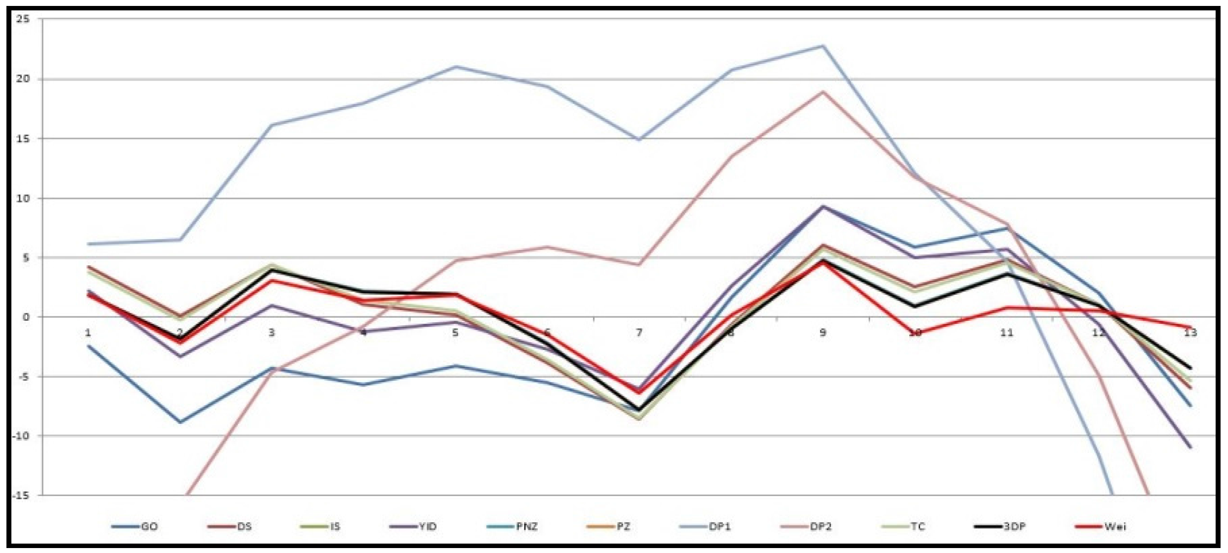
Figure 3.
Relative error value of 11 models in Table 1 for Dataset #2.
Figure 3.
Relative error value of 11 models in Table 1 for Dataset #2.
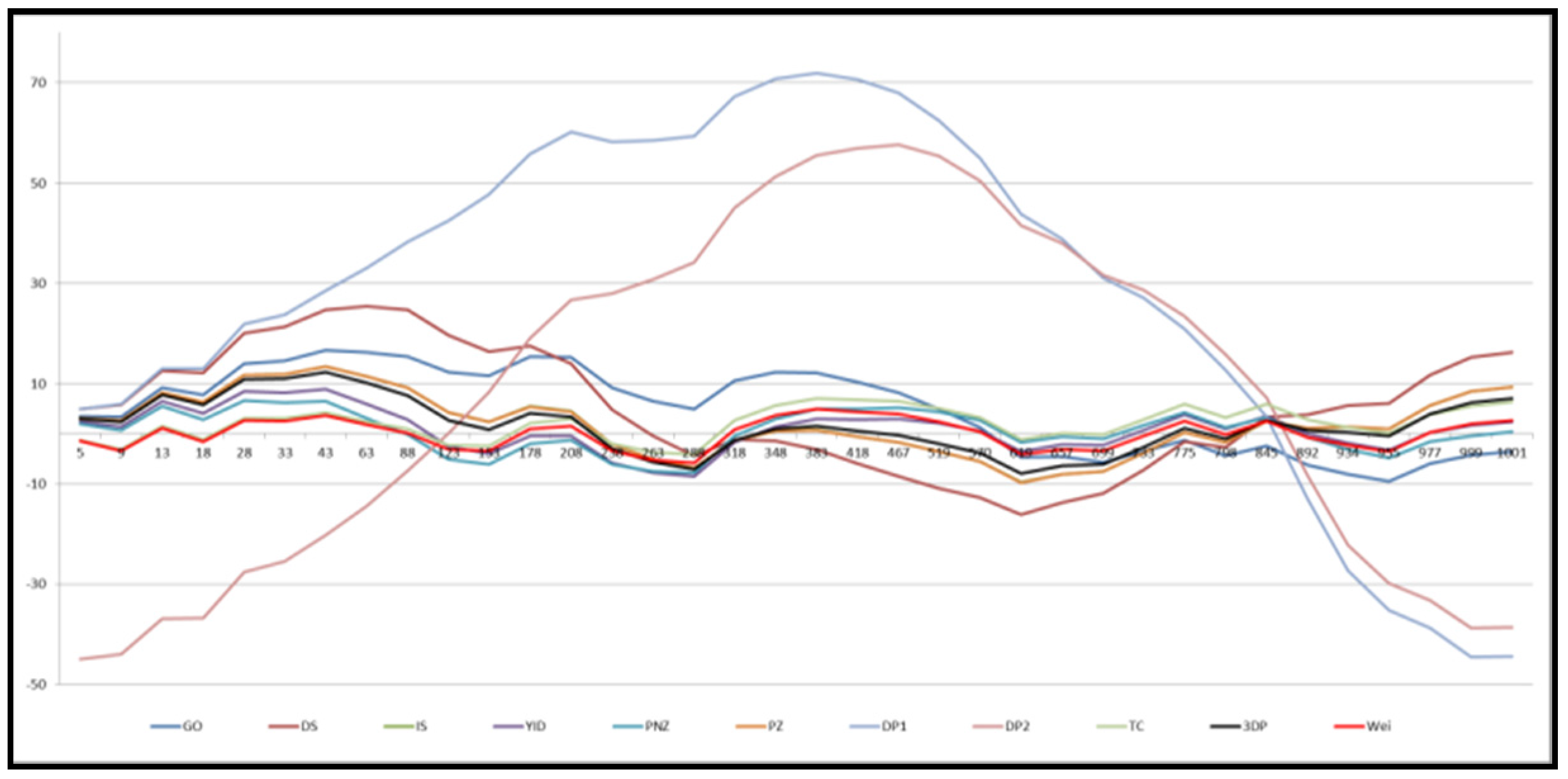
Figure 4.
Confidence intervals of the proposed new model; (a) Dataset #1; (b) Dataset #2.

Table 1.
Software reliability models. Software reliability growth model (SRGM).
| No. | Model | |
|---|---|---|
| 1 | G-O Model [29] | |
| 2 | Delayed S-shaped SRGM [30] | |
| 3 | Inflection S-shaped SRGM [31] | |
| 4 | Yamada Imperfect Debugging Model [32] | |
| 5 | PNZ Model [24] | |
| 6 | Pham-Zhang Model [33] | |
| 7 | Dependent-Parameter Model1 [34] | |
| 8 | Dependent-Parameter Model2 [34] | |
| 9 | Testing Coverage Model [20] | |
| 10 | Three-parameter Model [23] | |
| 11 | Proposed New Model |
Table 2.
Field failure data for Release 1—Dataset #1.
| Month Index | System Days (Days) | System Days (Cumulative) | Failures | Cumulative Failures |
|---|---|---|---|---|
| 1 | 961 | 961 | 7 | 7 |
| 2 | 4170 | 5131 | 3 | 10 |
| 3 | 8789 | 13,920 | 14 | 24 |
| 4 | 11,858 | 25,778 | 8 | 32 |
| 5 | 13,110 | 38,888 | 11 | 43 |
| 6 | 14,198 | 53,086 | 8 | 51 |
| 7 | 14,265 | 67,351 | 7 | 58 |
| 8 | 15,175 | 82,526 | 19 | 77 |
| 9 | 15,376 | 97,902 | 17 | 94 |
| 10 | 15,704 | 113,606 | 6 | 100 |
| 11 | 18,182 | 131,788 | 11 | 111 |
| 12 | 17,760 | 149,548 | 4 | 115 |
| 13 | 18,352 | 167,900 | 0 | 115 |
Table 3.
Test data for Release 2—Dataset #2.
| Week Index | System Days (Cumulative) | Cumulative Failures | Week Index | System Days (Cumulative) | Cumulative Failures |
|---|---|---|---|---|---|
| 1 | 5 | 5 | 19 | 383 | 105 |
| 2 | 9 | 6 | 20 | 418 | 110 |
| 3 | 13 | 13 | 21 | 467 | 117 |
| 4 | 18 | 13 | 22 | 519 | 123 |
| 5 | 28 | 22 | 23 | 570 | 128 |
| 6 | 33 | 24 | 24 | 619 | 130 |
| 7 | 43 | 29 | 25 | 657 | 136 |
| 8 | 63 | 34 | 26 | 699 | 141 |
| 9 | 88 | 40 | 27 | 733 | 148 |
| 10 | 123 | 46 | 28 | 775 | 156 |
| 11 | 153 | 53 | 29 | 798 | 156 |
| 12 | 178 | 63 | 30 | 845 | 164 |
| 13 | 203 | 70 | 31 | 892 | 166 |
| 14 | 238 | 71 | 32 | 934 | 169 |
| 15 | 263 | 74 | 33 | 955 | 170 |
| 16 | 288 | 78 | 34 | 977 | 176 |
| 17 | 318 | 90 | 35 | 999 | 180 |
| 18 | 348 | 98 | 36 | 1001 | 181 |
Table 4.
Model parameter estimation and comparison criteria from Dataset #1. Least-squares estimate (LSE); mean squared error (MSE); sum absolute error (SAE); predictive ratio risk (PRR), predictive power (PP); Akaike’s information criterion (AIC).
Table 4.
Model parameter estimation and comparison criteria from Dataset #1. Least-squares estimate (LSE); mean squared error (MSE); sum absolute error (SAE); predictive ratio risk (PRR), predictive power (PP); Akaike’s information criterion (AIC).
| Model | LSE’s | MSE | SAE | PRR | PP | AIC |
|---|---|---|---|---|---|---|
| GO | = 2354138, = 0.000004 | 43.6400 | 72.2548 | 0.3879 | 1.0239 | 98.7606 |
| DS | = 168.009, = 0.195 | 20.7414 | 43.2510 | 2.3107 | 0.4295 | 92.2587 |
| IS | = 134.540, = 0.336, = 8.939 | 15.3196 | 37.2090 | 0.2120 | 0.1587 | 85.3000 |
| YID | = 1.130, = 1.110, = 9.129 | 33.3890 | 51.0913 | 0.3027 | 0.2495 | 100.7378 |
| PNZ | = 134.549, = 0.3359, = 0.0, = 8.940 | 17.0223 | 37.2442 | 0.2124 | 0.1588 | 87.3098 |
| PZ | = 51.455, = 0.336, = 289998.1, = 8.939, = 83.085 | 19.1495 | 37.2091 | 0.2120 | 0.1587 | 89.3019 |
| DP1 | = 0.0088, = 9.996 | 370.8651 | 207.3750 | 60.5062 | 2.6446 | 164.5728 |
| DP2 | = 672.637, = 0.04, = 0.027, = 23.541 | 215.7784 | 133.2294 | 1.1037 | 8.6260 | 168.846 |
| TC | = 0.242, = 1.701, = 17.967, = 73.604, = 149.410 | 25.9244 | 41.8087 | 1.4473 | 0.3601 | 95.5655 |
| 3DP | = 2.980, = 0.336, = 0.080, = 1105.772, = 135.142 | 19.1517 | 37.2107 | 0.2119 | 0.1588 | 89.3053 |
| NEW | = 0.095, = 15.606, = 0.085, = 1.855, = 116.551 | 11.2281 | 26.5568 | 0.2042 | 0.1558 | 79.3459 |
Table 5.
Model parameter estimation and comparison criteria from Dataset #2.
| Model | LSE’s | MSE | SAE | PRR | PP | AIC |
|---|---|---|---|---|---|---|
| GO | = 291.768, = 0.001 | 95.3796 | 299.7160 | 24.7924 | 3.4879 | 198.5419 |
| DS | = 168.568, = 0.0057 | 178.4899 | 387.7724 | 7368.5885 | 7.4923 | 317.8791 |
| IS | = 200.110, = 0.002, = 0.059 | 43.2888 | 182.9709 | 10.4336 | 2.1725 | 202.0752 |
| YID | = 81.999, = 0.0063, = 0.0014 | 18.9651 | 119.1208 | 3.1804 | 1.0871 | 187.7564 |
| PNZ | = 67.132, = 0.009, = 0.0019, = 0.0001 | 18.2406 | 119.7722 | 1.5566 | 0.6869 | 188.9438 |
| PZ | = 200.057, = 0.002, = 9999.433, = 0.058, = 0.001 | 46.0819 | 183.0449 | 10.4090 | 2.1698 | 206.0887 |
| DP1 | = 0.0003, = 0.866 | 2075.6677 | 1411.8412 | 1,165,906.40 | 17.1338 | 554.6335 |
| DP2 | = 9.035, = 0.005, = 48.975, = 49.004 | 1379.2331 | 1134.6843 | 13.0318 | 156.8519 | 572.8343 |
| TC | = 0.002, = 0.646, = 0.137, = 8.920, = 7973.501 | 16.5529 | 116.0937 | 0.3033 | 0.4499 | 187.4100 |
| 3DP | = 0.011, = 0.707, = 8.029, = 0.000001, = 300.684 | 34.5762 | 154.1593 | 7.7768 | 1.8500 | 199.3282 |
| NEW | = 0.004, = 1.471, = 0.430, = 78.738, = 504.403 | 9.8789 | 90.3633 | 0.2944 | 0.5159 | 187.4204 |
© 2017 by the authors. Licensee MDPI, Basel, Switzerland. This article is an open access article distributed under the terms and conditions of the Creative Commons Attribution (CC BY) license (http://creativecommons.org/licenses/by/4.0/).
Share and Cite
MDPI and ACS Style
Song, K.Y.; Chang, I.H.; Pham, H. A Software Reliability Model with a Weibull Fault Detection Rate Function Subject to Operating Environments. Appl. Sci. 2017, 7, 983. https://doi.org/10.3390/app7100983
AMA Style
Song KY, Chang IH, Pham H. A Software Reliability Model with a Weibull Fault Detection Rate Function Subject to Operating Environments. Applied Sciences. 2017; 7(10):983. https://doi.org/10.3390/app7100983
Chicago/Turabian StyleSong, Kwang Yoon, In Hong Chang, and Hoang Pham. 2017. "A Software Reliability Model with a Weibull Fault Detection Rate Function Subject to Operating Environments" Applied Sciences 7, no. 10: 983. https://doi.org/10.3390/app7100983
Note that from the first issue of 2016, this journal uses article numbers instead of page numbers. See further details here.