Classification of Architectural Heritage Images Using Deep Learning Techniques
by
 ,
,
Jose Llamas
1,* ,
,
Pedro M. Lerones
1,
Roberto Medina
1,
Eduardo Zalama
2 and
Jaime Gómez-García-Bermejo
2
1
CARTIF Foundation, Parque Tecnológico de Boecillo, 47151 Valladolid, Spain
2
ITAP-DISA, University of Valladolid, Pl. Santa Cruz, 8, 47002 Valladolid, Spain
*
Author to whom correspondence should be addressed.
Appl. Sci. 2017, 7(10), 992; https://doi.org/10.3390/app7100992
Submission received: 7 September 2017
/
Revised: 21 September 2017
/
Accepted: 21 September 2017
/
Published: 26 September 2017
Abstract
:The classification of the images taken during the measurement of an architectural asset is an essential task within the digital documentation of cultural heritage. A large number of images are usually handled, so their classification is a tedious task (and therefore prone to errors) and habitually consumes a lot of time. The availability of automatic techniques to facilitate these sorting tasks would improve an important part of the digital documentation process. In addition, a correct classification of the available images allows better management and more efficient searches through specific terms, thus helping in the tasks of studying and interpreting the heritage asset in question. The main objective of this article is the application of techniques based on deep learning for the classification of images of architectural heritage, specifically through the use of convolutional neural networks. For this, the utility of training these networks from scratch or only fine tuning pre-trained networks is evaluated. All this has been applied to classifying elements of interest in images of buildings with architectural heritage value. As no datasets of this type, suitable for network training, have been located, a new dataset has been created and made available to the public. Promising results have been obtained in terms of accuracy and it is considered that the application of these techniques can contribute significantly to the digital documentation of architectural heritage.
1. Introduction
The documentation of the architectural cultural heritage must provide reliable information on the state of monuments and buildings, thus facilitating their conservation, maintenance and rehabilitation. This documentation has to faithfully reflect the changes suffered by heritage assets throughout history, thus allowing the interpretation and study of their evolution and current status.
1.1. Digital Documentation
Before planning any intervention in an asset of heritage interest, it would be desirable to have the most complete documentation possible and preferably in digital format to facilitate its management and sharing. Such documentation would correspond to the current state of the asset but should ideally continue in later phases to assist in monitoring and maintenance tasks. Obtaining this documentation is not easy but it is necessary to help to preserve and disseminate the tangible cultural heritage.
Generally, we can say that digital documentation comprises two main sections: (a) the task itself, of measuring and taking data and systematic images and the subsequent storage; and (b) the classification, interpretation and management of the available information (both obtained in the previous process as well as the existing one) [1].
The documentation and preservation of the heritage is an activity on the increase for several reasons: first, the administrations dedicate more resources to these issues because of the sociocultural value and its economic impact in the surroundings of the considered good; secondly, the magnitude of threats is high (natural degradation, attacks, wars, natural disasters, air pollution, climate change, vandalism and neglect); and finally the available technical resources are increasingly advanced and much more accessible. In particular, improvements in the speed and accuracy of image acquisition devices, multispectral sensors and many other data collection systems, as well as the availability of very advanced software tools, have led this trend [2]. There is in fact an international organization: “CIPA Heritage Documentation” [3] (founded in 1968 by the International Council on Monuments and Sites (ICOMOS) [4] and the International Society for Photogrammetry and Remote Sensing: (ISPRS) [5]) in charge of transferring new measurement and visualization technologies to the field of documentation and heritage conservation. All these technologies can be used for many purposes of interest in heritage conservation, such as historical interpretation, the study of the evolution of the asset, planning interventions, monitoring and supervision of the state, comparisons of different phases, simulation of its degradation, detection of pathologies and impairments, computer assisted restoration, the application of virtual and augmented reality techniques, digital catalogues, integration in Geographic Information Systems (GIS) and Building Information Modeling (BIM) environments, dissemination and many more [6,7,8]. These new technologies, therefore, can be a powerful tool to improve the classical standard of heritage measurement and documentation and create a new methodology. However, care should be taken with their use, as these technologies must be studied and properly adapted in order to be fully effective and useful. Proof of this is that, despite all these potential applications and the constant pressure from international heritage organizations, a standardized approach to digital documentation in the field of cultural heritage has not yet been achieved.
In any case, it is always desirable for the methodology (and the corresponding documentation technologies used) to offer several important qualities: accuracy, access to small spaces or spaces difficult to access, adaptation to different typologies of the architectural heritage, low cost, preferably contactless and fast. Since all of these properties are not usually found in a single technique, most documentation projects related to large and complex sites integrate and combine multiple sensors and techniques to achieve more accurate and complete results [2]. Consequently, digital heritage documentation requires the integration of different types of information: 3D models, photographs, thermographs, multispectral images and historical documents, among others. Obviously, the documentation of cultural heritage must take into account not only the raw data itself but also the corresponding metadata and paradata, which are fundamental aspects to consider [9,10].
In the practice of patrimonial conservation, the professionals involved usually accumulate large amounts of information, including photographs, drawings and field notes for their analysis, studies and work to be done. Specifically, the use of all kinds of images is one of the most common sources of documentation, even for 3D modeling of elements. There is no doubt that the amount of images that are handled in some heritage documentation project is enormous. The improvement, low cost and portability of cameras, and especially those integrated in mobile phones, have propitiated this. Of course, photographs taken by professionals are usually well-catalogued and should be the basis of the corresponding documentation but many photos taken by non-professionals are easily accessible on the web and can constitute a valuable complementary source of information. Its interpretation and classification is a complex and tedious task, as much for the variety of elements to interpret as for the huge amount that is necessary to handle in some cases. It is common to have hundreds and even thousands of photographs of each building (including images from historical archives) and, in many cases, the same information has been registered at least twice, because generally there is no mechanism to indicate that the information already exists or where it can be found. If all these images are not classified correctly, they are not useful (they cannot be indexed and therefore the search is difficult). It takes a lot of time and effort to locate information that is known or assumed to exist, but is inaccessible because it has not been stored and catalogued correctly. Estimated in terms of cost, this effort can be quite significant. Needless to say, it is much higher when the information cannot be found and must be regenerated [1]. However, the semantic categorization of these images, based as much on the high level (general meaning of the scene) as the low level (individual details), has still received little attention from the scientific community [11]. Therefore, the development of tools to facilitate their classification automatically would be highly desirable.
1.2. Image Classification
In this article, we apply deep learning techniques to the classification of images for the documentation of the architectural cultural heritage. We specifically study the use of the most representative convolutional neural networks to extract useful information from images. The main objective is to verify the real usefulness of some of these networks that set the current state of the art for their application in the classification of images of heritage buildings.
There is much literature of different applications of deep learning in the classification of images, both generic [12,13,14,15,16,17,18], and specific, such as aerial images [19,20], medical images [21], license plate and vehicle recognition [22], gait recognition [23], classification of microorganisms [24], recognition of the urban environment [25], fruit recognition [26] and many more. There is also literature concerning the classification of images of architectural heritage, but using other techniques such as pattern detection [27], instance retrieval [28], Gabor filters and support vector machine [29], computer vision algorithms [11], clustering and learning of local features [30], hierarchical sparse coding of blocklets [31], or Multinomial Latent Logistic Regression [32]; but no references concerning the classification of images of architectural heritage are known using deep learning, except a prior publication of the authors [33]. Another of the topics studied is the evaluation of whether, for these tasks, it is better to train a network from scratch (full training) or to use fine tuning of a pre-trained network. There is a reference that analyzes this specific aspect in medical images [21] and something similar in images of food [34,35], but no bibliography in the field of architectural heritage is known.
There are few datasets of images in the realm of historical heritage (to date only one of architectural styles has been found [32]), which has motivated the creation of one of our own focused on architectural elements. This dataset aims to be the origin of a system which could be useful for the training of neural convolutional networks or other techniques of classification in this type of task. The absence of datasets prevents the comparison between different techniques and works, which is why, by way of comparison, these techniques have also been evaluated using the indicated dataset of architectural styles in order to verify that the results obtained are superior to other classical classification methodologies.
In the labeling of images considered in this article, the goal is to automatically deduce the main element to be reflected in each image. In this way, it is possible to organize the available images in different categories and facilitate the work of the specialists or enthusiasts who search through the collection by consulting very precise keywords. The applications of these techniques in documentation tasks are many: web and mobile applications to access and consult details of a heritage building, study of the different elements of a building in different geographical areas and different times, study of their evolution, development of systems that could be trained to detect historical periods or architectural styles, reveal pathologies, find alterations or previous interventions, search for similar images in other sites, etc.
1.3. Contributions
There are several main contributions of this article. First, we have compiled a new dataset, Architectural Heritage Elements Dataset [36], to carry out all these tests and it has been made publicly available in order to replicate the trials shown. This dataset is open to the community for use and improvement; in fact, a new version is being generated in which new categories and a greater number of images have been included. It would also be desirable for researchers in this field to consider adding other categories of interest to enrich the dataset, so a large catalogue of images classified for training could soon be achieved. Secondly, the methodology used for the application of different techniques of deep learning in the classification of images of architectural heritage is presented and the results obtained are shown. These have attained a remarkable accuracy and demonstrate the utility of the techniques analyzed for tasks of digital heritage documentation. A practical comparison between full training and fine tuning is also offered using several of the most representative architectures of convolutional neural networks. Finally, by way of comparison, the results obtained comparing these techniques with previous ones of machine learning using a related dataset (classification of architectural styles) are shown.
2. Materials and Methods
Computer vision techniques are increasingly used to facilitate and improve the documentation, preservation and restoration process of architectural heritage. For example, through the automatic processing of images, it is possible to detect pathologies and deteriorations in the built heritage. This article focuses on the use of images obtained with terrestrial digital cameras (in the visible spectrum), although images of any type may be used (thermal, multispectral [37], etc.). There is a wide variety of terrestrial digital camera classifications: depending on the type of sensor (mainly Charge-Coupled Device (CCD) or Complementary Metal-Oxide-Semiconductor (CMOS), although nowadays the majority trend is the use of CMOS sensors), the format (linear or matrix), the optics (fixed or interchangeable), the size (full frame, medium format, four thirds, etc.), the viewfinder (reflex or mirrorless), by segment (consumer or professional), its scope (industrial or not), its speed, etc. In any case, at present, even the simplest cameras usually have enough quality to be useful in documentation tasks. In practice, different systems of image acquisition are usually combined, especially in the study of large and complex sites.
In our case, the main objective sought is the application of computer vision techniques based on deep learning for the classification of images of architectural heritage, regardless of the technology used to obtain them; and, as already mentioned, the specific use of convolutional neural networks for these tasks.
2.1. Dataset Created for These Tests
Many images to train neural networks discussed above are needed, although it is shown that, using fine-tuning, it is possible to use smaller datasets [38]. In any case, it is most appropriate to use datasets of images that are freely available in order to reproduce the experiments and validate the results obtained. Although there are many generic image banks, with many tagged images, it is not easy to find specific datasets of architectural heritage images ready to be used. We have created a set of more than 10,000 images classified in 10 types of architectural elements of heritage buildings, mostly churches and religious temples. All images used are licensed Creative Commons, and have been obtained mainly from Flickr and Wikimedia Commons [39].
The generated dataset has been published in two versions: one contains images of different sizes and the other contains images rescaled to 128 × 128 pixels. For the rescaling of images, each image was adjusted so that the smaller of its dimensions was 128 pixels and the central region was trimmed to 128 × 128 pixels (also datasets of smaller sizes have been generated: 32 × 32 and 64 × 64 pixels to evaluate the accuracy achieved in these cases and study variations in required training times). In total, we have compiled more than 10,000 images (specifically 10,235), 80% of the total (8188) were used for the training phase and the remaining 20% (2047) for the validation phase. The validation set has been created by randomly selecting 20% of the images from each class.
In addition, 1404 images have been compiled which form an independent set of tests. In this way, a final test of the model under consideration can be performed.
Table 1 shows some example images of each of the ten categories considered (in brackets the number of images used in the training and validation of each category).
The dataset created has been called Architectural Heritage Elements Dataset (AHE_Dataset), and has been made publicly available in DataHub [36] (Data management platform from Open Knowledge International, based on the CKAN data management system): https://datahub.io/dataset/architectural-heritage-elements-image-dataset.
For the selection of the dataset categories, we have consulted the cataloguing of the Getty Art & Architecture Thesaurus (AAT) [40]. The use of this well-known and controlled vocabulary allows consistency in the classification of current and future elements, as well as a more efficient retrieval of information in a standardized way.
As a supplementary reference, in the results section, we have included some comparative tests with other methods using an existing dataset of almost 5000 images classified into 25 architectural styles (obtained from Wikimedia Commons) [32].
2.2. Deep Learning
Deep learning is a branch of “machine learning” based on a set of algorithms that attempt to model high-level data abstractions using model architectures composed of multiple nonlinear transformations. Deep learning is based on supervised or unsupervised learning of multiple levels of features or representations of data. The top-level features are derived from lower level characteristics to form a hierarchical representation [41]. In the last few years, deep convolutional neural networks and, more recently, different variations such as Residual Networks (and others) have become one of the most popular architectures for image recognition tasks. The field of computer vision has gained a framework for fast and scalable learning, which can provide excellent results in object recognition, object detection, scene recognition, semantic segmentation, action recognition, object tracking and many other tasks. With the availability of large datasets such as ImageNet [42], Yahoo Flickr Creative Commons 100 Million (YFCC100m) dataset [39] and MIT Places [43], among many others, researchers can train their networks with a huge amount of correctly labeled images. It is also possible to apply learning transfer techniques for the efficient training of more specific datasets that are usually smaller.
2.2.1. Convolutional Neural Networks (CNNs)
A convolutional neural network is a type of artificial neural network where neurons correspond to receptive fields in a similar way to neurons in the primary visual cortex (V1) of a biological brain. Its typical architecture is structured as a series of stages formed by layers. The early stages are composed of two types of layers: convolutional layers and pooling layers. At the end of the network are the neurons that perform the final classification on the extracted features using fully connected layers. These neurons in distant layers are much less sensitive to disturbances in the input data, but are also activated by increasingly complex features [41].
The discrete convolution is a mathematical operator that applies a filter (or kernel) to the input image in such a way that certain characteristics become more dominant in the output image, generating a feature map. The extracted features are determined by the shape of the filter in each layer; for example, edge detection can be performed with filters that highlight the gradient in a particular direction. The output of each layer can be expressed as:
where l represents the l-th layer, and means a convolution operation (filter or kernel), is the weight matrix, is the polarization vector (bias) and is the nonlinear activation function.
After the convolution, non-linear activation functions are applied to the feature maps, the most common being the ReLU (Rectified Linear Unit): . This function avoids the problem of vanishing gradient when there are many layers. This is because it is linear and there is no saturation in the positive sense of its domain. However, when the learning rate is too high, there may be up to 40% non-active neurons. This problem can be reduced with a suitable dynamic adjustment of the learning rate or also using some variants of the ReLU function, such as Softplus, Leaky and Noisy ReLU, Maxout, etc.
The feature maps already generated with this methodology could be used for image classification tasks, but would still require a lot of computing power and would be prone to overfitting. Therefore, grouping operations (max-pooling) that find the maximum value of a sample window and pass this value as a summary of characteristics of that area are used. As a result, the size of the data is reduced by a factor equal to the size of the sample window on which this operation has been applied. These windows (or patches) are applied while they are moving, thus reducing the size of the data to be processed and getting invariance to small changes in position and distortions.
Once the convolutional neural network is defined, the next step is to train it, which basically consists of minimizing a global cost (or error) function. This cost function is usually interpreted as an average of the loss functions for each image in the dataset. It is therefore intended to evaluate the error between the output obtained from the network and the desired output. The most commonly used loss functions are the mean square error, cross entropy and Softmax.
The training requires a series of steps to be completed that are usually: (1) calculate the outputs of the network using feedforward; (2) calculate the error in the output (the difference between what is obtained and what is desired; (3) backpropagate the error; and, (4) adjust the weights and bias of the network (usually using the gradient descent method). It is based on an iterative minimization of errors by updating the network parameters in the direction opposite to the cost function gradient (since the gradient indicates the direction of growth and we want to minimize the function). There are three variants of this method, which differ in the amount of data used to calculate the gradient of the objective function (batch, stochastic, and mini-batch). The batch uses the complete dataset to update the values (this is slow and requires a lot of memory), the stochastic updates the values with each sample taken randomly from the dataset (this is faster but converges with large fluctuations), and the mini-batch that updates with each random n-samples of the dataset (this is also fast and has a more stable convergence). Depending on the amount of data, a compromise solution is reached between the accuracy of the parameter update and the time it takes to perform an update.
2.2.2. Stochastic Gradient Descent
Although any method can be used to train the optimization convolutional networks, one of the most common is the stochastic gradient descent using the mini-batch of samples. To update the values of W and b (where W is the weight matrix and b is the vector of polarization or bias), the following formula applies:
where α is the learning rate and the other term is the gradient of the respective error.
The gradient calculation requires the error of the last layer to previous layers to be backpropagated. The backpropagation of errors [44,45] is a method of calculating gradients that can be used in the method of stochastic gradient descent to train neural networks grouped in layers. This is really a simple implementation of the chain rule of derivatives, speeding the calculations of all required partial derivatives. As mentioned, once a pattern has been applied to the input of the network as a stimulus, this propagates from the first layer through the upper layers of the network, to generate an output. The output signal is compared to the desired output and an error signal for each of the outputs (error vector) is calculated. The error outputs are propagated backwards from the output layer to all neurons in the hidden layer contributing directly to the output. This process is repeated layer by layer, until all neurons in the network have received an error signal describing their relative contribution to the total error. There are many optimizations of this method, such as Momentum, Adagrad, RMSProp, Adam, Nesterov, Adadelta, etc. In our case, we use the first-mentioned, incorporating the term known as momentum (which can be understood as the average of the previous gradients), which reduces oscillations that cause local minima, thus accelerating convergence. There are other optimizations, such as weight decay (regularization term), which penalizes changes in the weights and prevents them from being too large. Network weight updates are achieved by applying the following equation (which is the generalization of Equation (2) applied to each layer of the network to be trained and adding the momentum term):
where ω is the weight, is the learning rate, n is the number of neurons in layer, is the momentum term, λ is the weight decay and is the partial derivative of the objective function.
The importance of this process is that, as the network is trained, the neurons in the intermediate layers organize themselves in such a way that the different neurons learn to recognize different characteristics of the total input space. After training, when these neurons are presented with an arbitrary input pattern that contains noise or is incomplete, the neurons in the hidden layers of the network will respond with an active output if the new input contains a pattern that resembles the feature that the Individual neurons have learned to recognize during their training.
2.2.3. Useful Properties of CNNs
Deep neural networks exploit the property that many natural signals, and specifically architectural heritage images, are compositional hierarchies, in which the upper-level characteristics are obtained by composing the lower-level ones. In our case, local edge combinations form motifs, motifs are grouped into parts, and parts are grouped into more complex elements that we want to classify. This grouping allows the representations to vary very little when the elements of the previous layer vary in position and appearance. This is why the convolutional neural networks are invariant to the location and distortions, which are very appropriate for their application in computer vision tasks, as the same feature can be extracted anywhere in the image, even if it appears slightly deformed. This is achieved with neurons sharing the same weights (equivalent to filter banks) and detecting the same pattern in different parts of the matrix. This reduces the number of connections and the number of parameters to train compared with a fully connected multi-layer network.
2.3. Application of CNNs to the Classification of Images of Architectural Heritage
In this article, we focus on image classification as a priority application of convolutional neural networks. Classification relates to building models that separate images into different classes. These models are constructed by introducing a set of training data for which classes are pre-labeled for the algorithm to be learnt. Then the model is used by introducing a set of different data than previously used, allowing the model to predict membership classes based on what it has learned using the training dataset. In this case, we consider a supervised learning, although there are interesting applications using unsupervised learning [46]. For the classification implemented, ten categories of elements have been specified in the images considered. No strict criterion has been used to select these categories; it is only intended to establish an initial basis in order to later expand the number of categories under study, incorporating those considered more useful for this type of task. We also want to evaluate in which cases or conditions it is more advisable to train a network from scratch or fine-tune a network that has been pre-trained with large datasets.
All the tests discussed here have been done using the Google Tensorflow library [47] and the algorithms implemented in Python. The computer had a Linux system (Ubuntu) and only the CPU (Intel Core i5) was used for the calculations (partly because it was also wanted to check if modest devices could be suitable for this type of applications).
2.3.1. Train from Scratch or Full Training
In this case, a convolutional neural network is used in which the architecture and parameters have to be defined and previous training is not available.
When training is performed from scratch, all weights in each convolutional layer of the network are initialized by randomly selected values from a normal distribution with a mean zero and a small standard deviation. The iterative updating of the weights is done using previously mentioned gradient descent methods. It should be noted that, due to the limited availability of labeled data, this process could lead to an undesirable local minimum for the cost function, although this risk is at present reduced to a certain extent due to the application of different techniques (dropout, regularization, data augmentation, etc.). The training ends when convergence is achieved with the required accuracy.
Completing the training of a network usually requires a large amount of correctly labeled data (images) to achieve acceptable results and also a considerable amount of time.
2.3.2. Fine-Tuning
The training of a convolutional neural network from a set of pre-trained weights is called fine tuning and, as mentioned above, has been used successfully in many applications of all kinds. The pre-trained network is generated with a massive set of labeled data from a different application (usually classification of elements in a scene).
Fine tuning begins by copying (transferring) the weights of the pre-trained network to the network we wish to train. The exception is the last fully connected layer whose number of nodes depends on the number of classes in the dataset that we want to classify. A common practice is to replace the last fully-connected layer of pre-trained CNN with a new fully-connected layer having as many neurons as the number of classes in the new target application.
After the weights of the last fully connected layer are initialized, the new network can be adjusted as a layer, starting by tuning only the last layer and then tuning all the layers of a CNN.
2.3.3. Hyperparameter Optimization
In both cases (full training or fine-tuning), the training of these networks requires the adjustment of certain variables called hyperparameters (momentum, weight decay, learning rate, etc.), specifically in the context of algorithms based on stochastic gradient descent (which are the most common). To optimize this setting, it is interesting to consult [48].
The hyperparameters that are usually considered in the first place are: the initial learning rate, its decay value and the intensity of regularization, but there are many others that can also be important, such as the momentum, the decay of the weights, the number of iterations, etc.
Regarding the hyperparameters themselves, we can say the following.
Learning rate: This is one of the most important, if not critical, hyperparameters, as it determines the amplitude of the jump to be made by the optimization technique in each iteration. If the rate is very low it will take a long time to reach convergence and if it is very high it could fluctuate around the minimum or even diverge. The asymptotic convergence rates of SGD are independent of sample size. Therefore, the best way to determine the correct learning rates is to perform experiments using a small but representative sample of the training set. When the algorithm works well with that small set of data, the same learning rates can be maintained and trained with the complete dataset [49]. Another possible option is to use dynamic learning rates (which are reduced when converging to the solution). This dynamic must be predefined and must therefore be adapted to the specific characteristics of each dataset.
Momentum: As the parameters approach a local optimum, improvements can slow down, taking a long time to finally reach the minimum. Introducing a term that “boosts” the optimization technique can help to further improve model parameters towards the end of the optimization process. This term, called momentum, will consider how the parameters were changing in recent iterations, and will use that information to keep moving in the same direction. Specifically, the momentum term increases for dimensions whose gradients are pointing in the same directions and reduces updates for dimensions whose gradients change direction. As a result, faster convergence is achieved and oscillation is reduced.
Size of the mini-batch: In our case, we use the stochastic gradient descent method with a random subset (mini-batch) of the training data at each iteration. If the size of the mini-batch is too small, convergence will be slow and it is also not possible to take advantage of some type of highly efficient operations (intelligent matrices). If the size is too large, the speed advantages offered by this method are reduced, as larger subsets of training data are used. In any case, its impact mainly affects the training time and hardly affects the results obtained. A value of 32 may be a good initial approximation.
Weight decay: This value is an additional term in the weight update rule that causes the weights to drop exponentially to zero and determines the importance of this type of regularization in the gradient calculation. Generally, the more examples of training you have, the weaker this term will be and the more parameters you have to adjust (very deep nets, large filters, etc.), the higher this term should be.
Number of iterations: One way to know the number of iterations to perform (without reaching overfitting) is to extract a subset of samples from the training set (note that the test set has previously been removed from the complete dataset) and to use it in an auxiliary way during training. This subset is called the validation set. The role of the validation set is to evaluate the network error after each epoch (or after every certain number of epochs) and determine when it begins to increase. Since the validation set is left out during training, the error committed on it is a good indication of the network error over the entire test set. Consequently, the training will be stopped when this validation error increases and the values of the weights of the previous epoch will be retained. This stopping criterion is called early-stopping. Early-stopping is a simple way to avoid overfitting, i.e., even if the other hyperparameters cause overfitting, early-stopping will greatly reduce overfitting damage that would otherwise occur. It also means that it hides the excessive effect of other hyperparameters, possibly hindering the analysis that one might want to do when trying to figure out the effect of individual hyperparameters.
In addition to the criteria discussed for each hyperparameter, certain general details must be taken into account.
Implementation: Larger neural networks often require a lot of training time, so tuning the hyperparameters can be very time-consuming. One option is to design a system that generates random hyperparameters (within reasonable ranges) and performs training, evaluating the performance achieved and storing model control points (along with their corresponding statistics). Subsequently, these control points can be inspected and analyzed to outline the appropriate hyperparameter optimization strategies.
Use cross validation or not: In most cases, if the validation set is large enough, cross-validation is not required.
Search intervals for hyperparameters: It is advisable to search for hyperparameters using a logarithmic scale; at least for the learning rate and for the strength of regularization, as they have multiplicative effects on the training dynamics.
Random search or search by grid: Randomized trials are more efficient for hyperparameter optimization than grid-based assays. In addition, this is also generally easier to implement.
Border values: A hyperparameter can sometimes be searched at an inappropriate interval. Therefore, it is important to check that the adjusted hyperparameter is not at one end of that range, since the optimum value of the hyperparameter might be is outside our search range.
Initialization of the parameters: This operation can be deceptively important. In general, we can say that bias terms can often be initialized to 0 without problems. The weight matrices are more problematic, for example, if all values are initialized to 0, the activation function may generate null gradients; if all weights were equal, the hidden units would produce the same gradients and behave the same (thus wasting parameters). A possible solution is to initialize all elements of the weight matrix following a zero-centered Gaussian distribution with a standard deviation of 0.01.
The initial learning rate is often the most important hyperparameter and therefore its correct adjustment should be ensured. Its value is usually less than 1 and greater than 10−6. Usually, 0.01 is used as a typical value, but this logically depends on each case.
Following this methodology, the hyperparameters used in the different trainings shown in the next section have been selected.
3. Results
The main objective is to evaluate the applicability of these techniques in the automatic classification of images of architectural heritage elements. We decided to use different types of networks for the tests performed to be able to compare some of the different alternatives currently used, specifically convolutional neural networks and residual networks.
3.1. Convolutional Neural Networks (AlexNet, Inception V3)
Two very common Deep Learning networks were used: AlexNet and Inception V3.
3.1.1. Full Training of AlexNet Network
For the first of the tests carried out, the AlexNet network was chosen, which is a well-known network and widely used in this type of task. It is recognized as the one that led to the resurgence of these techniques. This network was developed by Krizhevsky et al. [16], is a deep CNN architecture and was the winning model in the ImageNet Large Scale Visual Recognition Challenge (ILSVRC-2012) [50]. In this challenge, the models try to classify the images into 1000 different categories (generic such as “volcano”, “obelisk” or “lemur”). In contrast to earlier CNN models, AlexNet consists of five convolutional layers, of which the first, second, and fifth are followed by pooling layers, and three fully connected layers (a total of approximately 60 million parameters). The success of AlexNet is attributed to certain practical solutions, such as Rectified Linear Units (ReLU), data augmentation and dropout. The ReLU, which is simply a half-wave rectifier function such that f(x) = max (x; 0), can significantly accelerate the training phase; Data augmentation is an effective way to reduce over-fitting when training a large CNN, generating more training images by trimming small patches and horizontally flipping those patches; while the dropout technique, which reduces the co-adaptations of neurons by randomly establishing the zero value at the exit of some hidden neurons, is used in fully connected layers to reduce overfitting. In short, the success of AlexNet popularized the application of large CNNs in the tasks of visual recognition, so it has become a classic architecture within the CNNs.
Figure 1 shows schematically the network architecture used in this article (which is a slight variation of the original AlexNet network, concerning mainly the size of the input images and the number of outputs).
We have evaluated several combinations of the parameters of the neural network to be tuned. The hyperparameters finally used for offering the best results are presented in Table 2.
Figure 2 shows the evolution of the accuracy achieved during the training phase of the AlexNet network using the validation images of our dataset (with training images, accuracy not surprisingly reached 1). In abscissa, the number of iterations is represented and, in ordinates, the value of the accuracy. In the best case, this network obtained an accuracy value of 0.823 using 32 × 32 pixel images in the training (graph shown) and an accuracy value of 0.857 using 64 × 64 pixel images.
The Figure 3 shows how the associated cost was reduced during training.
Figure 4 shows the weights of the 64 filters of the first convolutional layer of the network at the beginning (left image) and end (right image) of the training. It is usual to only visualize the first layer because this is the most easily interpretable to the naked eye. The visualization of these filters also serves as an idea of the operation of the network (the basic characteristics detected are intuited) to make a simple diagnosis of the training process and evaluate the contributions of each filter.
3.1.2. Fine-Tuning of an Inception V3 Network
The Inception V3 network was used [51] to fine-tune a network, in its 2015 version of Google’s Inception architecture for image recognition. Inception V3 is trained using the 2012 data from the ImageNet Large Scale Visual Recognition Challenge. The “Inception” modules were introduced in the GoogLeNet network [18], which concatenated filters of different sizes and dimensions into a new single filter. Each “Inception” layer consists of six convolutional layers and one pooling layer. Although the increase in model size (number of layers, network depth) tends to translate into immediate accuracy gains for most tasks (assuming enough labeled information for training is provided), the associated computational cost is usually a limiting factor in various use cases. In this way, the GoogLeNet Inception architecture was designed to work well, even under strict memory and computational budget constraints. Thus, GoogleNet used only five million parameters, which was a reduction compared to its predecessor AlexNet, which used 60 million parameters. Although other networks, such as VGGNet [17], offer a great architectural simplicity, this has a high cost: the evaluation of the network requires a great effort of computation (VGGNet used three times as many parameters as AlexNet). Therefore, this has enabled highly efficient networks such as Inception to be used in Big-Data scenarios, where large amounts of data need to be processed at a reasonable cost, or scenarios where memory or computational capacity is inherently limited, for example in vision applications on mobile devices.
Our training uses the pre-trained model and replaces the final layer of the network, performing a new training using the ten categories we have considered. In this way, the lower layers that have been pre-trained can be reused for our recognition task without the need to modify them.
The hyperparameters used in this case are those shown in Table 3.
In this test, we obtained an accuracy value of 0.8943 using 64 × 64 pixels in training and a value of 0.9155 using images of 128 × 128 pixels. As a reference, the recall for the two most likely classes is 0.9676. The time required to achieve convergence has, as expected, been lower than in the previous case.
3.2. Residual Networks (ResNet and Inception-ResNet-v2)
For this case, two very common residual networks have been used: ResNet and Inception-ResNet-v2.
3.2.1. Full Training of a Residual Network (ResNet)
We also decided to use the original residual network developed by He et al., of Microsoft [15], which has led to a growing adoption of this specific type of network due to its good results. The depth of the networks has a decisive influence on their learning, but adjusting this parameter optimally is a very difficult task. In theory, when the number of layers in a network increases, its performance should also improve. However, in practice, this is not true for two main reasons: the vanishing gradient (many neurons become ineffective/useless during the training of such deep networks); and the optimization of parameters is highly complex (by increasing the number of layers, it increases the number of parameters to adjust, which makes training these networks very difficult, leading to higher errors than in the case of shallower networks).
The residual networks seek to increase the network’s depth without such problems affecting the results. The central idea of residual networks is based on the introduction of an identity function between layers. In conventional networks, there is a nonlinear function y = H (x) between layers (underlying mapping), as shown on the left of Figure 5. In residual networks, we have a new nonlinear function y = F (x) + id (x) = F (x) + x, here F (x) is the residual (on the right of Figure 5). This modification (called shortcut connections) allows important information to be carried from the previous layer to the next layers. Doing this avoids the problem of the vanishing gradient.
The advantages of the residual networks are that they manage to increase the depth of the network without increasing the number of parameters to optimize, thus accelerating the training speed of very deep networks. They also reduce the effects of the disappearance gradient problem, thus improving the accuracies obtained.
The hyperparameters used in this case are those shown in Table 4.
Figure 6 shows the evolution of the accuracy achieved by the ResNet network using the validation images of our dataset (the number of iterations is represented in the abscissa the value of the accuracy in the ordinates).
Figure 7 shows how the associated cost was reduced during training.
The accuracy values reached were 0.896 using 32 × 32 pixel images in the training (graph shown in Figure 6) and an accuracy value of 0.930 using 64 × 64 pixel images. Logically, the necessary training time in the case of using images of 64 × 64 pixels was much higher (3–4 times higher than training using 32 × 32 pixel images).
3.2.2. Fine Tuning a Residual Network (Inception-ResNet-v2)
In this last experiment, we used an Inception-ResNet-v2 network [52], which is a convolutional neural network (CNN) that represents the state of the art in terms of accuracy in the ILSVRC image classification challenge. Inception-ResNet-v2 is a variation of the Inception V3 model that borrows some ideas from the articles on the Microsoft ResNets networks [15], used in the previous section. Residual connections include shortcuts in models that, as mentioned, allow researchers to train even deeper networks that achieve a better performance. This has also allowed a significant simplification of the Inception blocks.
The hyperparameters used in this case were (Table 5):
In the latter case, an accuracy value of 0.9103 was obtained using 64 × 64 pixel images in training and a value of 0.9319 using 128 × 128 pixel images. In this case, the time required for adjustment using 128 × 128 pixel images is approximately twice as long as using 64 × 64 pixel images. As a reference, the recall reached for the two most likely classes is 0.9823. Comparing with the full training of the residual network, the time necessary to reach convergence was similar, although high values of accuracy were achieved in a much shorter time, as discussed in the following section.
3.3. Comparison of the Results
Table 6 shows a summary of the results obtained in the different tests performed. Considering the reference size of 64 × 64 pixels, the best result is achieved with a full training of the ResNet network with an accuracy value of 0.93. Some experiments with other sizes were also repeated for comparison (32 × 32 and 128 × 128 pixels according to each case). Thus, for the case of images of 128 × 128 pixels, an accuracy result of 0.9319 is obtained with the fine tuning of the Inception-ResNet-v2 network. This result is slightly higher than mentioned before, but achieved with larger images (using 64 × 64 pixel images the accuracy value stays at 0.9103). It is also observed that the number of epochs necessary for the fine-tuning case is much lower than for the full training.
The following graphs show graphically the evolution of the accuracy results achieved (in ordinates) over time.
In the first case (Figure 8), the abscissa represents the time spent (though they are dimensionless units, they correspond approximately to minutes in the case of using high performance equipment with several GPUs working in parallel and hours in the case of using a single conventional CPU, e.g., Intel Core i5).
In the second case (Figure 9), the abscissa represent the epochs of the corresponding experiment.
It can be seen that fine tuning always achieves convergence in a shorter time than full training, as expected. Regarding the accuracy achieved, it is greater in the case of using residual networks compared to the others, although every day new networks appear that achieve small but significant improvements in the accuracies achieved.
As mentioned, the best results have been obtained with the full training of a ResNet type network, so the results obtained with this residual network are reviewed in greater depth. Table 7 shows the confusion matrix of the network once convergence is reached. The values of the diagonal of the matrix represent the percentage of correct predictions for each class. The rows correspond to the actual values and the columns to the predicted values. That is, the value of row i and column j corresponds to the percentage of images of class i incorrectly identified as class j.
Table 8 shows the recall, precision and specificity values obtained for each of the classes. Since the different classes are not of the same size, the F1 score and balanced accuracy values have also been calculated, which try to compensate the results obtained when unbalanced classes are used, so we will focus on them.
The results are quite satisfactory in almost all cases: five categories achieve values of balanced accuracy higher than 0.965 (corresponding F1 score values higher than 0.923), all of them with sensitivities higher than 0.94. Especially good is the result obtained with the category of Stained glass (balanced accuracy: 0.992 and F1 score: 0.99) and with hardly any errors with other categories (0.986 sensitivity), probably because they have clearly different characteristics from the other categories. The worst result in balanced accuracy (and F1 score) is that of the Flying buttress class with 0.864 (F1 score: 0.805) and with the worst sensitivity of 0.732, probably because it is the category with the least number of training images. Another improvable result is that of the Apse class with 0.92 balanced accuracy (F1 score: 0.906), also with few training images. In any case, as mentioned, a gradual increase in the number of categories to be classified and the number of training images is planned. This will result in a greater refinement of the classification and better overall results.
Using the independent test dataset generated, the following results have been obtained. The confusion matrix is displayed first (Table 9).
The corresponding values of Recall (Sensitivity), Precision, Specificity, Balanced accuracy and F1 score have also been calculated (Table 10).
The values obtained in this case were also quite good, although slightly lower (balanced accuracy, macro average: 0.9459; F1 score, macro average: 0.9001) than those obtained with the validation dataset (balanced accuracy, macro average: 0.9501; F1 score, macro average: 0.9182). Either way, all categories achieve values of balanced accuracy higher than 0.9, six of them higher than 0.95. The two best have been Gargoyle and Stained glass, with high sensitivity as well. In this case, the Apse category is the worst performing category, although it is also true that it is the category with the lowest number of test images. The rest of the categories, however, have achieved quite acceptable results and in general, we can say the network has behaved in a similar way using the validation dataset and the test dataset.
The results obtained have been calculated using the highest value of the predictions (Recall @1: 0.9110), but if we consider the two highest values (Recall @2: 0.9644) or the three highest values (Recall @3: 0.9815) important improvements are logically achieved. It is interesting to consider several percentages of prediction in each category because they can provide valuable information in the event of ambiguities or if someone wants to look for several elements in an image. As an example, some images are shown in Table 11 that illustrate this statement.
As can be deduced from the above table, the use of several percentages per category allows the development of applications capable of performing more efficient and complete searches. By adjusting the minimum acceptable percentages to consider a prediction as valid, classifications and searches more oriented to each specific use case can be obtained.
Finally, it should be noted that the neural network used has detected the case of an image that was incorrectly labeled within the test dataset. This can occur when large amounts of images are manually labeled and is one of the reasons why developing such applications can be useful in digital documentation tasks.
3.3.1. Failures Detected Using CNNs in Image Classification
To improve the results of the network, it is important to understand what the failures are and to detect their possible origins to properly address the problems to be solved. The two most common sources of error that have been found are: the presence of other elements in the images and that the element of the image to be classified is similar to another element. Regarding the first problem, it is clear that this type of error is difficult to correct, since it is often unavoidable for several elements to be classified in the image. The best solution may be to use the two or three most likely classifications offered by the network and not only the most likely, as discussed in the preceding paragraph. This will enrich the classification achieved, although at the cost of greater complexity in managing the results. As for the cases in which the network confuses an element with a similar one, the best solution is usually to add more training images that make it easier to distinguish some elements from others more efficiently.
Table 12 shows several significant examples of the most common errors, already mentioned, that have been found in the image classification results using convolutional neural networks. There is sometimes an ambiguity in the main element that the image wants to represent, so it is not easy to solve this issue (beyond offering several probable elements, as mentioned above). Another additional issue is that, in some images, elements appear that have not been specifically trained (such as the case of a capital that is confused with a gargoyle or a rose window that can be confused with the interior of a dome); these types of errors could probably be solved by introducing new categories to consider these new elements. Finally, sometimes, the element to be classified is hardly observable in the images because of its small size or a lack of contrast with the background.
3.3.2. Comparison with Other Methods
Finally, a comparison has been made of the methods proposed in the article with other conventional ones. This study is presented simply by appreciating the advance of convolutional neural networks (that have caused many of these conventional methods to be abandoned in favor of deep learning). For this comparison, the results and the dataset offered in [32] have been used. This dataset is oriented to the classification of architectural styles. In the mentioned article, the authors used traditionally accepted methods, such as the support vector machines (and other more advanced variations), for the automatic classification of images in architectural styles.
Table 13 summarizes the best results obtained in the mentioned article and compares them with the fine tuning of two neural networks discussed above: Inception V3 and Inception-ResNet-v2. For these tests, the dataset provided by the authors was used, consisting of 3953 images for training and 826 for validation.
As can be seen, the methods based on Deep Learning significantly outperform the results achieved by all the other methods presented, also taking into account the fact that the original dataset images have been used, but cropped and re-scaled to a much smaller size. In our tests, we used a size of 64 × 64 pixels and the original dataset is composed of images with a typical size of 800 × 600 pixels. As further information, we should mention that Recall @2: 0.7344 and Recall @3: 0.7533 values were obtained using Inception V3 (Fine Tuning) and Recall @2: 0.6967 and Recall @3: 0.7889 using Inception-ResNet-v2 (Fine Tuning).
It is considered, in any case, that the number of images used for training is very small for the classification of so many categories (25 architectural styles). With a larger number of images, or using some data augmentation technique, neural networks would achieve even more significant accuracy improvements. It can also be concluded that the quality of our dataset is high and the choice of parameters has been successful, since the results obtained in our classification trials have obtained higher accuracies.
It is commonly accepted that SVMs are well suited techniques for relatively small datasets with few outliers. Deep learning algorithms typically need relatively large datasets to work well, and they need the right infrastructure to train them in a reasonable amount of time. In addition, deep learning algorithms require more experience: tuning a neural network using deep learning algorithms is not as easy as using standard classifiers such as SVMs. On the other hand, deep learning achieves better results when it comes to complex problems, such as the case here considered of image classification or others such as natural language processing and speech recognition.
By way of conclusion, it can be said that the decision on which classifier to choose really depends on the dataset available and the overall complexity of the problem, which is where experience in these subjects is important. However, in view of the results obtained, it can be concluded that even using not very large datasets, better values of accuracy are obtained using convolutional neural networks than with the other methods considered. It can also be said that the difficulty of its use has been greatly reduced thanks to the appearance of different tools that facilitate its application (such as fine tuning). These are the main reasons why the deep neural networks are surpassing other approaches.
4. Discussion
In this article, we have evaluated the usefulness of convolutional neural networks in the classification of images of historical buildings (architectural heritage) for their application in digital heritage documentation tasks.
We have shown the results obtained with several significant convolutional neural networks, both with full training and fine tuning of a pre-trained network (with a generic dataset). For this, a dataset of more than 10,000 images of interest in architectural cultural heritage has been created and published, in which 10 categories of elements have been defined. The dataset is open to the community for its expansion both in number of images and in the inclusion of new categories.
The automatic classification of images can help in the digital documentation of the cultural heritage and allows the incorporation of this information in databases that allow searches based on semantic terms. The correct interpretation of the images brings a great added value to this type of applications, since the usual problem in this type of applications is not to have a lot of data, but to extract the maximum amount of information from them and make it easily accessible.
The accuracy results obtained have been very satisfactory (mean value over 0.93) and we consider that the use of deep learning will be a great advance in the tasks of classifying heritage images. Although the best results have been achieved with the full training of a residual network, the use of fine-tuning is more advantageous in terms of training time. The final decision on the best approximation will depend mainly on the specific needs of each use case. In general, if computational resources are limited, or if the available dataset is not very large, it may be advisable to use fine-tuning techniques that are usually simpler to implement. If time and resources are available and an integral solution is required, it is advisable to opt for the implementation of algorithms and full training. In this way, it is possible to better understand the internal workings of these techniques and it would also be possible to develop more efficient algorithms, or ones with specific characteristics that are considered useful. In addition, having full control of the process, it is easier to integrate it into other developments and is not dependent on third parties for maintenance.
As mentioned, the accuracy achieved has been good but, logically, it could be improved by taking into account certain factors. The simplest option would be to increase training times, but it is clear that once convergence is achieved, continuing with network training fails to increase accuracy and may decrease it due to overfitting. Some possible solutions to improve accuracy would be to collect more correctly labeled training images, to use a multiclass classifier, to use an independent testing set or to improve the architecture used (either optimizing the corresponding hyperparameters of the network used or directly implementing a new network). In any case, it must be considered that, to achieve a small increase in accuracy, a large increase in computational cost may be required [53].
Therefore, in the search for an optimal solution for the classification of architectural images, it is necessary to find a balance between the use of better learning models and the use of more training data, always contemplating the computational cost of each modification introduced.
Regarding the datasets used, it is necessary to remember that using datasets of reduced size will suppose a bottleneck in the optimization of the implemented system. Progressively building larger, well-labeled datasets is at least as crucial as the development of new algorithms. This has been achieved, for example, in the various international challenges of scene recognition, where enormous progress has been made thanks to the continuous development of a multitude of datasets.
The results shown are part of a work in progress and this is just the beginning of the planned tasks to be performed. In the near future, several additional steps are being considered: To make different classifications based on other types of categories, e.g., historical periods, etc.; to evaluate the usefulness of these networks for the automatic detection of interventions or pathologies of the building; and to expand the number of categories considered in the dataset, including those considered most appropriate for architectural cultural heritage professionals (e.g., capitals, arches, frescoes, etc.).
The calculations, for now, have been made using only conventional CPUs, demonstrating that it is not necessary to use very powerful equipment. However, due to the GPU price decrease and its increasing calculation power, it is considered that it is always advisable to use them since they significantly reduce the required training time. In addition, the adaptation of the algorithms is very simple, since the libraries usually employed are oriented to it.
5. Conclusions
The main goal of this article is the application of convolutional neural networks for the classification of images of architectural heritage. In order to verify the real usefulness of some of these networks to help in the tasks of digital documentation we have compiled a new dataset: Architectural Heritage Elements Data Set to perform all of these tests. This dataset (more than 10,000 images classified in 10 types of architectural elements of heritage buildings) is open to the community for use and improvement as well as to be able to replicate the tests shown. In addition, 1404 images have been compiled which form an independent test dataset.
The methodology used for the application of different deep learning techniques in the classification of architectural heritage images has been presented and the results obtained have been shown. These have achieved remarkable accuracy with both the validation dataset (balanced accuracy of 0.9501 and a F1 score of 0.9182), and using the test dataset (a balanced accuracy of 0.9459 and an F1 score of 0.9001) and demonstrate the usefulness of the techniques analyzed for digital heritage documentation tasks. A practical comparison between full training and fine tuning has also been offered using several of the most representative architectures of convolutional neural networks.
Lastly, to improve the results of the network, it is important to understand what the failures are and to detect their possible origins to properly address the problems to be solved. Therefore, a study of the errors found has been presented as a basis for future improvements.
In summary, the final objective of the research presented is to obtain a useful tool for researchers and historians to facilitate the automatic classification of images of architectural heritage and assist in the digital documentation process.
Supplementary Materials
The Architectural Heritage Elements Dataset that has been used in this paper is available online at https://datahub.io/dataset/architectural-heritage-elements-image-dataset.
Acknowledgments
This research project has received funding from the EU’s H2020 Reflective framework program for research and innovation under grant agreement No. 665220. This work was also supported by the Ministry of Science and Innovation, fundamental research project ref. DPI2014-56500-R and Junta de Castilla y León ref. VA036U14.
Author Contributions
José Llamas contributed extensively to the entire work, specifically designing the experiments and creating the dataset. Pedro M. Lerones brought his wide and valuable experience in the Cultural Heritage field to the problem statement and the analysis of the obtained results. Jaime Gómez-García-Bermejo and Eduardo Zalama contributed to the work as scientific directors, monitoring the work progress, analyzing the results and preparing the paper. Roberto Medina revised the paper and suggested important changes to improve the final document.
Conflicts of Interest
The authors declare no conflict of interest.
References
- Letellier, R.; Schmid, W.; LeBlanc, F. Recording, Documentation, and Information Management for the Conservation of Heritage Places: Guiding Principles; Routledge: London, UK; New York, NY, USA, 2007. [Google Scholar]
- Remondino, F. Heritage Recording and 3D Modeling with Photogrammetry. Remote Sens. 2011, 3, 1104–1138. [Google Scholar] [CrossRef] [Green Version]
- CIPA Heritage Documentation. Available online: http://cipa.icomos.org/ (accessed on 25 September 2017).
- ICOMOS, International Council on Monuments & Sites. Available online: http://www.icomos.org/ (accessed on 25 September 2017).
- ISPRS, International Society of Photogrammetry and Remote Sensing. Available online: http://www.isprs.org/ (accessed on 25 September 2017).
- Beck, L. Digital Documentation in the Conservation of Cultural Heritage: Finding the Practical in best Practice. Int. Arch. Photogramm. Remote Sens. Spat. Inf. Sci. 2013, XL-5/W2, 85–90. [Google Scholar] [CrossRef]
- Hassani, F.; Moser, M.; Rampold, R.; Wu, C. Documentation of cultural heritage; techniques, potentials, and constraints. Int. Arch. Photogramm. Remote Sens. Spat. Inf. Sci. 2015, XL-5/W7, 207–214. [Google Scholar] [CrossRef]
- López, F.J.; Lerones, P.M.; Llamas, J.; Gómez-García-Bermejo, J.; Zalama, E. A framework for using point cloud data of heritage buildings towards geometry modeling in a BIM context: A case study on Santa Maria la Real de Mave Church. Int. J. Archit. Heritage 2017, 11. [Google Scholar] [CrossRef]
- Apollonio, F.I.; Giovannini, E.C. A paradata documentation methodology for the Uncertainty Visualization in digital reconstruction of CH artifacts. SCIRES-IT 2015, 5, 1–24. [Google Scholar]
- Di Giulio, R.; Maietti, F.; Piaia, E.; Medici, M.; Ferrari, F.; Turillazzi, B. Integrated Data Capturing Requirements for 3d Semantic Modelling of Cultural Heritage: The INCEPTION Protocol. Int. Arch. Photogramm. Remote Sens. Spat. Inf. Sci. 2017, XLII-2/W3, 251–257. [Google Scholar] [CrossRef]
- Oses, N.; Dornaika, F.; Moujahid, A. Image-based delineation and classification of built heritage masonry. Remote Sens. 2014, 6, 1863–1889. [Google Scholar] [CrossRef]
- Girshick, R.; Donahue, J.; Darrell, T.; Malik, J. Region-Based Convolutional Networks for Accurate Object Detection and Segmentation. IEEE Trans. Pattern Anal. Mach. Intell. 2016, 38, 142–158. [Google Scholar] [CrossRef] [PubMed]
- Long, J.; Shelhamer, E.; Darrell, T. Fully Convolutional Networks for Semantic Segmentation. In Proceedings of the IEEE Conference on Computer Vision and Pattern Recognition, Boston, MA, USA, 7–12 June 2015. [Google Scholar]
- Cireşan, D.; Meier, U.; Schmidhuber, J. Multi-column deep neural networks for image classification. In Proceedings of the IEEE Conference on Computer Vision and Pattern Recognition, Providence, RI, USA, 16–21 June 2012. [Google Scholar]
- He, K.; Zhang, X.; Ren, S.; Sun, J. Deep residual learning for image recognition. arXiv, 2015; arXiv:1512.03385. [Google Scholar]
- Krizhevsky, A.; Sutskever, I.; Hinton, G.E. Imagenet classification with deep convolutional neural networks. In Proceedings of the 25th International Conference on Neural Information Processing Systems, Lake Tahoe, NV, USA, 3–6 December 2012; pp. 1097–1105. [Google Scholar]
- Simonyan, K.; Zisserman, A. Very Deep Convolutional Networks for Large-Scale Image Recognition. arXiv, 2014; arXiv:1409.1556. [Google Scholar]
- Szegedy, C.; Toshev, A.; Erhan, D. Deep neural networks for object detection. In Proceedings of the 26th International Conference on Neural Information Processing Systems, Lake Tahoe, NV, USA, 5–10 December 2013; pp. 2553–2561. [Google Scholar]
- Mnih, V.; Hinton, G. Learning to Label Aerial Images from Noisy Data. In Proceedings of the 29th International Conference on Machine Learning (ICML-12), Edinburgh, UK, 27 June–3 July 2012; pp. 567–574. [Google Scholar]
- Gao, F.; Huang, T.; Wang, J.; Sun, J.; Hussain, A.; Yang, E. Dual-Branch Deep Convolution Neural Network for Polarimetric SAR Image Classification. Appl. Sci. 2017, 7, 447. [Google Scholar] [CrossRef]
- Tajbakhsh, N.; Shin, J.; Gurudu, S.; Hurst, R.; Kendall, C.; Gotway, M.; Liang, J. Convolutional Neural Networks for Medical Image Analysis: Full Training or Fine Tuning? IEEE Trans. Med. Imaging 2016, 35, 1299–1312. [Google Scholar] [CrossRef] [PubMed]
- Gao, Y.; Lee, H.J. Local Tiled Deep Networks for Recognition of Vehicle Make and Model. Sensors 2016, 16, 226. [Google Scholar] [CrossRef] [PubMed]
- Li, C.; Min, X.; Sun, S.; Lin, W.; Tang, Z. DeepGait: A Learning Deep Convolutional Representation for View-Invariant Gait Recognition Using Joint Bayesian. Appl. Sci. 2017, 7, 210. [Google Scholar] [CrossRef]
- Pedraza, A.; Bueno, G.; Deniz, O.; Cristóbal, G.; Blanco, S.; Borrego-Ramos, M. Automated Diatom Classification (Part B): A Deep Learning Approach. Appl. Sci. 2017, 7, 460. [Google Scholar] [CrossRef]
- Liu, L.; Wang, H.; Wu, C. A machine learning method for the large-scale evaluation of urban visual environment. arXiv, 2016; arXiv:1608.03396. [Google Scholar]
- Sa, I.; Ge, Z.; Dayoub, F.; Upcroft, B.; Perez, T.; McCool, C. DeepFruits: A Fruit Detection System Using Deep Neural Networks. Sensors 2016, 16, 1222. [Google Scholar] [CrossRef] [PubMed]
- Chu, W.-T.; Tsai, M.-H. Visual pattern discovery for architecture image classification and product image search. In Proceedings of the 2nd ACM International Conference on Multimedia Retrieval, Hong Kong, China, 5–8 June 2012. [Google Scholar]
- Goel, A.; Juneja, M.; Jawahar, C.V. Are buildings only instances?: Exploration in architectural style categories. In Proceedings of the Eighth Indian Conference on Computer Vision, Graphics and Image Processing, Mumbai, India, 16–19 December 2012. [Google Scholar]
- Mathias, M.; Martinovic, A.; Weissenberg, J.; Haegler, S.; Van Gool, L. Automatic Architectural Style Recognition. In Proceedings of the 4th ISPRS International Workshop 3D-ARCH 2011, Trento, Italy, 2–4 March 2011; Volume XXXVIII-5/W16, pp. 171–176. [Google Scholar]
- Shalunts, G.; Haxhimusa, Y.; Sablatni, R. Architectural Style Classification of Building Facade Windows. In Advances in Visual Computing 6939; Springer: Las Vegas, NV, USA, 2011; pp. 280–289. [Google Scholar]
- Zhang, L.; Song, M.; Liu, X.; Sun, L.; Chen, C.; Bu, J. Recognizing architecture styles by hierarchical sparse coding of blocklets. Inf. Sci. 2014, 254, 141–154. [Google Scholar] [CrossRef]
- Xu, Z.; Tao, D.; Zhang, Y.; Wu, J.; Tsoi, A.C. Architectural Style Classification Using Multinomial Latent Logistic Regression. In Computer Vision—ECCV 2014; Springer: Cham, Switzerland, 2014; Volume 8689, pp. 600–615. [Google Scholar]
- Llamas, J.; Lerones, P.; Zalama, E.; Gómez García -Bermejo, J. Applying Deep Learning Techniques to Cultural Heritage Images within the INCEPTION Project. In EuroMed 2016: Digital Heritage. Progress in Cultural Heritage: Documentation, Preservation, and Protection. Part I, Nicosia, Cyprus, 31 October–5 November 2016; Springer: Cham, Switzerland, 2016; Volume 10059, pp. 25–32. [Google Scholar]
- Lu, Y. Food Image Recognition by Using Convolutional Neural Networks (CNNs). arXiv, 2016; arXiv:1612.00983. [Google Scholar]
- Yanai, K.; Kawano, Y. Food image recognition using deep convolutional network with pre-training and fine-tuning. In Proceedings of the IEEE International Conference on Multimedia & Expo Workshops (ICMEW), Turin, Italy, 29 June–3 July 2015; pp. 1–6. [Google Scholar]
- Datahub. Available online: https://datahub.io (accessed on 25 September 2017).
- Liang, H.; Li, Q. Hyperspectral Imagery Classification Using Sparse Representations of Convolutional Neural Network Features. Remote Sens. 2016, 8, 99. [Google Scholar] [CrossRef]
- Bengio, Y. Deep Learning of Representations for Unsupervised and Transfer Learning. In Proceedings of the ICML Workshop on Unsupervised and Transfer Learning, Bellevue, WA, USA, 2 July 2011; Volume 27, pp. 17–36. [Google Scholar]
- YFCC100m. In: Yahoo Flickr Creative Commons 100 Million Dataset. Available online: http://www.yfcc100m.org/ (accessed on 25 September 2017).
- Getty Art & Architecture Thesaurus (AAT). Available online: http://www.getty.edu/research/tools/vocabularies/aat/about.html (accessed on 25 September 2017).
- LeCun, Y.; Bengio, Y.; Hinton, G. Deep learning. Nature 2015, 521, 436–444. [Google Scholar] [CrossRef] [PubMed]
- ImageNet. Available online: http://www.image-net.org (accessed on 25 September 2017).
- MIT Places. Available online: http://places.csail.mit.edu/ (accessed on 25 September 2017).
- Werbos, P. Applications of advances in nonlinear sensitivity analysis. In Proceedings of the 10th IFIP Conference, New York, NY, USA, 31 August–4 September 1981; pp. 762–770. [Google Scholar]
- Rumelhart, D.; Hinton, G.; Williams, R. Learning internal representations by error propagation. Parallel Distrib. Process. 1986, 1, 318–362. [Google Scholar]
- Dundar, A.; Jin, J.; Culurciello, E. Convolutional Clustering for Unsupervised Learning. arXiv, 2015; arXiv:1511.06241. [Google Scholar]
- Abadi, M.; Agarwal, A.; Barham, P.; Brevdo, E.; Chen, Z.; Citro, C.; Corrado, G.S.; Davis, A.; Dean, J.; Devin, M.; et al. TensorFlow: Large-scale machine learning on heterogeneous systems. arXiv, 2016; arXiv:1603.04467. [Google Scholar]
- Bengio, Y. Practical recommendations for gradient-based training of deep architectures. arXiv, 2012; arXiv:1206.5533. [Google Scholar]
- Bottou, L. Stochastic Gradient Descent Tricks. In Neural Networks, Tricks of the Trade, Reloaded 7700; Springer: Berlin/Heidelberg, Germany, 2012; pp. 430–445. [Google Scholar]
- Russakovsky, O.; Deng, J.; Su, H.; Krause, J.; Satheesh, S.; Ma, S.; Berg, A.C. ImageNet Large Scale Visual Recognition Challenge. Int. J. Comput. Vis. 2015, 115, 211–252. [Google Scholar] [CrossRef]
- Szegedy, C.; Vanhoucke, V.; Ioffe, S.; Shlens, J.; Wojna, Z. Rethinking the inception architecture for computer vision. arXiv, 2015; arXiv:1512.00567. [Google Scholar]
- Szegedy, C.; Ioffe, S.; Vanhoucke, V.; Alemi, A. Inception-v4, Inception-ResNet and the Impact of Residual Connections on Learning. arXiv, 2016; arXiv:1602.07261. [Google Scholar]
- Canziani, A.; Paszke, A.; Culurciello, E. An Analysis of Deep Neural Network Models for Practical Applications. arXiv, 2016; arXiv:1605.07678. [Google Scholar]
Figure 1.
Scheme of the AlexNet network used.
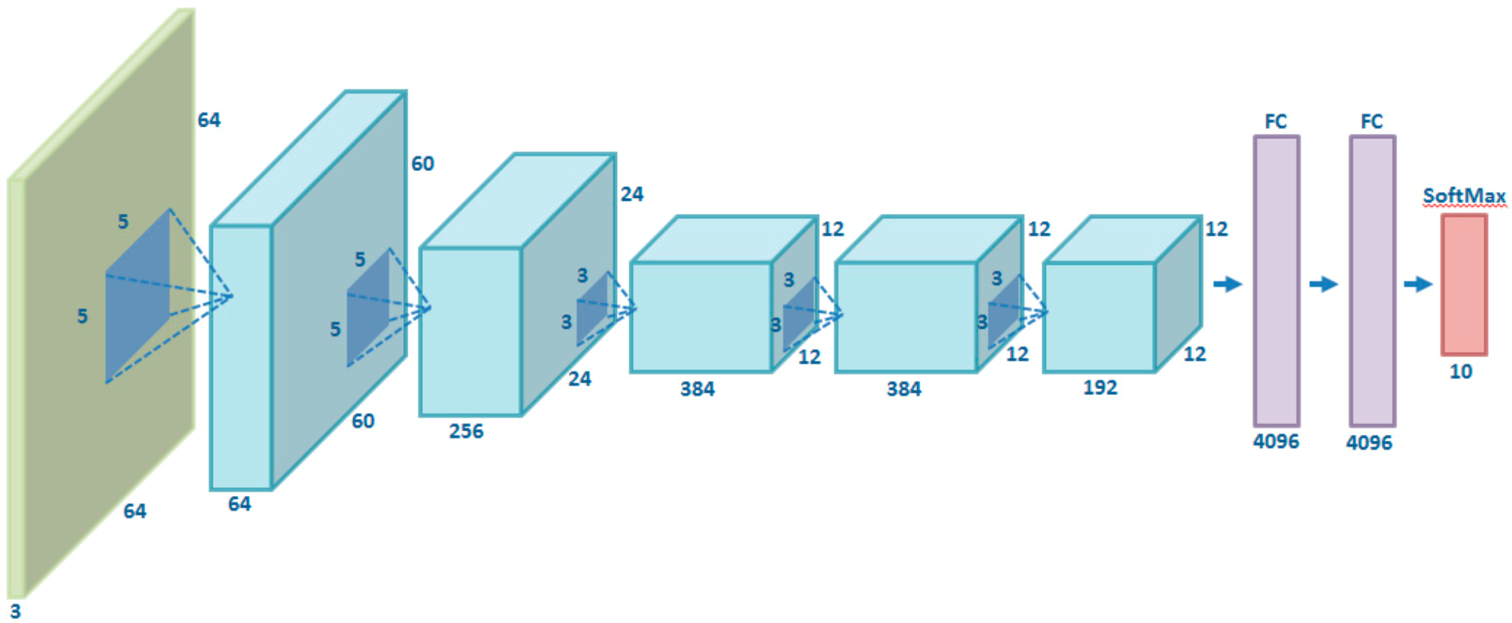
Figure 2.
Accuracy results of the AlexNet network using validation images.

Figure 3.
Reduction of associated cost during training of the AlexNet network.
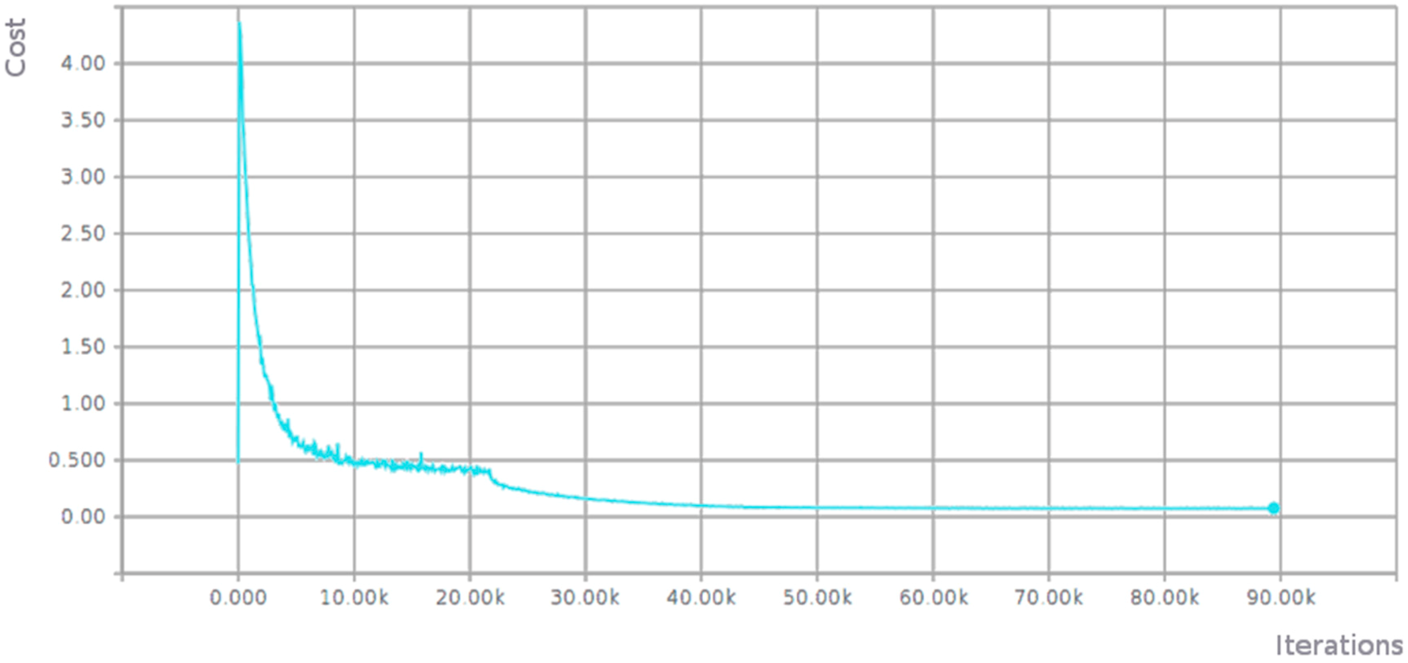
Figure 4.
(a) Visualization of the first layer at the beginning of the training; and (b) visualization of the first layer at the end of the training.
Figure 4.
(a) Visualization of the first layer at the beginning of the training; and (b) visualization of the first layer at the end of the training.
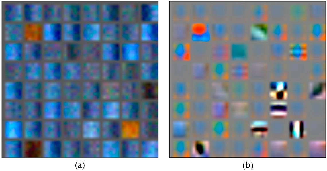
Figure 5.
Normal Convolutional Neural Network (left); and shortcut connections of ResNet architecture (right) [15].
Figure 5.
Normal Convolutional Neural Network (left); and shortcut connections of ResNet architecture (right) [15].

Figure 6.
Accuracy results of ResNet network.
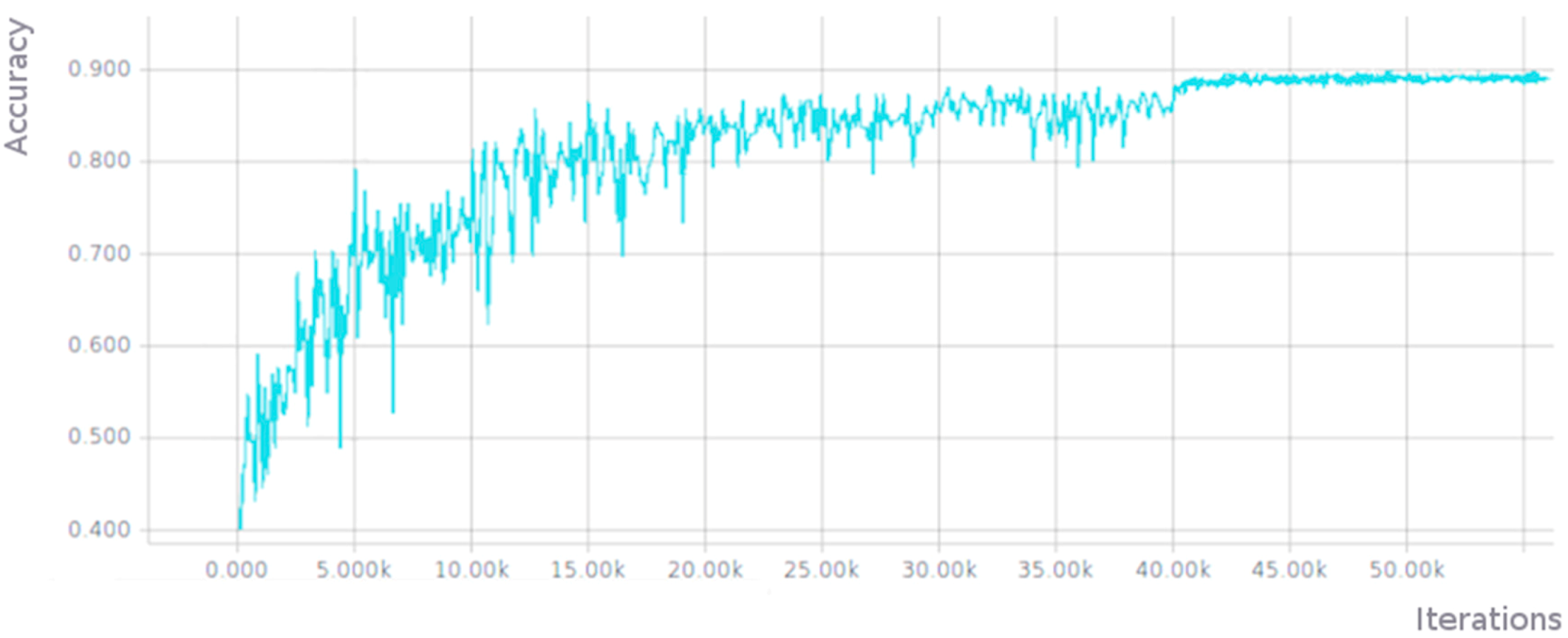
Figure 7.
Associated cost during training.
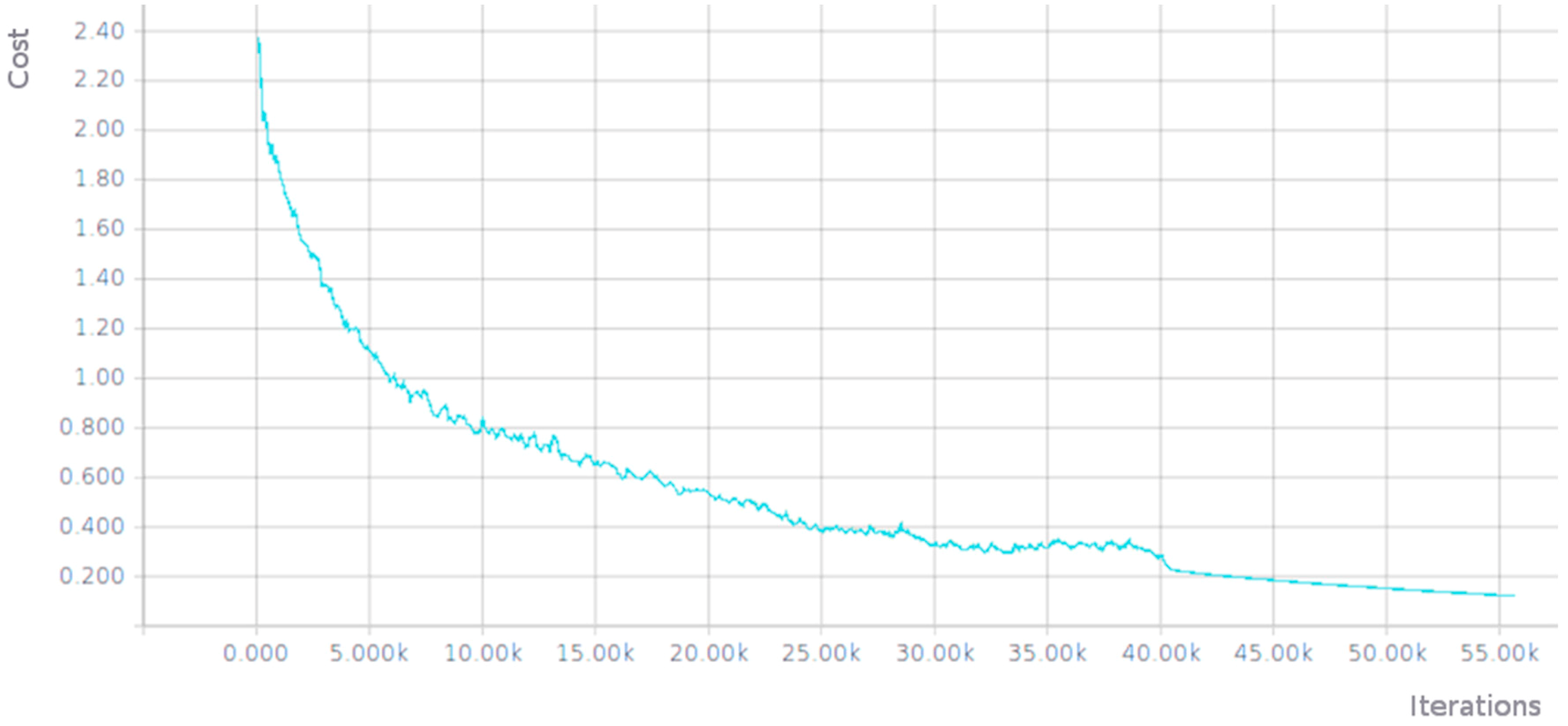
Figure 8.
Comparison of the training times of the cases considered.

Figure 9.
Comparison of the epochs needed in each case to reach convergence.
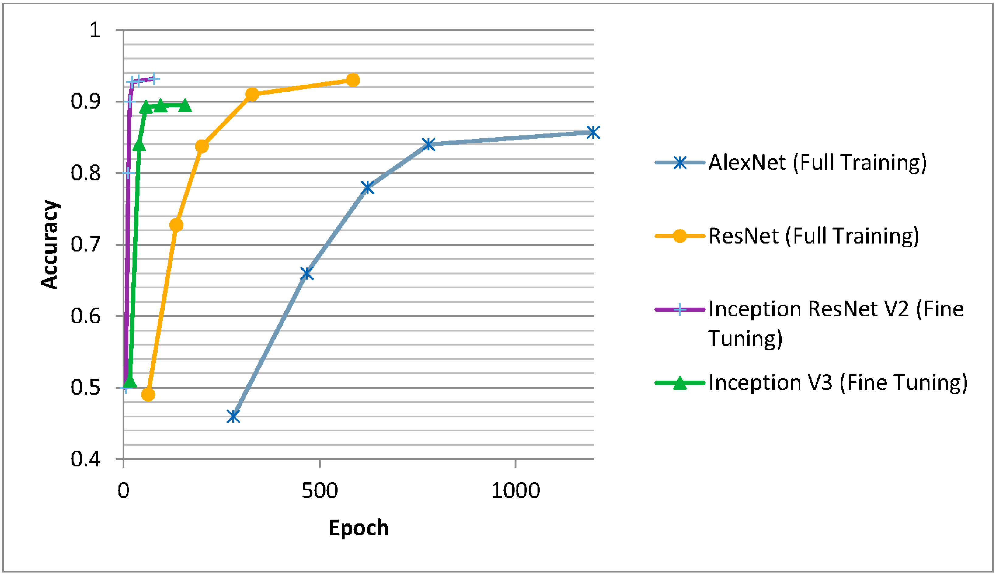

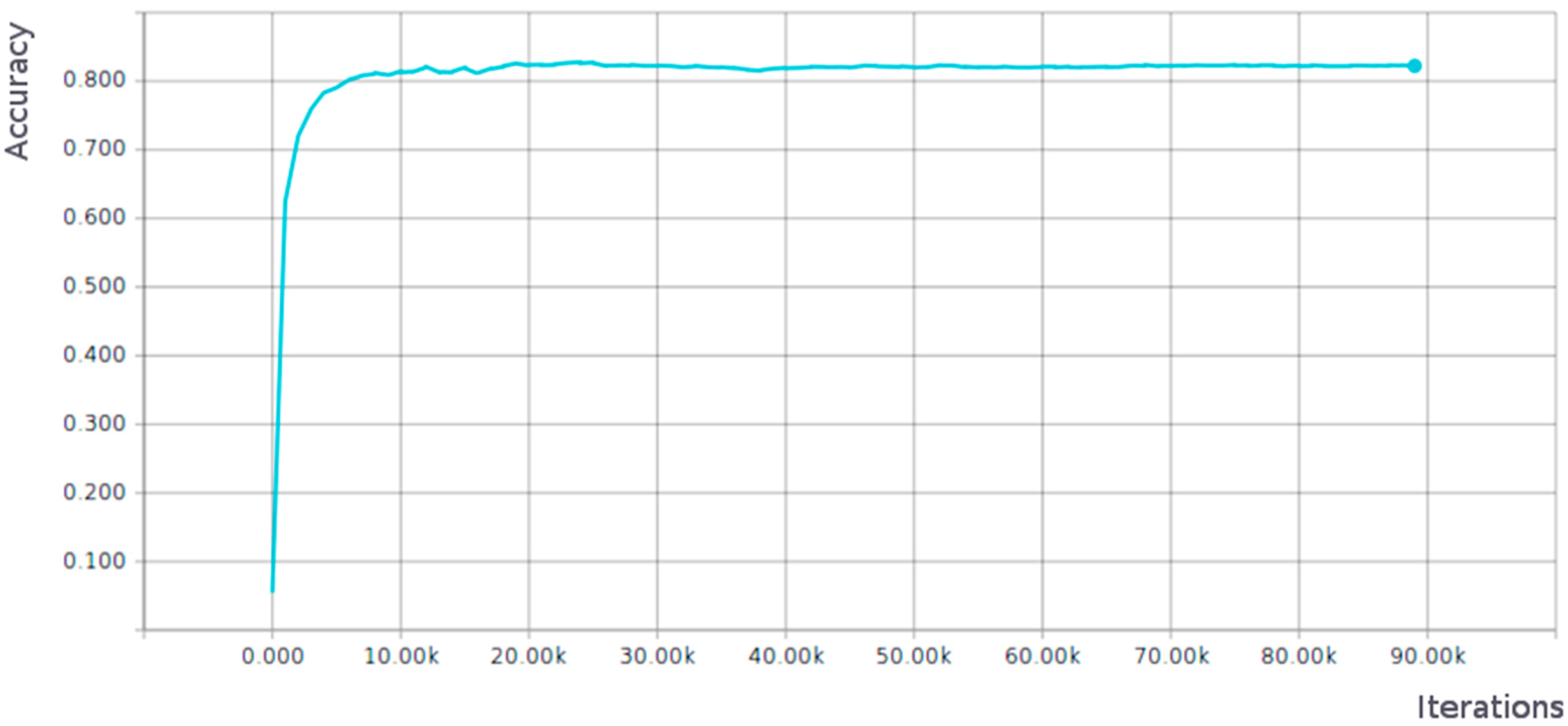
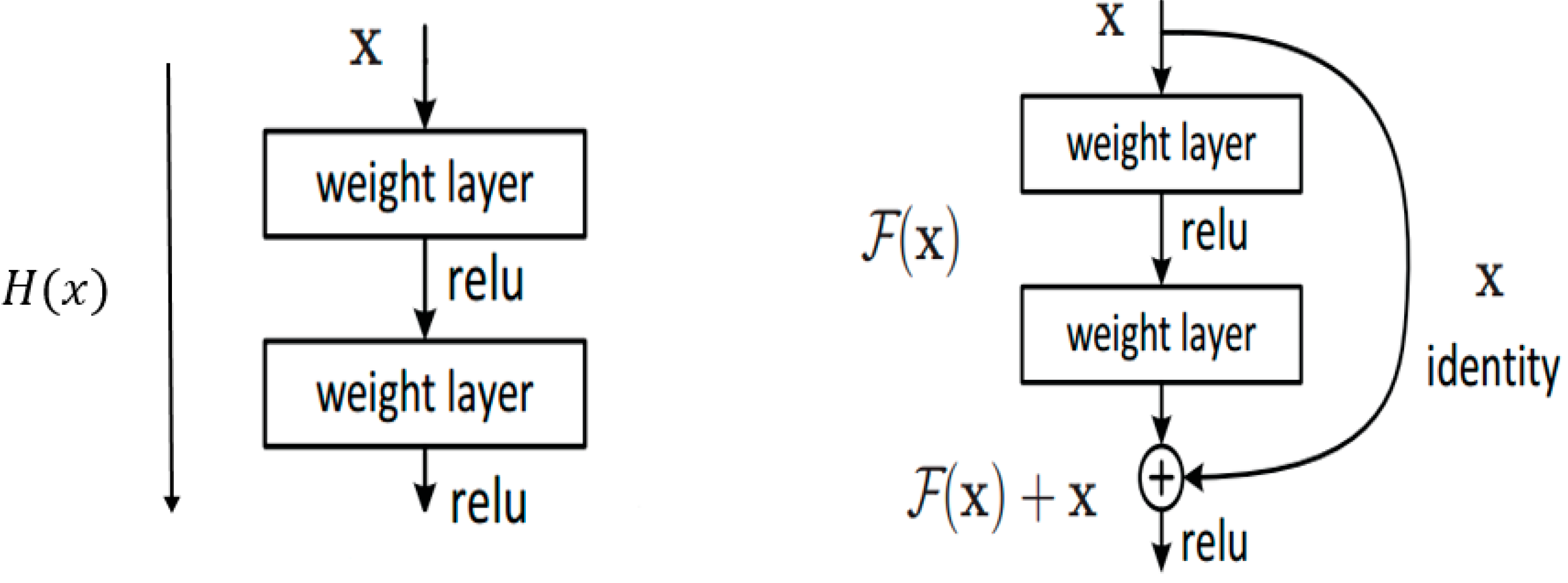
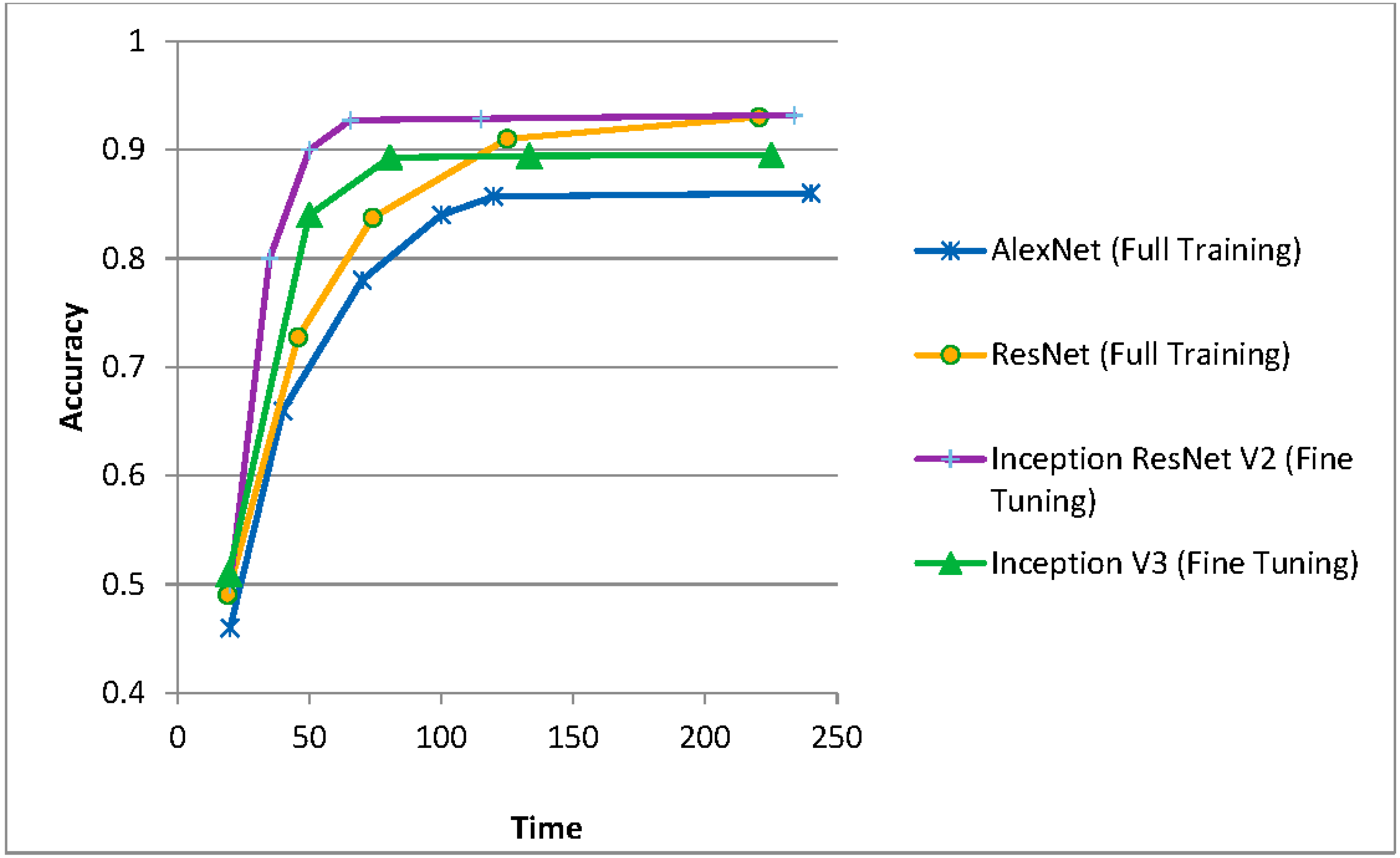
Table 1.
Dataset samples of Cultural Heritage images used.
| Category | Examples |
|---|---|
| Altar (829 images) |  |
| Apse (514 images) |  |
| Bell tower (1059 images) |  |
| Column (1919 images) |  |
| Dome (inner) (616 images) |  |
| Dome (outer) (1177 images) |  |
| Flying buttress (407 images) |  |
| Gargoyle (and Chimera) (1571 images) |  |
| Stained glass (1033 images) |  |
| Vault (1110 images) |  |
Table 2.
Hyperparameters used in the implemented AlexNet network.
| Momentum | Initial Learning Rate | Learning Rate Decay Factor | Moving Average Decay | Number of Epochs Per Decay | Weight Decay | Batch Size |
|---|---|---|---|---|---|---|
| 0.9 | 0.1 | 0.1 | 0.9999 | 350 | 0.0005 | 128 |
Table 3.
Hyperparameters used in the fine-tuning of an Inception V3 network.
| Momentum | Initial Learning Rate | Decay | Number of Epochs Per Decay | Weight Decay Rate | End Learning Rate | Batch Size |
|---|---|---|---|---|---|---|
| 0.9 | 0.01 | 0.94 | 2 | 0.00004 | 0.0001 | 32 |
Table 4.
Hyperparameters used in training the ResNet network.
| Momentum | Initial Learning Rate | Learning Rate Decay Factor | Number of Epochs Per Decay | Weight Decay Rate | End Learning Rate | Batch Size |
|---|---|---|---|---|---|---|
| 0.9 | 0.1 | 1/10 every 15,000 iter | 2 | 0.0002 | 0.0001 | 128 |
Table 5.
Hyperparameters used in the fine tuning of Inception-Resnet-v2 network.
| Momentum | Initial Learning Rate | Decay | Number of Epochs Per Decay | Weight Decay Rate | End Learning Rate | Batch Size |
|---|---|---|---|---|---|---|
| 0.9 | 0.01 | 0.94. | 2 | 0.00004 | 0.0001 | 32 |
Table 6.
Comparison of the accuracy results obtained in the different tests performed.
| Algorithm | Image Size | Accuracy | Epoch |
|---|---|---|---|
| AlexNet (Full Training) | 32 × 32 | 0.823 | 1400 |
| AlexNet (Full Training) | 64 × 64 | 0.857 | 1198 |
| ResNet (Full Training) | 32 × 32 | 0.896 | 949 |
| ResNet (Full Training) | 64 × 64 | 0.93 | 585 |
| Inception V3 (Fine Tuning) | 64 × 64 | 0.8943 | 93 |
| Inception V3 (Fine Tuning) | 128 × 128 | 0.9155 | 88 |
| Inception-ResNet-v2 (Fine Tuning) | 64 × 64 | 0.9103 | 82 |
| Inception-ResNet-v2 (Fine Tuning) | 128 × 128 | 0.9319 | 77 |
Table 7.
Confusion matrix obtained using a ResNet network (full-training) and the validation dataset (the rows correspond to the actual values and the columns to the predicted values).
Table 7.
Confusion matrix obtained using a ResNet network (full-training) and the validation dataset (the rows correspond to the actual values and the columns to the predicted values).
| Category | Altar | Apse | Bell Tower | Column | Dome (Inner) | Dome (Outer) | Flying Buttress | Gargoyle | Stained Glass | Vault | |
|---|---|---|---|---|---|---|---|---|---|---|---|
| Altar | 0.935 | 0.000 | 0.014 | 0.005 | 0.000 | 0.000 | 0.000 | 0.006 | 0.000 | 0.030 |  |
| Apse | 0.000 | 0.906 | 0.036 | 0.005 | 0.000 | 0.009 | 0.045 | 0.003 | 0.000 | 0.000 | |
| Bell tower | 0.000 | 0.000 | 0.886 | 0.003 | 0.000 | 0.013 | 0.000 | 0.036 | 0.000 | 0.000 | |
| Column | 0.028 | 0.000 | 0.014 | 0.965 | 0.000 | 0.004 | 0.015 | 0.022 | 0.000 | 0.030 | |
| Dome (inner) | 0.000 | 0.000 | 0.000 | 0.000 | 0.992 | 0.009 | 0.000 | 0.006 | 0.000 | 0.013 | |
| Dome (outer) | 0.000 | 0.063 | 0.032 | 0.000 | 0.000 | 0.964 | 0.000 | 0.022 | 0.000 | 0.000 | |
| Flying buttress | 0.000 | 0.031 | 0.018 | 0.013 | 0.000 | 0.000 | 0.896 | 0.025 | 0.000 | 0.004 | |
| Gargoyle | 0.000 | 0.000 | 0.000 | 0.000 | 0.000 | 0.000 | 0.045 | 0.866 | 0.000 | 0.004 | |
| Stained glass | 0.000 | 0.000 | 0.000 | 0.000 | 0.000 | 0.000 | 0.000 | 0.003 | 0.995 | 0.009 | |
| Vault | 0.037 | 0.000 | 0.000 | 0.008 | 0.008 | 0.000 | 0.000 | 0.011 | 0.005 | 0.909 |
Table 8.
Different metrics of the results obtained in each class using a ResNet network (full-training) and the validation dataset.
Table 8.
Different metrics of the results obtained in each class using a ResNet network (full-training) and the validation dataset.
| Measure | Altar | Apse | Bell Tower | Column | Dome (Inner) | Dome (Outer) | Flying Buttress | Gargoyle | Stained Glass | Vault |
|---|---|---|---|---|---|---|---|---|---|---|
| Recall (Sensitivity) | 0.878 | 0.845 | 0.920 | 0.940 | 0.944 | 0.911 | 0.732 | 0.987 | 0.986 | 0.941 |
| Precision | 0.935 | 0.906 | 0.886 | 0.965 | 0.992 | 0.964 | 0.896 | 0.866 | 0.995 | 0.909 |
| Specificity | 0.996 | 0.995 | 0.986 | 0.992 | 0.999 | 0.995 | 0.996 | 0.972 | 0.999 | 0.988 |
| Balanced accuracy | 0.937 | 0.920 | 0.953 | 0.966 | 0.972 | 0.953 | 0.864 | 0.979 | 0.992 | 0.965 |
| F1 score | 0.906 | 0.874 | 0.903 | 0.953 | 0.967 | 0.937 | 0.805 | 0.923 | 0.990 | 0.925 |
Table 9.
Confusion matrix obtained using a ResNet network (full-training) and the test dataset (the rows correspond to the actual values and the columns to the predicted values).
Table 9.
Confusion matrix obtained using a ResNet network (full-training) and the test dataset (the rows correspond to the actual values and the columns to the predicted values).
| Category | Altar | Apse | Bell Tower | Column | Dome (Inner) | Dome (Outer) | Flying Buttress | Gargoyle | Stained Glass | Vault | |
|---|---|---|---|---|---|---|---|---|---|---|---|
| Altar | 0.824 | 0.000 | 0.006 | 0.015 | 0.000 | 0.000 | 0.014 | 0.000 | 0.007 | 0.019 |  |
| Apse | 0.013 | 0.707 | 0.018 | 0.000 | 0.000 | 0.015 | 0.014 | 0.004 | 0.000 | 0.000 | |
| Bell tower | 0.000 | 0.086 | 0.888 | 0.021 | 0.000 | 0.036 | 0.000 | 0.024 | 0.000 | 0.000 | |
| Column | 0.044 | 0.086 | 0.018 | 0.944 | 0.000 | 0.007 | 0.014 | 0.028 | 0.007 | 0.006 | |
| Dome (inner) | 0.013 | 0.000 | 0.000 | 0.000 | 0.952 | 0.000 | 0.000 | 0.012 | 0.000 | 0.025 | |
| Dome (outer) | 0.000 | 0.052 | 0.047 | 0.000 | 0.000 | 0.942 | 0.000 | 0.004 | 0.000 | 0.006 | |
| Flying buttress | 0.006 | 0.000 | 0.012 | 0.005 | 0.000 | 0.000 | 0.914 | 0.008 | 0.000 | 0.000 | |
| Gargoyle | 0.006 | 0.034 | 0.012 | 0.010 | 0.000 | 0.000 | 0.043 | 0.920 | 0.000 | 0.000 | |
| Stained glass | 0.019 | 0.017 | 0.000 | 0.005 | 0.048 | 0.000 | 0.000 | 0.000 | 0.986 | 0.012 | |
| Vault | 0.075 | 0.017 | 0.000 | 0.000 | 0.000 | 0.000 | 0.000 | 0.000 | 0.000 | 0.932 |
Table 10.
Different metrics of the results obtained in each class using a ResNet network (full-training) and the test dataset.
Table 10.
Different metrics of the results obtained in each class using a ResNet network (full-training) and the test dataset.
| Measure | Altar | Apse | Bell Tower | Column | Dome (Inner) | Dome (Outer) | Flying Buttress | Gargoyle | Stained Glass | Vault |
|---|---|---|---|---|---|---|---|---|---|---|
| Recall (Sensitivity) | 0.936 | 0.820 | 0.882 | 0.876 | 0.870 | 0.908 | 0.914 | 0.958 | 0.933 | 0.920 |
| Precision | 0.824 | 0.707 | 0.888 | 0.944 | 0.952 | 0.942 | 0.914 | 0.920 | 0.986 | 0.932 |
| Specificity | 0.978 | 0.987 | 0.985 | 0.991 | 0.998 | 0.994 | 0.996 | 0.983 | 0.998 | 0.991 |
| Balanced accuracy | 0.957 | 0.904 | 0.933 | 0.933 | 0.934 | 0.951 | 0.955 | 0.971 | 0.966 | 0.956 |
| F1 score | 0.876 | 0.759 | 0.885 | 0.909 | 0.909 | 0.925 | 0.914 | 0.939 | 0.959 | 0.926 |
Table 11.
Examples of best predictions using the ResNet network.
 |  |  |  |  |
| Bell tower: 78.22% | Bell tower: 76.94% | Gargoyle: 57.11% | Dome (inner): 70.72% | Apse: 63.61% |
| Dome (outer): 19.39% | Dome (outer): 21.99% | Column: 33.95% | Vault: 27.02% | Column: 36.15% |
| Apse: 2.36% | Gargoyle: 0.71% | Flying buttress: 6.83% | Stained glass: 2.24% | Bell tower: 0.21% |
Table 12.
Examples of images incorrectly classified by the convolutional neural networks used.
| Correct Category | Images Incorrectly Classified (and the Corresponding Wrong Categories) | |||
|---|---|---|---|---|
| Altar |  Column |  Stained glass |  Vault | |
| Apse |  Dome (outer) |  Flying buttress |  Altar |  Bell tower |
| Bell tower |  Gargoyle |  Column |  Apse |  Dome(outer) |
| Column |  Altar |  Flying buttress |  Gargoyle |  Stained glass |
| Dome (inner) |  Vault |  Altar | ||
| Dome (outer) |  Bell tower |  Apse | ||
| Flying buttress |  Bell tower |  Gargoyle |  Altar | |
| Gargoyle |  Flying buttress |  Column |  Bell tower | |
| Stained glass |  Altar |  Column | ||
| Vault |  Altar |  Apse | ||
Table 13.
Comparison table of some methods using the dataset of architectural styles (25 categories).
Table 13.
Comparison table of some methods using the dataset of architectural styles (25 categories).
| Algorithm | Image Size | Accuracy | Epoch |
|---|---|---|---|
| MLLR + SP | Different sizes (typically 800 × 600) | 0.4621 | |
| DPM (Deformable part-based model)-LSVM | Different sizes (typically 800 × 600) | 0.3769 | |
| OB (Object bank)-Part | Different sizes (typically 800 × 600) | 0.4541 | |
| SP (Spatial pyramid) | Different sizes (typically 800 × 600) | 0.4452 | |
| Inception V3 (Fine Tuning) | 64 × 64 | 0.5567 | 65 |
| Inception-ResNet-v2 (Fine Tuning) | 64 × 64 | 0.5433 | 116 |
© 2017 by the authors. Licensee MDPI, Basel, Switzerland. This article is an open access article distributed under the terms and conditions of the Creative Commons Attribution (CC BY) license (http://creativecommons.org/licenses/by/4.0/).
Share and Cite
MDPI and ACS Style
Llamas, J.; M. Lerones, P.; Medina, R.; Zalama, E.; Gómez-García-Bermejo, J. Classification of Architectural Heritage Images Using Deep Learning Techniques. Appl. Sci. 2017, 7, 992. https://doi.org/10.3390/app7100992
AMA Style
Llamas J, M. Lerones P, Medina R, Zalama E, Gómez-García-Bermejo J. Classification of Architectural Heritage Images Using Deep Learning Techniques. Applied Sciences. 2017; 7(10):992. https://doi.org/10.3390/app7100992
Chicago/Turabian StyleLlamas, Jose, Pedro M. Lerones, Roberto Medina, Eduardo Zalama, and Jaime Gómez-García-Bermejo. 2017. "Classification of Architectural Heritage Images Using Deep Learning Techniques" Applied Sciences 7, no. 10: 992. https://doi.org/10.3390/app7100992
Note that from the first issue of 2016, this journal uses article numbers instead of page numbers. See further details here.