The Deep Belief and Self-Organizing Neural Network as a Semi-Supervised Classification Method for Hyperspectral Data

1
School of Economics and Management, Beihang University, Beijing 100191, China
2
Fundamental Science on Ergonomics and Environment Control Laboratory, School of Aeronautics Science and Engineering, Beihang University, Beijing 100191, China
*
Author to whom correspondence should be addressed.
Appl. Sci. 2017, 7(12), 1212; https://doi.org/10.3390/app7121212
Submission received: 12 September 2017
/
Accepted: 8 November 2017
/
Published: 24 November 2017
Abstract
:Hyperspectral data is not linearly separable, and it has a high characteristic dimension. This paper proposes a new algorithm that combines a deep belief network based on the Boltzmann machine with a self-organizing neural network. The primary features of the hyperspectral image are extracted with a deep belief network. The weights of the network are fine-tuned using the labeled sample. Feature vectors extracted by the deep belief network are classified by a self-organizing neural network. The method reduces the spectral dimension of the data while preserving the large amount of original information in the data. The method overcomes the long training time required when using self-organizing neural networks for clustering, as well as the training difficulties of Deep Belief Networks (DBN) when the labeled sample size is small, thereby improving the accuracy and robustness of the semi-supervised classification. Simulation results show that the structure of the network can achieve higher classification accuracy when the labeled sample is deficient.

1. Introduction
Spectral imaging technology combines spatial imaging with spectral analysis. This technology has extensive military and civilian applications [1,2,3,4,5]. Spectral imaging, especially hyperspectral imaging, has advantages in being able to distinguish features (its spectral and spatial distinguishing ability), data size, and wavebands. However, with a smaller sample size for data analysis [6,7], the curse of dimensionality, and, concurrently, linear classification faults, this technology may well show its deficiencies [8,9]. At present, there are several more mature classification methods that can be applied to hyperspectral data, including support vector machines (SVMs) and spectral angle mapping (SAM) [10,11,12,13,14,15]. With SVMs [16,17], storage and computing are expensive when the number of training samples is large. Solving multiple classification problems can be difficult [18,19]. One may need to take advantage of the known categories of training samples. Spectral angle mapping (SAM) relies on a standard expert database [20,21]. This method has more applications in multispectral imaging when combined with other algorithms. In addition, the dimensionality of hyperspectral data is too high and needs to be reduced. Ordinary dimensional reduction methods, such as principal component analysis (PCA) [17,22], band selection [23], MNF conversion [24], and other methods, come with the cost of a loss of information. We can effectively reduce the dimensionality of a hyperspectral data block using the index of the Gauss optimization method, but this method primarily extracts the characteristics of the absorption band while ignoring other spectral information. A Deep Belief Network (DBN) is composed of Restricted Boltzmann Machines (RBM) [25]. When the global energy function reaches its minimum, the DBN achieves its convergence condition. Also, it can learn, without supervision and maximum data, to achieve the goal of reducing the dimensionality of the data under the condition that much of the original information in the data is retained [19,26]. The classification of hyperspectral data has the problem of a linearly inseparable and high-sample dimension, and the classification accuracy is low when the sample label data is less. This paper uses a semi-supervised Self-Organizing feature Map (SOM) neural network, which can attain higher classification accuracy than other algorithms in the case of a small amount of labeled samples. Furthermore, the dimensionality reduction using the deep belief neural (DBN) network can well map the original spectral data. This method can solve the linearly inseparable problem of hyperspectral data in a certain extent. In addition, the method of dimensionality reduction using the DBN network solves the problem of the long training time of the SOM network in large data cases. So, this method can be used to realize the semi-supervised classification of original data information by using dimension-effective reduction, overcoming the difficulty of the long training time of clustering using the SOM network and fewer sample labels of the deep-learning algorithm training. This method has been successfully applied to the classification of hyperspectral data [27,28]. The problems of traditionally self-organizing [29] neural networks having a long training time for clustering, as well as the difficulty of training when using deep learning when labeled samples are insufficient, are solved [29,30]. Classification accuracy and robustness are improved at the same time.
2. Algorithm Introduction
2.1. Algorithm Procedure
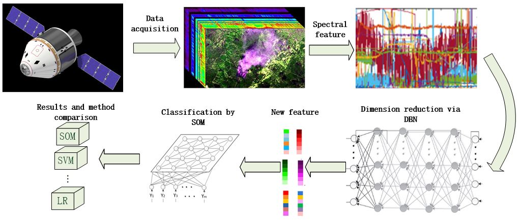
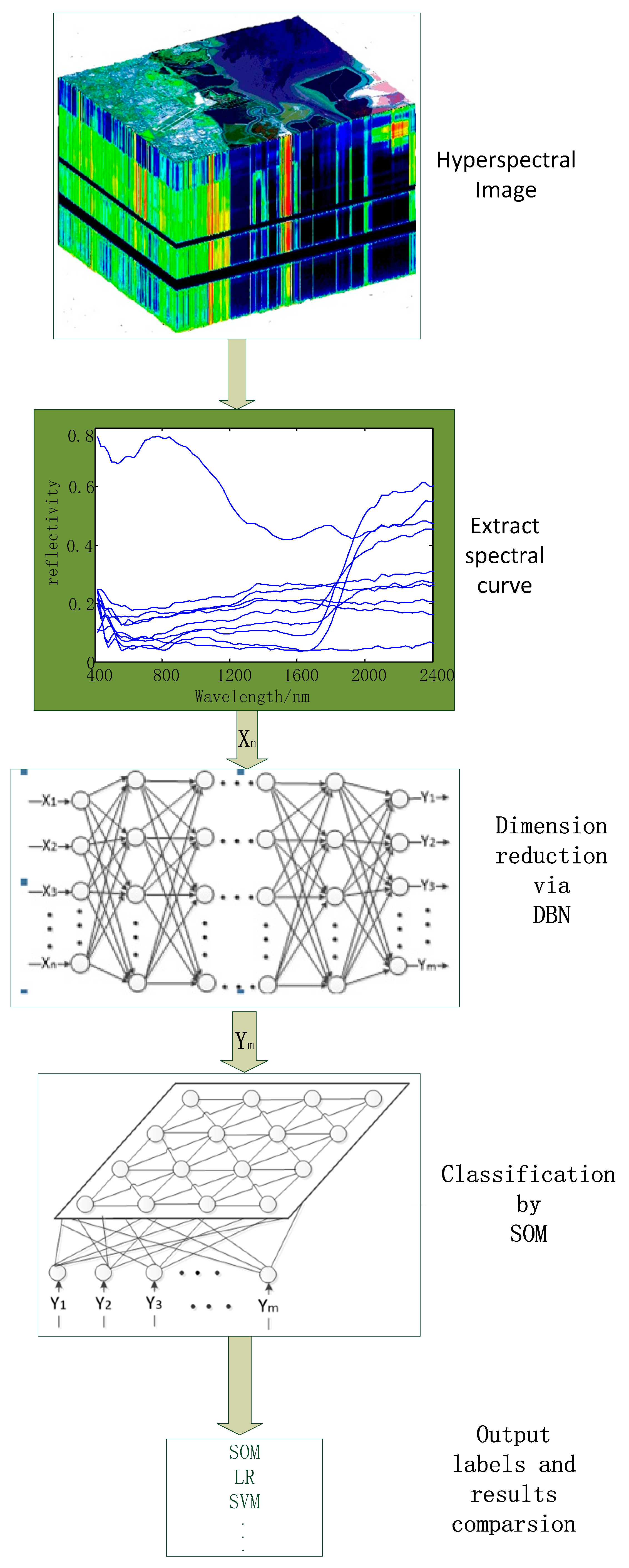
The algorithm flow chart is shown in Figure 1. First, all of the spectral curves from hyperspectral image are extracted. To perform calculations conveniently, the intensity of spectral reflection is transformed into reflectivity. Second, all of the spectral curves are input into the DBN, and their dimensions are reduced to yield the curves . The dimension of dimensionally reduced data must be consistent with the total number of categories. Third, fine tuning with several labeled samples is performed. Finally, the input characteristic matrix that is generated from the original data is input into the SOM, which outputs the classification results.
The entire network achieves its function of classification by mapping the original data continuously. However, before classification, the weights of each network need to be determined through training. The training process used in this paper is briefly introduced in the next section.
2.2. Network Training
The spectral dimensions of hyperspectral data are high, and the spectra contain rich information. However, if the spectra are used directly for classification, not only will the training time be long, but it will also make the classification accuracy lower due to the high spectral dimensionality of the sample. This phenomenon is the so-called curse of dimensionality. In this paper, a DBN is used to reduce the dimension of spectral data with no labels. During the training process, the weights of the network are fine-tuned with a few labeled samples to learn the inherent characteristics of the data and increase the separability of the characteristic data. Finally, the network’s weights and offsets are determined by training an SOM with the data after its dimensions have been reduced.
Based on the feature that the DBN only learns using the data without labels, two types of data sets are present in this flow chart, namely, training samples without labels and labeled samples for fine tuning [31]. The training samples are used to train the DBN and the SOM; the fine tuning samples are a subset of training samples that have been manually labeled [26,27,32]. Fine tuning is used to learn the category data which is already known from the training process. This approach can improve the classification accuracy, which will be verified in the following section. The flow chart of network training is shown in Figure 2.
2.2.1. Deep Belief Network
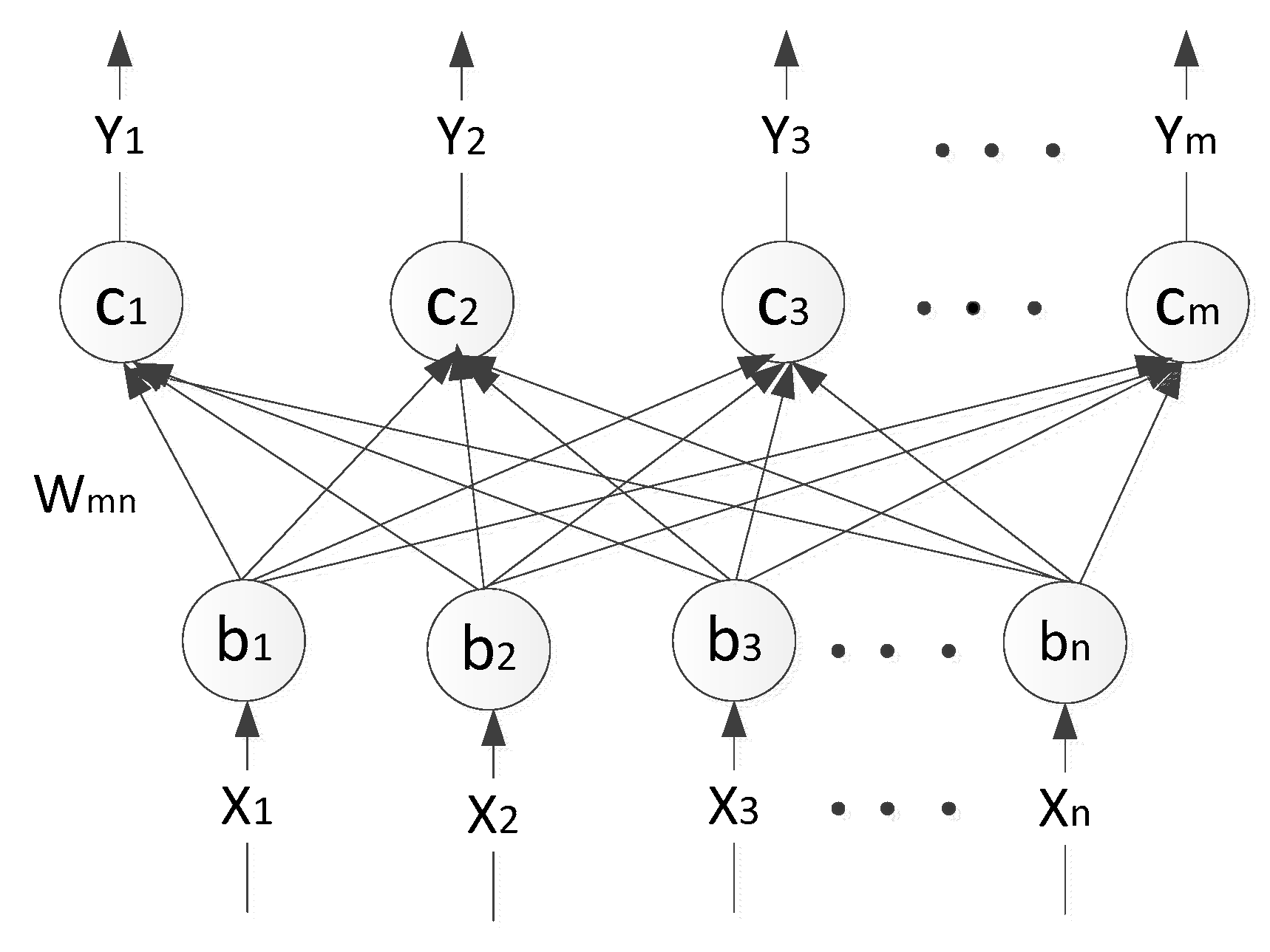
The function of the DBN is to initialize the weights of the deep learning network in order to solve gradient diffusion problem caused by the use of the gradient descent method used to correct the weights [33,34]. This network is comprised of a few Restricted Boltzmann Machine Networks [35,36]. The topological graph of Restricted Boltzmann Machine Network is shown in Figure 3.
The Restricted Boltzmann Machine network consists of two layers, namely, the visible layer and the hidden layer. The neurons between the two layers are fully connected, while the neurons in the peer layer are mutually independent. Both of the layers meet the Boltzmann distribution. Using conditional probability, the two layers can be refactored. When the difference between the hidden reconstruction vector and the input sample set is less than the minimum value that is already set, the training will be finished. The three parameters determined by training are the net weight Wmn the offset , and , where
The energy equation is
where
The joint probability density is
The weight updating formula is as follows (for learning rate, k for the number of cycles):
where
The Sigmoid function is defined as follows:
Deep belief net training can be regarded as successively training several Boltzman machine networks limited to two layers, using unsupervised learning from the bottom to the top layer. The intent is to match the features of the data as much as possible. Moreover, in order to improve the accuracy, robustness, and stability of the classification results and to enhance the divisibility of the data, computations in this paper also use samples with categories that are known in order to train the network. In other words, this approach supervises fine-tuning of the network from the top to the bottom using the gradient descent method.
The specific training program Algorithm 1 flowchart is as follows, in which is for training samples, is for fine-tuning samples, and is for fine-tuning sample tags:
| Algorithm 1 |
| 1. init for ; |
| 2. Input ; |
| 3. For ; |
| 4. Train |
| 5. |
| 6. End |
| 7. If Fine tune training |
| 8. Input using Gradient descent method |
| 9. Endif |
| 10. Output for ; |
2.2.2. Training of Self-Organizing, Competitive Neural Network
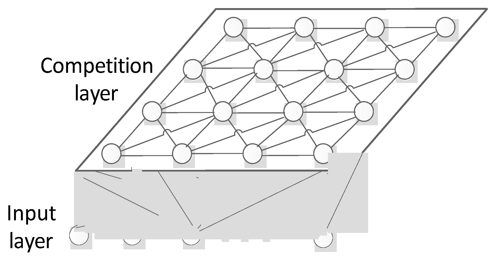
A self-organizing, competitive neural network can be used to learn the data without labels. This network can also squeeze the high-dimensional data into lower-dimensional space [38,39] in cases when the topological structure is unchanged. In consideration of the variety and structure characteristics of the hyperspectral data, the competition layer in this paper is selected as a two-dimensional surface. A topological graph is shown in Figure 4.
The input layer of the network takes as input in the eigenmatrix; it is extracted from the original data by the network. The weights update formula is shown in Formula (13),
where , ;
The superior domain update is
The learning rate is
3. Test Experiment
3.1. Data Sources
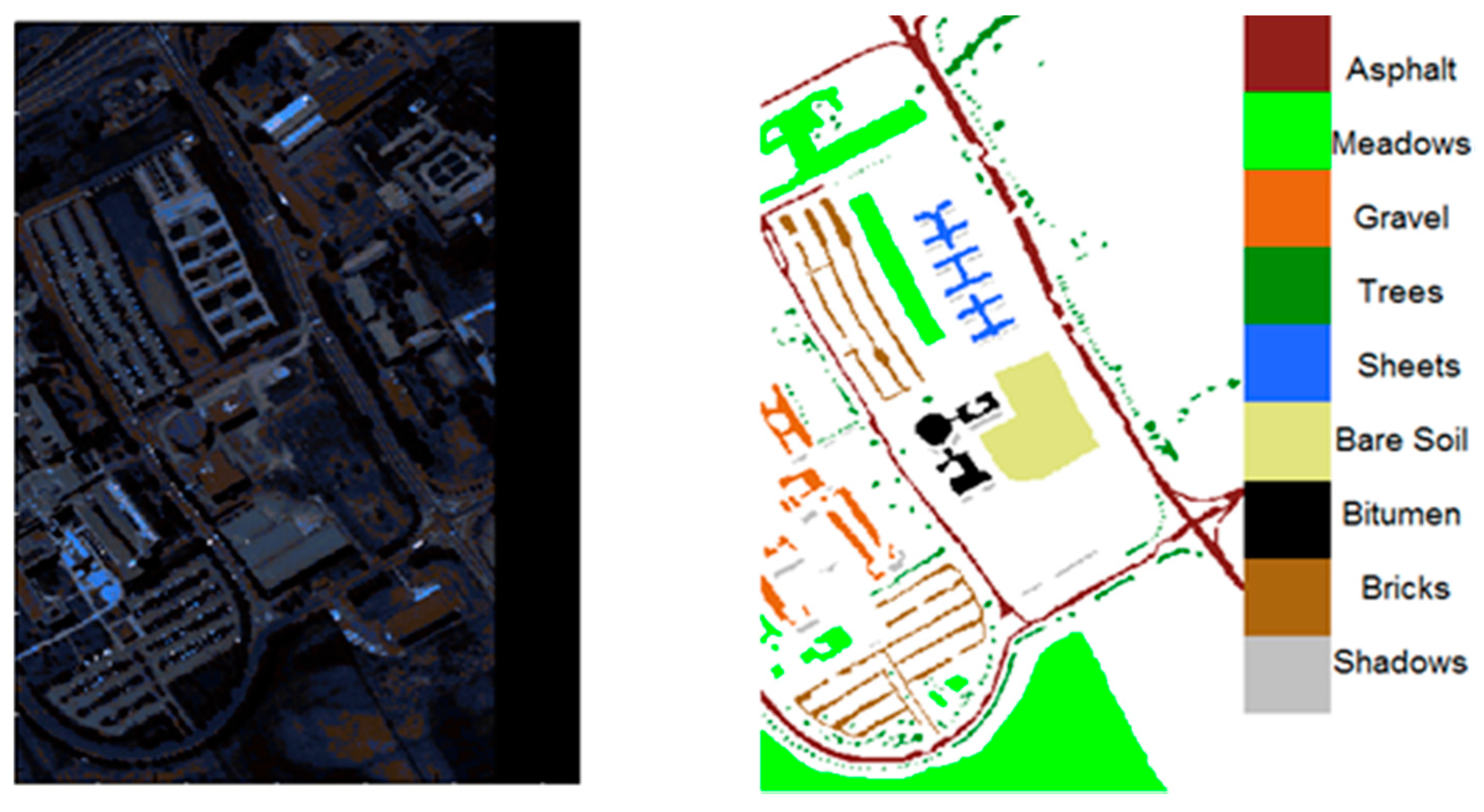
The hyperspectral data cube from the University of Pavia was acquired by the German aerial spectrometer ROSIS while it was flown through Pavia, a city in northern Italy. The classified data is shown in Figure 5. Data of the University of Pavia is comprised of 610 × 610 pixels, with a spectral resolution (number of wavelengths) of 103 and a ground resolution of approximately 1.3 m. Moreover, the data include 9 different types of objects. Black stripes in the image are where invalid data have been eliminated. In this paper, 6 types of data containing 31,116 samples are used.
3.2. Dimension Reduction of Deep Belief Net
A deep belief neural net converted the probability model into an energy model to capture the correlation between the training samples. In the case where a specific distribution is unknown, the lower energy, the lower the correlation will be. Therefore, characteristics of the data extracted without supervision can fit the original signal very well, effectively avoiding the curse of dimensionality and improving the classification accuracy.
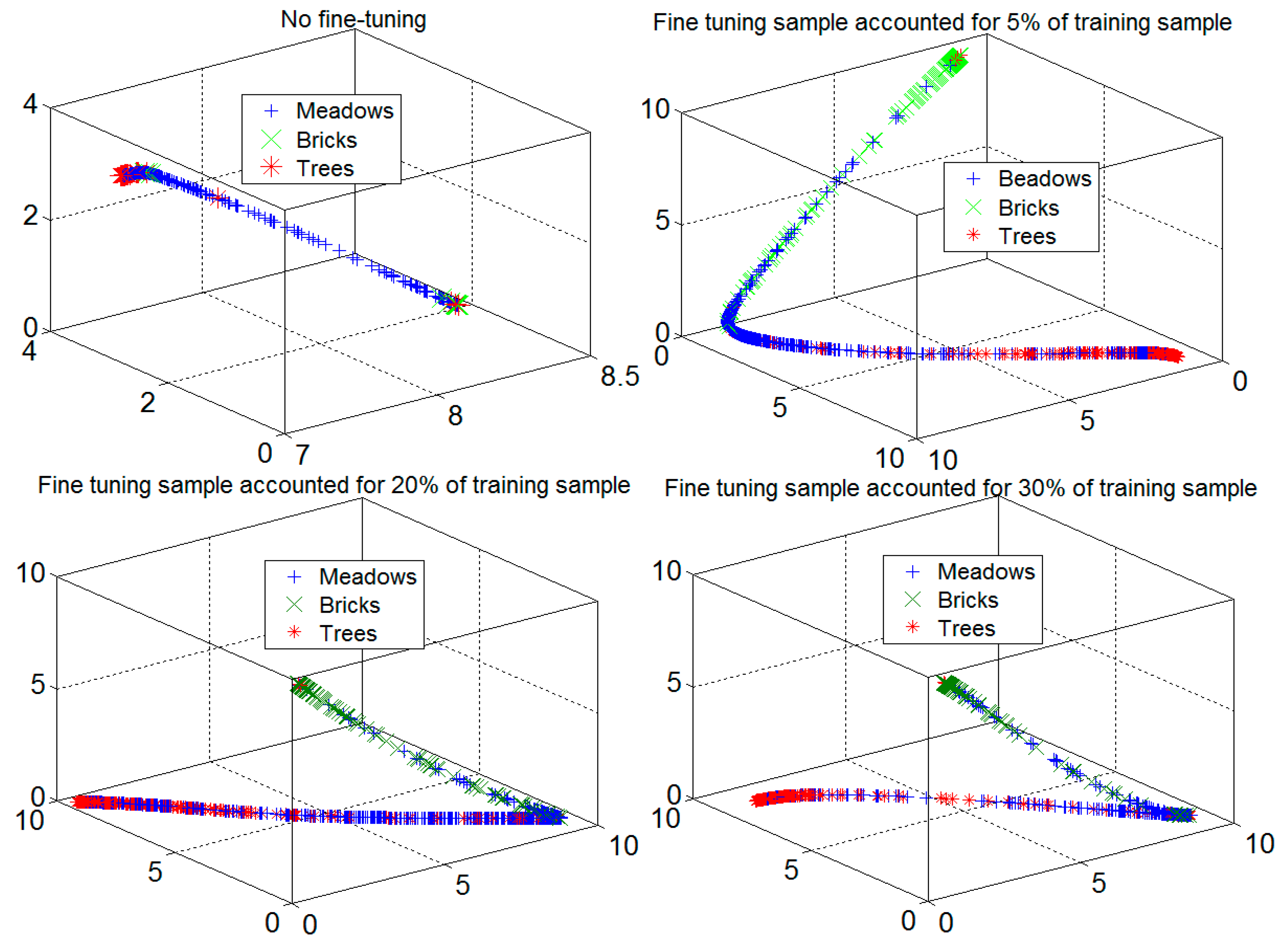
For ease of illustration, this article extracted three different categories of hyperspectral data from the image hypercube of the University of Pavia. By increasing the number of fine-tuning samples, characteristic profiles were determined for 5000 samples, as shown in Figure 6.
As seen from Figure 6, before fine-tuning, the data after dimensional reduction is inseparable in 3d space. After increasing the number of fine-tuning samples, the separability of characteristic data with dimensional reduction is more apparent, but not linear. The number of fine-tuning samples were 30% and 5% of the training samples; the separability of data is quite obvious, as shown in the figure.
3.3. Research of Label Sample Size and Classification Accuracy
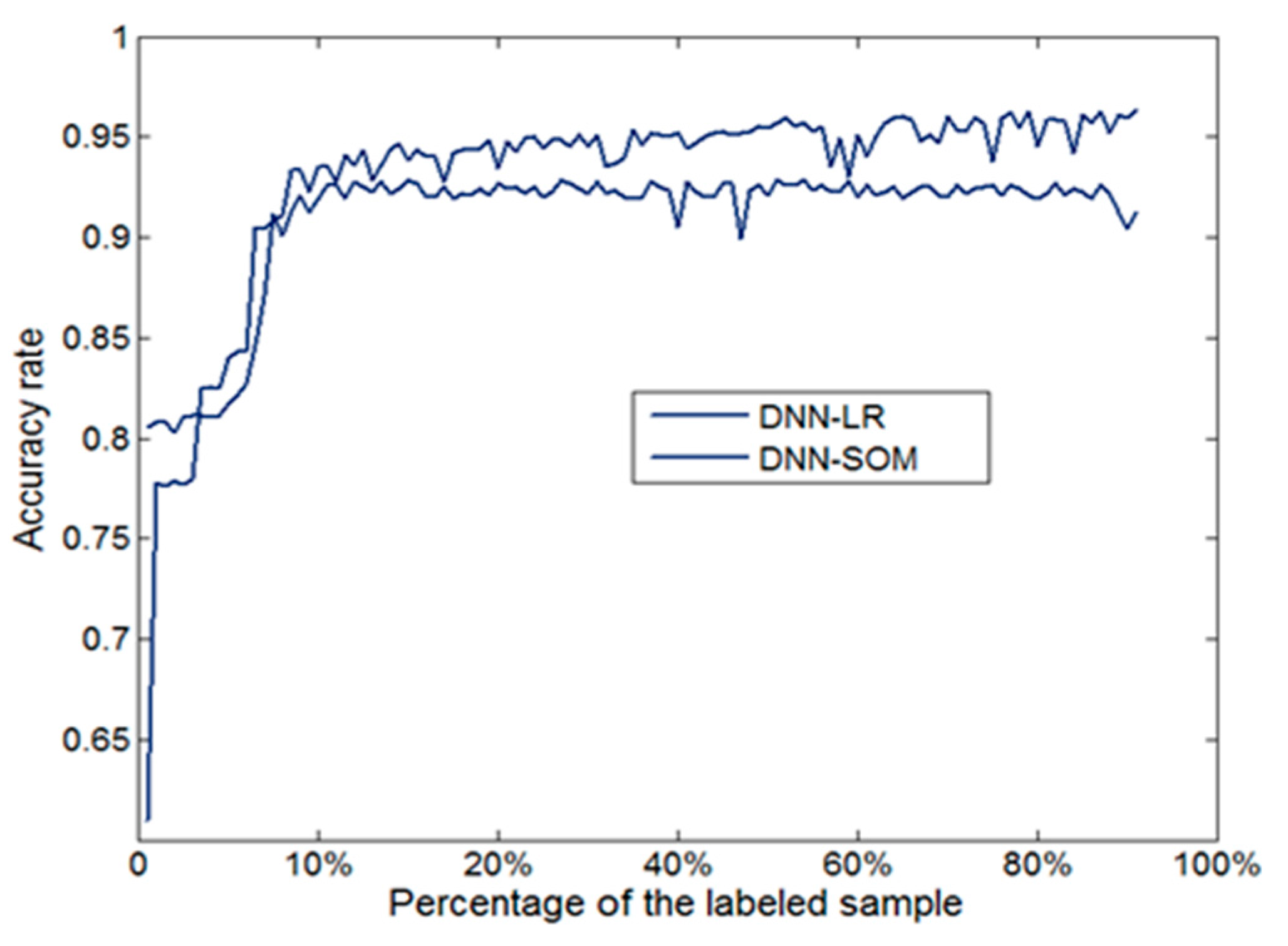
In the case of a sufficient number of sample labels, the deep belief net with dimensional reduction can achieve the desired classification accuracy using logistic regression. In this paper, a semi-supervised, self-organizing time network is used to solve the problem of the classification accuracy of a network that is low when the label sample size is small. For this reason, a simulation experiment was designed. In this experiment, the final layer of the deep belief net uses logistic regression and a self-organizing neural network. The result is shown in Figure 7.
Figure 7 illustrates that when the labeled sample size is less than 5% of the number of total training samples, classification accuracy using logistic regression is lower than when using a self-organizing neural network. When the labeled sample size is more than 10%, the average accuracy using logistic regression and a self-organizing neural network is, respectively, 5.35% and 92.82%. Therefore, we see that using a self-organizing neural network can guarantee classification accuracy in the case of a small labeled sample size.
3.4. Classification Results of Public Hyperspectral Databases
To test the usefulness of the method, three public hyperspectral databases were chosen for study. In all of the experiments, the deep belief network and a self-organizing network were applied. The color difference between the classification map and ground truth image is present, since the self-organized network is an unsupervised clustering method. The following are the experimental results.
As we can see from Figure 8, the scene was acquired by the ROSIS sensor during a flight over Pavia in northern Italy. The original data is composed of 115 spectral bands, ranging from 0.43 to 0.86 μm, each with a bandwidth of 4 nm. Noisy bands were previously discarded, leaving 102 channels in the image cube. The image of Pavia Center is a 1096 × 715 pixel image. Both of the image ground truths differentiate 9 classes each. For this data set, a total of 148,125 pixels were available for the study. As can be seen in Figure 8b, on the right is the ground truth, while in Figure 8a, on the left are the experimental results based on DBN and SOM. The edge of every class can be recognized easily. The algorithm has basically clustered related pixels into individual classes.
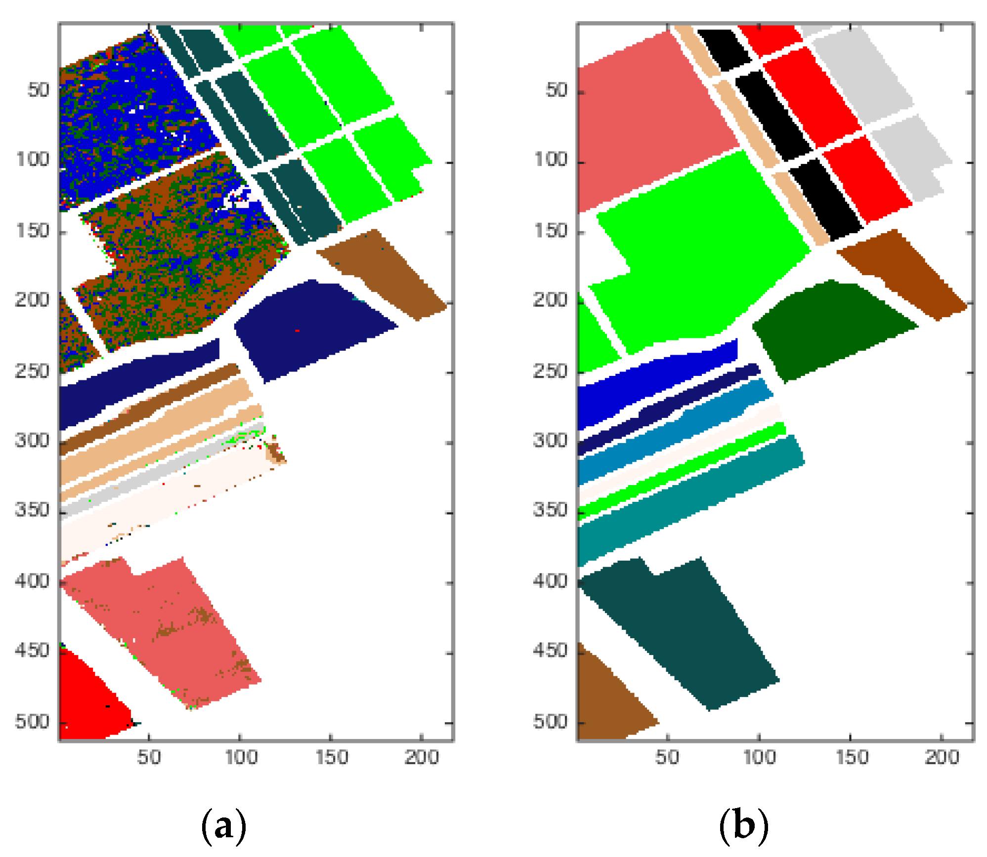
The scene shown in Figure 9 was also captured by the ROSIS sensor during a flight over Pavia in northern Italy. Noisy bands were also discarded, and the final number of spectral bands was 102 for the image of Pavia Center University. The image of Pavia Center University is comprised of 610 × 340 pixels. There were nine categories that needed to be classified. Figure 9a on the left is the result of this analysis, while Figure 9b on the right is the ground truth. Using DBN and SOM worked well visually on this hyperspectral image.
The scene in Figure 10 was collected by the 224-band AVIRIS sensor of the Salinas Valley, California and is characterized by a high spatial resolution (3.7-m pixels). The area covered is composed of 512 × 217 pixels. The Salinas ground truth contains 16 classes. We generated the ground truth image on the right and classified the hyperspectral image into 16 classes using the DBN and SOM. The result is displayed on the left in Figure 10a.
4. Comparative Experiments
4.1. Simulation
4.1.1. Simulation Data Source
A high-resolution spectral data cube of the University of Pavia was acquired using the German aerial photography spectroradiometer ROSIS. The image was taken in the northern Italian city of Pavia, as shown in Figure 5. The image is composed of 610 × 610 pixels, the number of spectral bands is 103, and the spatial resolution is approximately 1.3 m; the processed data contains nine different categories. The black region of the figure contained invalid data and is excluded. In this paper, 6 data classes were used, and 31,116 samples were taken.
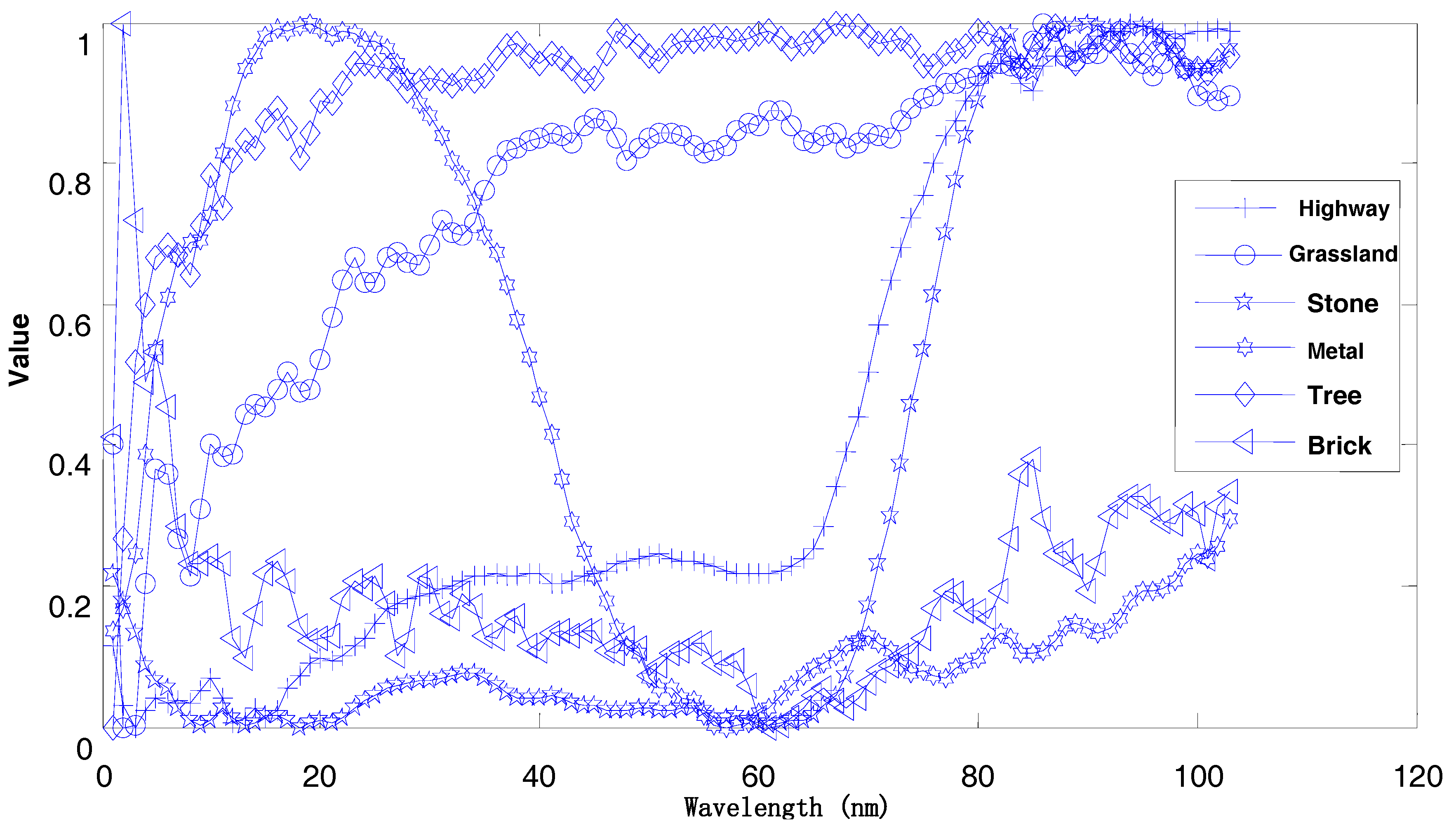
Figure 11 shows the corresponding spectral curves for the different categories of objects in the image. As can be observed from the diagram, the different objects have spectral absorption features; hence, the spectral curves are also different. The trained classification algorithm can identify the unknown object to which the spectral curves belong.
4.1.2. Depth Study of Deep Learning Network
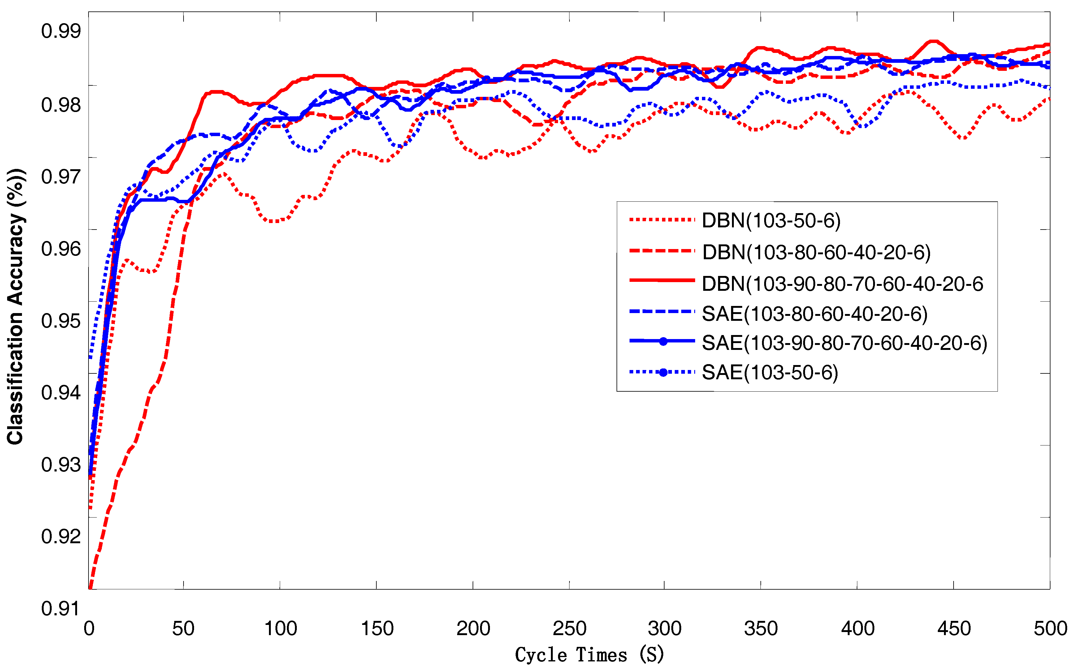
In theory, the more hidden layers there are, the more detailed the characterization of the data is, and the greater the ability to obtain more information about the data. However, the training time of the hidden layers will also increase, and the computer’s memory requirements will increase. To extract information from the University of Pavia hyperspectral data and not increase the training time and memory usage, a cyclic network structure was developed. The result is shown in Figure 7. The network structures shown are 103-50-6, 103-80-60-40-20-6, and 103-90-80-70-60-40-20.
As shown in Figure 12, when network training is stable and the network depth is 103-50-6, the classification accuracy is approximately 97%; the remaining two types of networks have a classification accuracy of approximately 98%. The deeper the network depth is, the more hidden the layers are, and the higher the corresponding increase in classification accuracy is. When depth is increased the network training time and memory usage increases accordingly. To ensure classification accuracy, save computer hardware resources, and save time, the depth of the learning network structure was chosen to be 40-80-60-103-20-6. In addition, the optimal network structure for different data sets is often different, and different network structures can achieve the same classification accuracy with an adjustment of the initial parameters. The optimal choice of network structure does not have theoretical support and can only be obtained by experiment.
4.1.3. Cycle Number Selection
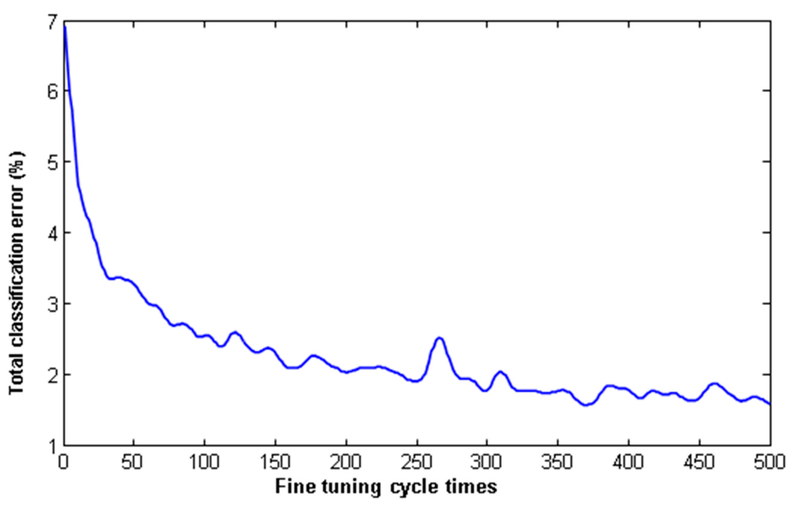
In theory, the more training repetitions that are used, the more detailed the study of data characteristics is, and the higher the classification accuracy is. There are two ways to select cycle times: a value can be set based on experience, or a minimum value for the total classification error can be set, and the program will select the number of training cycles. The optimal cycle times for different data sets or different network initial values are often different. Figure 13 shows the experimental results for the optimal cycle times based on the learning rate for the data set of the University of Pavia.
As seen in Figure 13, when the number of network training cycles is less than 350, the classification accuracy increases with the increase in the number of cycles. When the number of cycles is greater than 350, the classification accuracy increases with the number of cycles, but the rate of increase has obviously slowed. The greater the number of cycles, the greater the classification accuracy, but the training time increases correspondingly. Therefore, it is necessary to consider the two aspects of classification accuracy and training time when selecting the number of cycles.
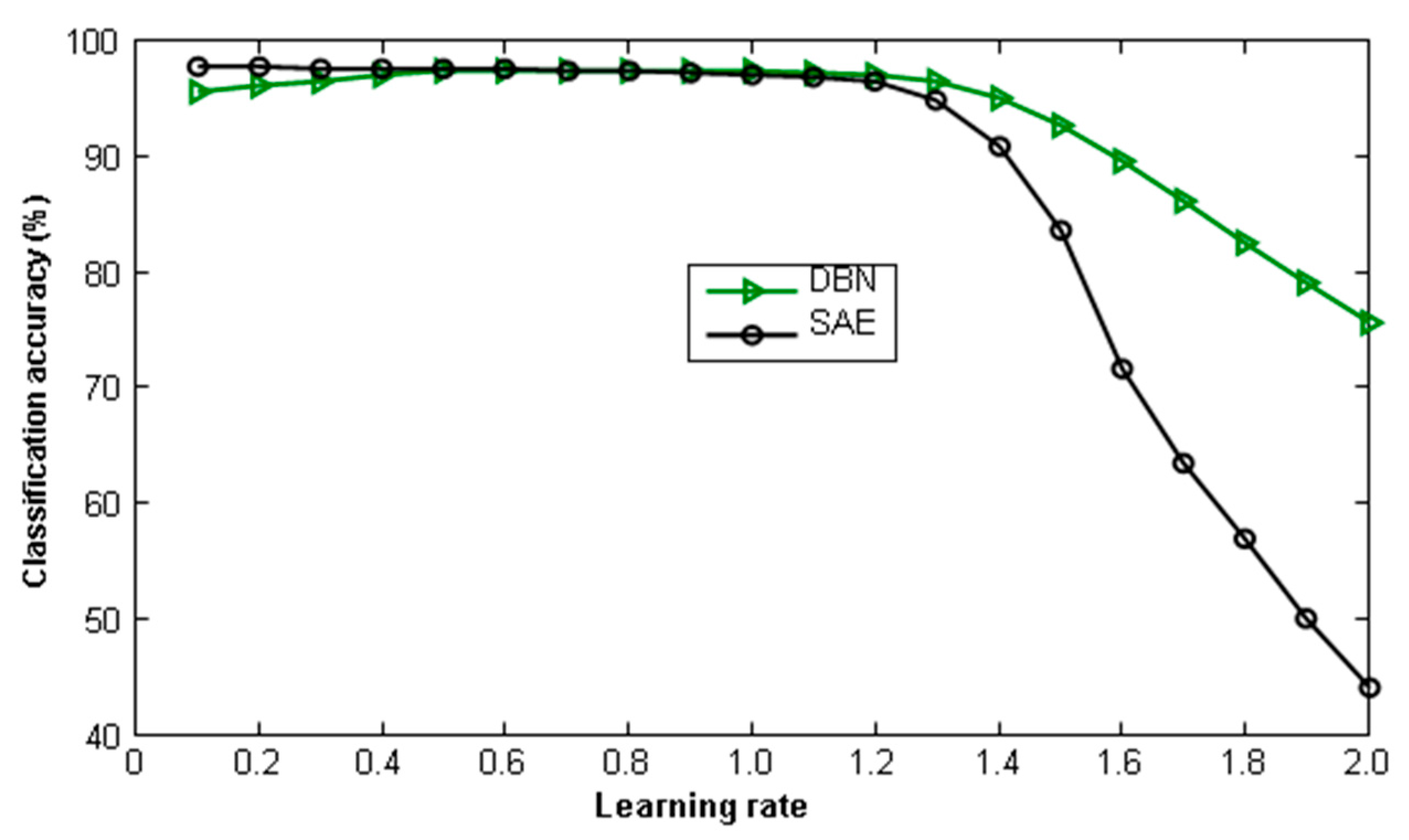
4.1.4. Learning Rate Choice
The learning rate is also called the step length, which refers to the scaling factor used to change each network weight. The selection of the learning rate has no theoretical guidance and can only be obtained by performing simulation experiments. When the learning rate is less than the ideal value, the algorithm can be guaranteed to converge to the global minimum but with a corresponding increase in training time. When the learning rate is much larger than the ideal value, the network cannot converge to the global minimum, even at the terminating cycle, and the training fails.
Figure 14 shows the depth of the two different ways of initialization-vector learning-network classification accuracy; it can be seen from the diagram that, based on the depth of the SAE learning vector of less than 1.1 and less than 1.2, and based on the depth of the DBN, learning classification accuracy is kept at a certain value. When the learning rate was greater than 1.1, network training failed. To save training time and ensure that the network converges, this paper selected 1 as the learning rate of this data set.
4.1.5. Relationship between Classification Accuracy and Fine Sample Size
Determination of the deep learning weights is divided into two steps. The first step is to modify the randomly generated weights determined by unsupervised learning of the original data, i.e., the initialization of the weights. The second step, through the study of the labeled data, is the overall adjustment of the weights after initialization, i.e., the weight adjustment. The successful solution to the training gradient diffusion problem was determined by layer by layer initialization. Since this involves unsupervised training, the weights determined in training can reflect the essential characteristics of the data. The different structures of deep learning are also shown here. Stack Auto-Encoding (SAE) is based on automatic encoding to initialize weights, and the degree of confidence is determined by the restricted Boltzmann machine. The weights of the two deep learning steps are in perfect alignment. Fine-tuning involves the study of labeled samples with the aim of improving the network’s separability of data; this process plays a vital role in the correct classification of unknown data.
To save training time and improve the ability of the network to be separable and as robust as possible, and to reduce the difficulty of data classification, the design of the experiment was such that the labeled samples had the same numerical proportions as the original data and did not classify the accuracy rate at the same time. The result in Figure 15 shows the classification accuracy of deep learning increases as the total sample proportion of fine-tuning samples (labeled sample) increases. When the proportion of labeled samples is more than 20%, the increase in classification accuracy slows. When the proportion of labeled samples is greater than 80%, the accuracy no longer increases with the number of labeled samples.
In addition, the classification accuracy of the deep learning algorithm is also related to the number of categories of patterns. As the number of categories increases, the classification accuracy is reduced accordingly. However, this problem can be overcome by increasing the number of training cycles. When the frequency of algorithm training is adjusted, the influence of class number on classification accuracy can be ignored. This approach is obviously better than the one with other algorithms, and it effectively overcomes the weaknesses of support vector machines in handling multiple classification problems.
4.2. Deep Learning Combined with Other Algorithms
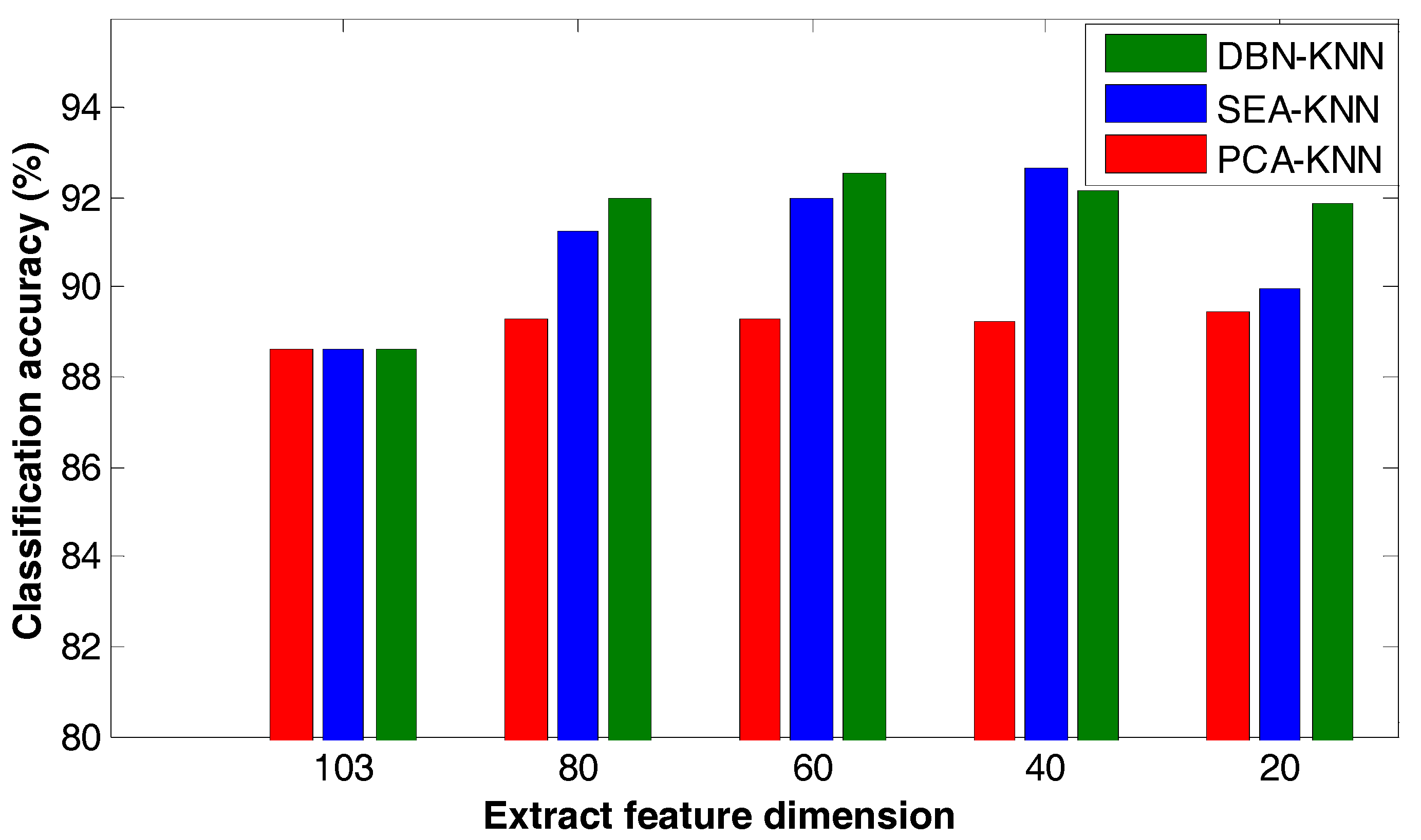
4.2.1. Contrast between Deep Learning and Principal Component Analysis
Principal component analysis is based on the concept of the data being linearly separable. By far the most popular way to solve the linear inseparability problem is by transforming the problem into a higher dimensional space, where it is linearly separable. The chief drawback of this method is it is computationally expensive and takes up more memory space. The method of deep learning by projection solves the problem of linear inseparability and saves more storage space than the nucleation method. In this simulation, two different algorithms for deep learning and principal component analysis were used to reduce the dimensionality of the spectral data of the University of Pavia and subsequently classify the data using the k-nearest neighbor algorithm. The results are shown in Figure 5.
Figure 16 shows the results when using the same classification algorithm and extracting the characteristics under the same conditions. Using principal component analysis (PCA) for compression to extract the characteristics yields the lowest classification accuracy. When using SAE and DBN the classification accuracy is higher. As seen from the figure, when extracting the feature, the classification accuracy is between 80 and 40 percent. The other two data compression methods using SAE and DBN need training. And after network training, the classification processing is significantly faster than with PCA.
4.2.2. Comparison of Deep Learning and Other Algorithm Classification Results
Different algorithms have different advantages. Naive Bayes (NBM) and k-nearest neighbor (KNN) algorithms do not require training: when the data is simple, their reliability is high. SVM can achieve better classification results with a small number of labeled samples. However, these traditional algorithms cannot achieve better classification results for spectral data with a large number of dimensions and a small sample size, and when the data is linearly inseparable. Table 1 shows the classification of high-dimensional spectral data of the University of Pavia.
The runtime and memory usage of the deep learning and support vector machines shown in Table 1 are based on trained networks. Of the five algorithms, only two deep learning networks and SVM have more than 90% classification accuracy; the memory usage and running time of SVM are larger than that of deep learning. As seen by repeated experimentation, deep learning for processing hyperspectral data has obvious time and memory usage advantages. In addition, deep learning is more accurate and stable than other algorithms. The classification accuracy of SAE-LR is slightly higher than that of DBN-LR for high dimensional spectral data used in this simulation.
4.2.3. Deep Learning Extracts Features and Results are Compared with Other Algorithms
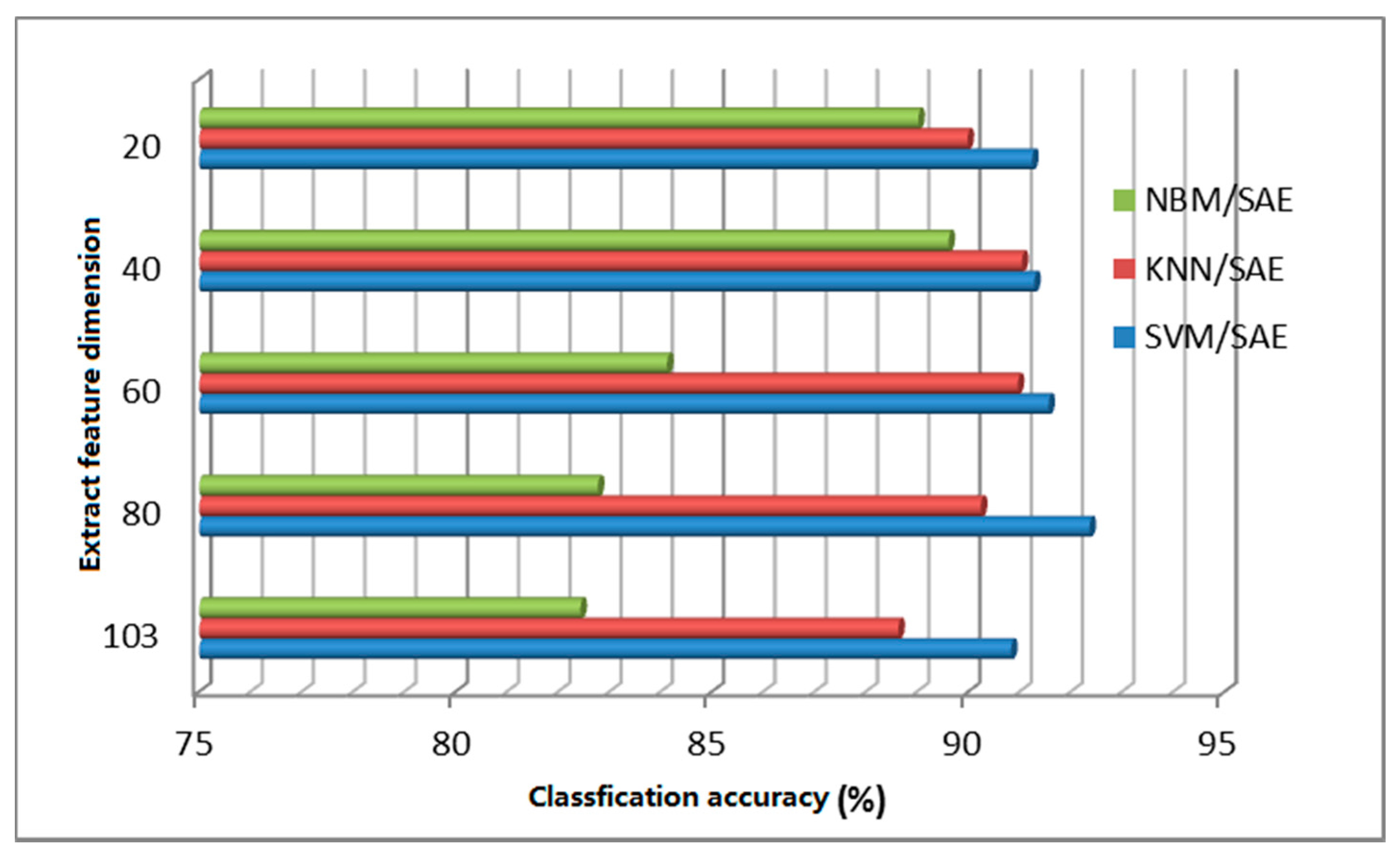
The deep learning algorithm can be regarded as logical regression (LR) for classifying the object characteristics after segmentation. Formally, there are two layers of neural networks. The feature of deep learning extraction is that it can describe the nature of the raw data beyond the features extracted using other data compression algorithms. In theory, using the SVM classification for data compressed by deep learning can obtain better classification results and can effectively save computer hardware resources and avoid problems such as the curse of dimensionality. This paper proposes an improved algorithm for data reduction based on deep learning. Figure 17 and Figure 18 are the classification results of the improved classification algorithm based on a confidence network and a stack automatic coding network.
As seen from Figure 17 and Figure 18, after stack automatic encoding or dimensional reduction of the data, the classification precision of the other traditional classification algorithms is significantly higher than with processing of the original data. SVM has the highest classification accuracy, followed by k-nearest neighbor and then by Naive Bayes, with the lowest classification accuracy. Naive Bayes achieves higher classification accuracy when working with compressed data (in Figure 17 a dimension 20 achieved the highest classification accuracy of 89.7%; in Figure 18, when dimension was 40, the classification accuracy increased to 88.92%), and SVM classification accuracy using compressed data with a dimension 80 achieved the highest accuracy.
4.3. Algorithm Verification
In addition, the dimensionality of the original data is reduced using the deep-belief algorithm, and the results are then classified using other algorithms. This can shorten training time and assure accuracy. When the fine-tuning sample size is 50, the classification accuracy of the different classification algorithms after dimensional reduction is shown in Table 2.
When the labeled sample size is small, the change of classification accuracy using different algorithms, along with the labeled sample size, is shown in Table 3.
As shown in Table 2, KNN and NBM do not need training; SVM need to train directly using the tagged samples; DNN-LR and DNN-SOM are first initialized with unlabeled samples, and then fine-tuned with labeled samples. Table 1 illustrates that for the data set, the classification accuracy of the other algorithms in the case of few labels is lower than that of deep learning algorithms. However, deep learning network parameters are obtained by unsupervised training, so the accuracy of DNN-LR and DNN-SOM is high. In addition to the proposed algorithm, the classification accuracy of other algorithms increases as the label sample size increases. For the label sample sizes of 12 and 24, the classification accuracy of the deep belief self-organizing neural network is the highest. When the sample size is large, the data show that the proposed algorithm is not dominant.
5. Conclusions
In the case of a small labeled sample size, the classification accuracy using a deep belief network algorithm is higher than that obtained using other algorithms. In addition, characteristics using the deep belief net can match the original spectral data notably well. Other classification algorithms can also achieve high classification accuracy. To a certain extent, this method can solve the hyperspectral data linear inseparability problem. However, when the number of labeled samples is small, the semi-supervised classification accuracy of this algorithm still needs to be improved. Although using a deep belief net for the dimensional reduction of the data can solve the problem of the self-organizing neural network training time to a certain degree, the training time needs to be shortened to be comparable with other semi-supervised classification algorithms.
Acknowledgments
The authors are supported by the Chinese National Natural Science Foundation (No. 61773039), Aerospace Science and technology group fund for science and technology, (No. KZ3XX19101), ‘Fanzhou’ Youth Scientific Funds (No. 20100504), and the Fundamental Research Funds for the Central Universities (No. YWF-14-HKXY-017, YWF-13-HKXY-033).
Author Contributions
Conceptualization: Wei Lan. Data curation: Wei Lan, Suling Jia. Formal analysis: Ke Li, Qingjian Li, Nan Yu. Funding acquisition: Ke Li. Investigation: Ke Li. Methodology: Wei Lan, Ke Li. Project administration: Wei Lan, Ke Li. Resources: Ke Li. Software: QingJian Li, Nan Yu, QuanXin Wang. Supervision: Ke Li. Validation: Ke Li, Wei Lan. Visualization: Ke Li, Wei Lan. Writing original draft: Wei Lan, Ke Li. Writing review and editing: Ke Li, Wei Lan.
Conflicts of Interest
The authors declare no conflict of interest.
References
- Xu, H.; Wang, X. Applications of multispectral/hyperspectral imaging technologies in military. Infrared Laser Eng. 2007, 36, 13–17. (In Chinese) [Google Scholar]
- Li, J.; Rao, X.; Ying, Y.; Wang, D. Detection of navel oranges canker based on hyperspectral imaging technology. Trans. Chin. Soc. Agric. Eng. 2010, 26, 222–228. (In Chinese) [Google Scholar]
- Melgani, F.; Bruzzone, L. Classification of hyperspectral remote sensing images with support vector machines. IEEE Trans. Geosci. Remote Sens. 2004, 42, 1778–1790. [Google Scholar] [CrossRef]
- Huang, M.; He, C.; Zhu, Q.; Qin, J. Maize Seed Variety Classification Using the Integration of Spectral and Image Features Combined with Feature Transformation Based on Hyperspectral Imaging. Appl. Sci. 2016, 6, 183. [Google Scholar] [CrossRef]
- Li, J.; Bioucas-Dias, J.M.; Plaza, A. Semisupervised hyperspectral image segmentation using multinomial logistic regression with active learning. IEEE Trans. Geosci. Remote Sens. 2010, 48, 4085–4098. [Google Scholar] [CrossRef]
- Harsanyi, J.C.; Chang, C.I. Hyperspectral image classification and dimensionality reduction: An orthogonal subspace projection approach. IEEE Trans. Geosci. Remote Sens. 1994, 32, 779–785. [Google Scholar] [CrossRef]
- Lee, M.; Prasad, S.; Bruce, L.M.; West, T.R.; Reynolds, D.; Irby, T.; Kalluri, H. Sensitivity of hyperspectral classification algorithms to training sample size. In Proceedings of the IEEE First Workshop on Hyperspectral Image and Signal Processing: Evolution in Remote Sensing (WHISPERS’09), Grenoble, France, 26–28 August 2009; pp. 1–4. [Google Scholar]
- Demir, B.; Ertürk, S. Hyperspectral image classification using relevance vector machines. IEEE Geosci. Remote Sens. Lett. 2007, 4, 586–590. [Google Scholar] [CrossRef]
- Gualtieri, J.A.; Cromp, R.F. Support vector machines for hyperspectral remote sensing classification. In Proceedings of the 27th AIPR Workshop: Advances in Computer-Assisted Recognition, Washington, DC, USA, 14–16 October 1998; pp. 1–28. [Google Scholar]
- Liu, Y.; Li, K.; Huang, Y.; Wang, J.; Song, S.; Sun, Y. Spacecraft electrical characteristics identification study based on offline FCM clustering and online SVM classifier. In Proceedings of the 2014 International Conference on Multisensor Fusion and Information Integration for Intelligent Systems (MFI), Beijing, China, 28–30 September 2014; pp. 1–4. [Google Scholar] [CrossRef]
- Li, K.; Wu, Y.; Nan, Y.; Li, P.; Li, Y. Hierarchical multi-class classification in multimodal spacecraft data using DNN and weighted support vector machine. Neurocomputing 2017. [Google Scholar] [CrossRef]
- Li, K.; Wu, Y.; Song, S.; Sun, Y.; Wang, J.; Li, Y. A novel method for spacecraft electrical fault detection based on FCM clustering and WPSVM classification with PCA feature extraction. Proc. Inst. Mech. Eng. Part G J. Aerosp. Eng. 2017, 231, 98–108. [Google Scholar] [CrossRef]
- Li, K.; Liu, W.; Wang, J.; Huang, Y.; Liu, M. Multi-parameter decoupling and slope tracking control strategy of a large-scale high altitude environment simulation test cabin. Chin. J. Aeronaut. 2014, 27, 1390–1400. [Google Scholar] [CrossRef]
- Li, K.; Liu, W.; Wang, J.; Huang, Y. An intelligent control method for a large multi-parameter environmental simulation cabin. Chin. J. Aeronaut. 2013, 26, 1360–1369. [Google Scholar] [CrossRef]
- Li, K.; Liu, Y.; Wang, Q.; Wu, Y.; Song, S.; Sun, Y.; Liu, T.; Wang, J.; Li, Y.; Du, S. A Spacecraft Electrical Characteristics Multi-Label Classification Method Based on Off-Line FCM Clustering and On-Line WPSVM. PLoS ONE 2015, 10, e0140395. [Google Scholar] [CrossRef] [PubMed]
- Ratle, F.; Camps-Valls, G.; Weston, J. Semisupervised neural networks for efficient hyperspectral image classification. IEEE Trans. Geosci. Remote Sens. 2010, 48, 2271–2282. [Google Scholar] [CrossRef]
- Slavkovikj, V.; Verstockt, S.; De Neve, W.; Hoecke, S.V.; Walle, R.V.D. Hyperspectral Image Classification with Convolutional Neural Networks. In Proceedings of the 23rd Annual ACM Conference on Multimedia Conference, Brisbane, Australia, 26–30 October 2015; pp. 1159–1162. [Google Scholar]
- Chen, Y.; Lin, Z.; Zhao, X.; Wang, G.; Gu, Y. Deep learning-based classification of hyperspectral data. IEEE J. Sel. Top. Appl. Earth Observ. Remote Sens. 2014, 7, 2094–2107. [Google Scholar] [CrossRef]
- Tarabalka, Y.; Fauvel, M.; Chanussot, J.; Benediktsson, J.A. SVM-and MRF-based method for accurate classification of hyperspectral images. IEEE Geosci. Remote Sens. Lett. 2010, 7, 736–740. [Google Scholar] [CrossRef]
- Yang, C.; Everitt, J.H.; Bradford, J.M. Bradford yield estimation from hyperspectral imagery using spectral angle mapper (SAM). Trans. ASABE 2008, 51, 729–737. [Google Scholar] [CrossRef]
- Ma, X.L.; Ren, Z.Y.; Wang, Y.L. Research on Hyperspectral Remote Sensing Image Classification Based on SAM. Syst. Sci. Compr. Stud. Agric. 2009, 2, 0204–0207. [Google Scholar]
- Martinez, A.M.; Kak, A.C. PCA versus LDA. IEEE Trans. Pattern Anal. Mach. Intell. 2001, 23, 228–233. [Google Scholar] [CrossRef]
- Chang, C.I.; Wang, S. Constrained band selection for hyperspectral imagery. IEEE Trans. Geosci. Remote Sens. 2006, 44, 1575–1585. [Google Scholar] [CrossRef]
- Pompilio, L.; Pepe, M.; Pedrazzi, G.; Marinangeli, L. Informational Clustering of Hyperspectral Data. IEEE J. Sel. Top. Appl. Earth Observ. Remote Sens. 2014, 6, 2209–2223. [Google Scholar] [CrossRef]
- Marlin, B.M.; Swersky, K.; Chen, B.; Freitas, N.D. Inductive Principles for Restricted Boltzmann Machine Learning. J. Mach. Learn. Res. 2010, 9, 509–516. [Google Scholar]
- Fauvel, M.; Benediktsson, J.A.; Chanussot, J.; Sveinsson, J.R. Spectral and spatial classification of hyperspectral data using SVMs and morphological profiles. IEEE Trans. Geosci. Remote Sens. 2008, 46, 3804–3814. [Google Scholar] [CrossRef]
- Zhao, X.; Wang, W.; Chu, X.; Li, C.; Kimuli, D. Early Detection of Aspergillus parasiticus Infection in Maize Kernels Using Near-Infrared Hyperspectral Imaging and Multivariate Data Analysis. Appl. Sci. 2017, 7, 90. [Google Scholar] [CrossRef]
- Lin, Z.; Chen, Y.; Zhao, X.; Wang, G. Spectral-spatial classification of hyperspectral image using autoencoders. In Proceedings of the IEEE 2013 9th International Conference on Information, Communications and Signal Processing (ICICS), Tainan, Taiwan, 10–13 December 2013; pp. 1–5. [Google Scholar]
- Djokam, M.; Sandasi, M.; Chen, W.; Viljoen, A.; Vermaak, I. Hyperspectral Imaging as a Rapid Quality Control Method for Herbal Tea Blends. Appl. Sci. 2017, 7, 268. [Google Scholar] [CrossRef]
- Zou, Q.; Ni, L.; Zhang, T.; Wang, Q. Deep Learning Based Feature Selection for Remote Sensing Scene Classification. IEEE Geosci. Remote Sens. Lett. 2015, 12, 2321–2325. [Google Scholar] [CrossRef]
- Fischer, A.; Igel, C. Training restricted Boltzmann machines: An introduction. Pattern Recognit. 2014, 47, 25–39. [Google Scholar] [CrossRef]
- Lefcourt, A.; Kistler, R.; Gadsden, S.; Kim, M. Automated Cart with VIS/NIR Hyperspectral Reflectance and Fluorescence Imaging Capabilities. Appl. Sci. 2016, 7, 3. [Google Scholar] [CrossRef]
- Bengio, Y. Learning Deep Architectures for AI. Found. Trends Mach. Learn. 2009, 2, 1–127. [Google Scholar] [CrossRef]
- Bengio, Y.; Lamblin, P.; Popovici, D.; Larochelle, H. Greedy layer-wise training of deep networks. In Proceedings of the International Conference on Neural Information Processing Systems, Vancouver, BC, Canada, 4–7 December 2006; pp. 153–160. [Google Scholar]
- Pal, M.; Foody, G.M. Feature selection for classification of hyperspectral data by SVM. IEEE Trans. Geosci. Remote Sens. 2010, 48, 2297–2307. [Google Scholar] [CrossRef]
- Shao, H.; Lam, W.H.K.; Tam, M.L. A reliability-based stochastic traffic assignment model for network with multiple user classes under uncertainty in demand. Netw. Spat. Econ. 2006, 6, 173–204. [Google Scholar] [CrossRef]
- Fischer, A.; Igel, C. An introduction to restricted Boltzmann machines. In Iberoamerican Congress on Pattern Recognition; Lecture Notes in Computer Science; Springer: Berlin, Heidelberg, 2012; pp. 14–36. [Google Scholar]
- Xu, P.; Xu, S.; Yin, H. Application of self-organizing competitive neural network in fault diagnosis of suck rod pumping system. J. Pet. Sci. Eng. 2007, 58, 43–48. [Google Scholar] [CrossRef]
- Tieleman, T. Training restricted Boltzmann machines using approximations to the likelihood gradient. In Proceedings of the International Conference on Machine Learning, Helsinki, Finland, 5–9 July 2008; pp. 1064–1071. [Google Scholar]
Figure 1.
Flowchart of the algorithm.

Figure 2.
Flowchart of the training.
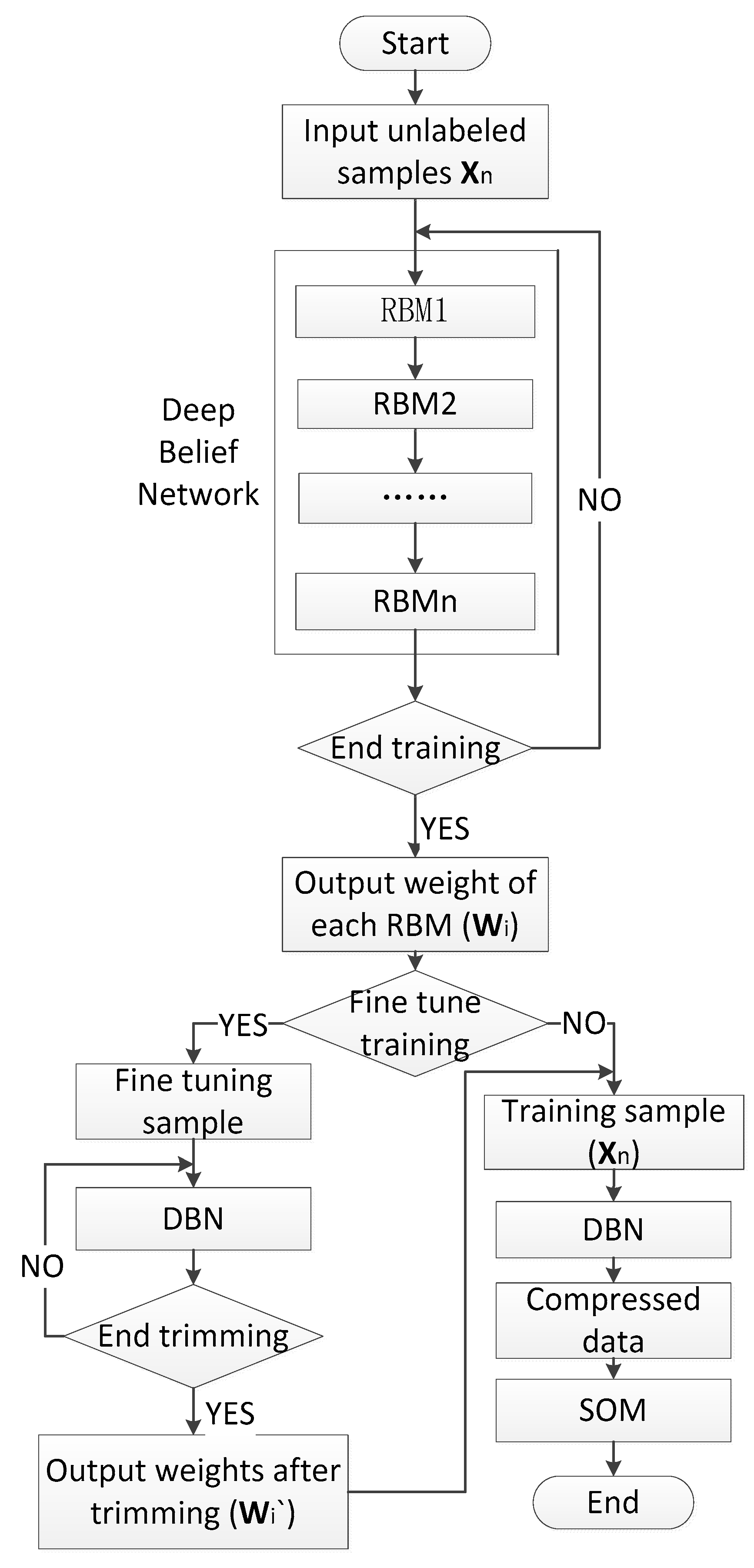
Figure 3.
Network topology of Restricted Boltzmann Machine.

Figure 4.
Topology of the self-organizing neural network.

Figure 5.
Hyperspectral data of Pavia University.

Figure 6.
Chart of the divisibility of data changes with the labeled samples.

Figure 7.
Classification accuracy varying with the labeled sample.

Figure 8.
Pavia Image. (a) Classification map based on Deep Belief Networks (DBN) and Self-Organizing feature Map (SOM). (b) Reference data.
Figure 8.
Pavia Image. (a) Classification map based on Deep Belief Networks (DBN) and Self-Organizing feature Map (SOM). (b) Reference data.
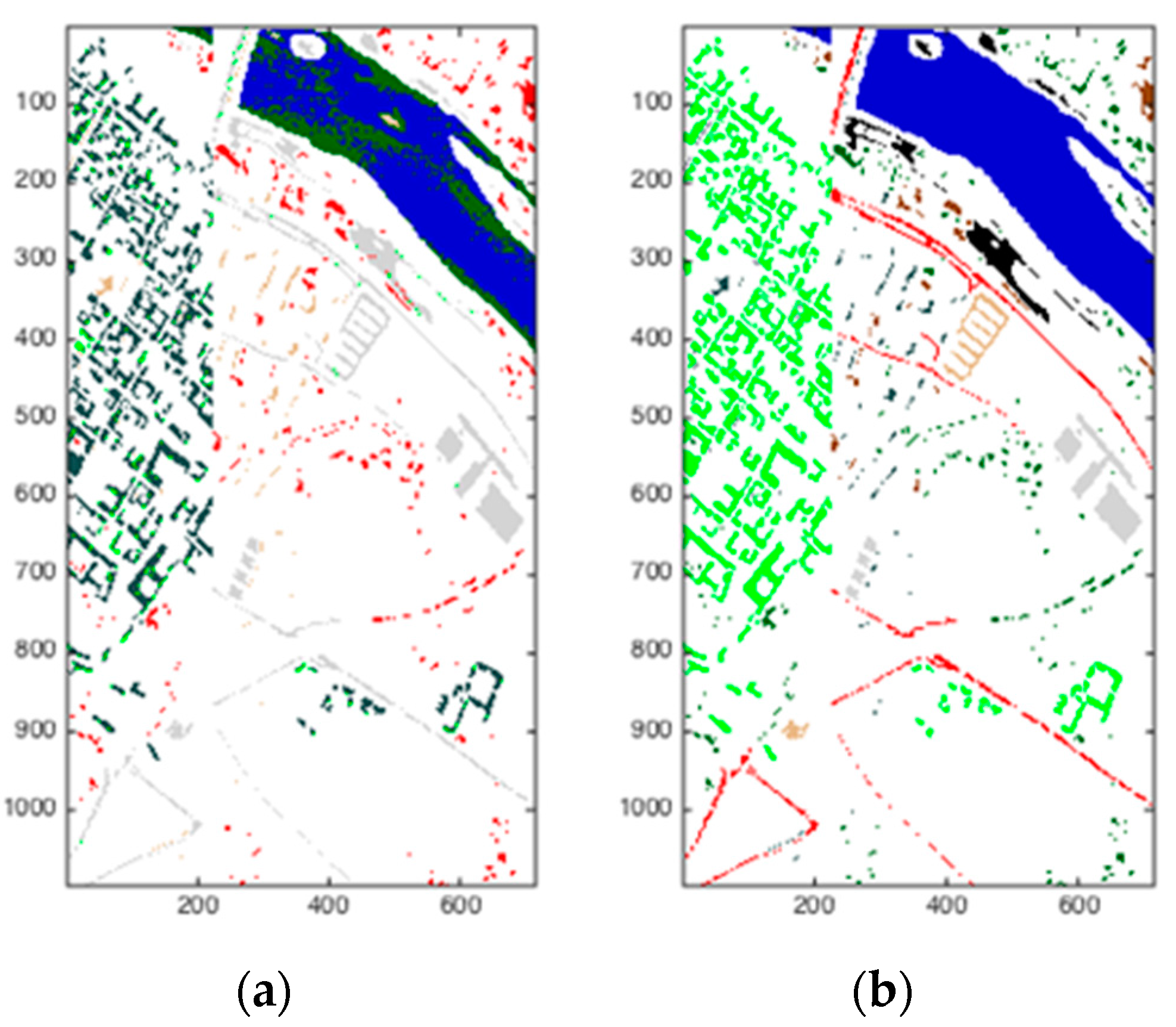
Figure 9.
Pavia University. (a) Classification map based on DBN and SOM; (b) Reference data.
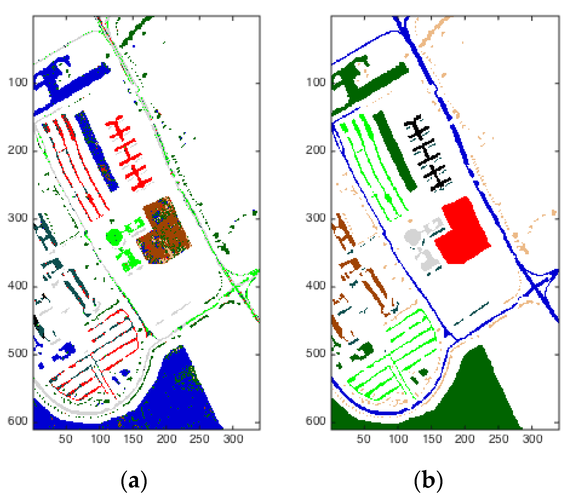
Figure 10.
Sanilas Image. (a) Classification map based on DBN and SOM. (b) Reference data.

Figure 11.
The high spectral data curve of the university of Pavia.

Figure 12.
The classification accuracy of different network depths varies with training cycles.

Figure 13.
The total error of classification varies with the number of cycles.

Figure 14.
Classification accuracy with learning rate variation.

Figure 15.
The classification accuracy is changed with the fine-tuning sample size.
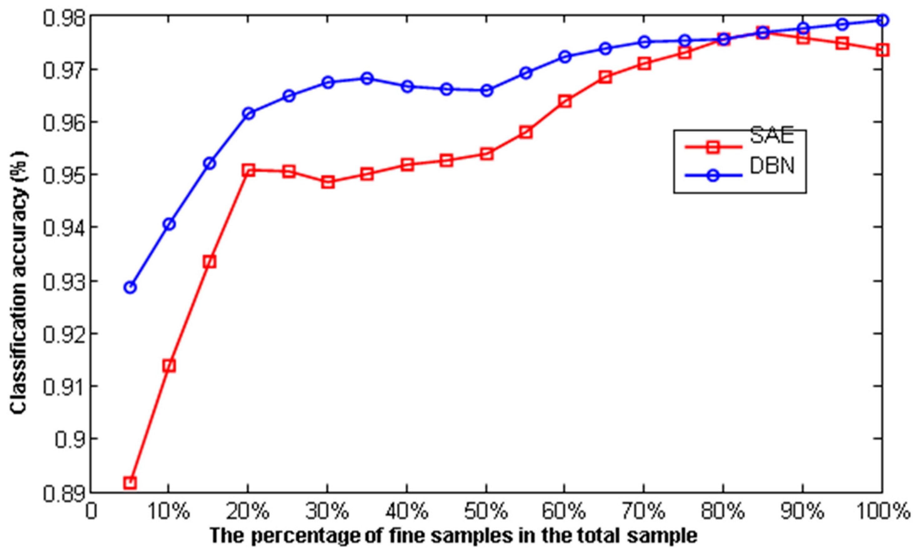
Figure 16.
Comparison of depth learning and principal component analysis.

Figure 17.
The classification accuracy of Deep Belief Networks (DBN) based on depth learning and other algorithms.
Figure 17.
The classification accuracy of Deep Belief Networks (DBN) based on depth learning and other algorithms.
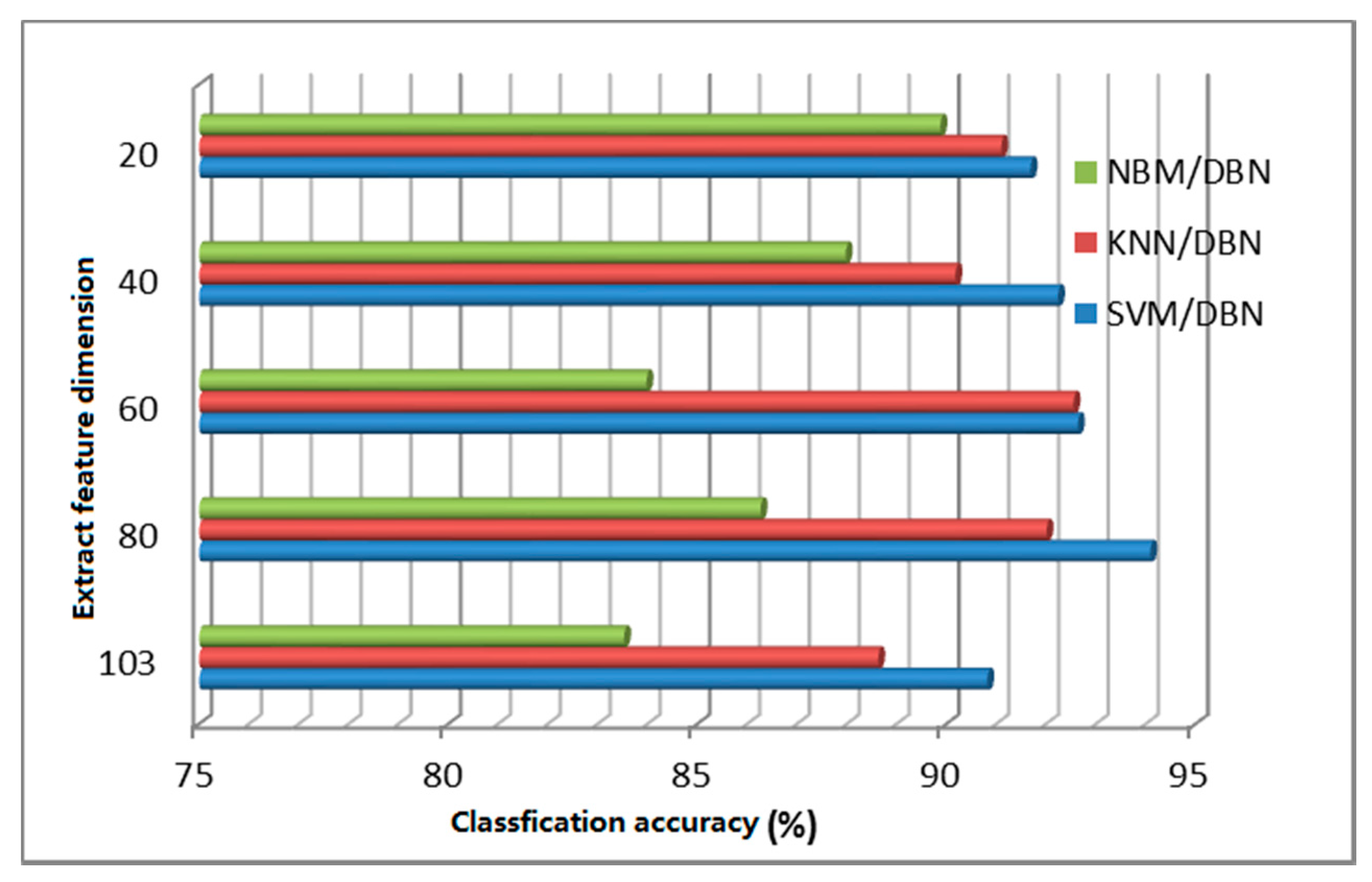
Figure 18.
The classification accuracy of Stack Auto-Encoding (SAE)-based depth learning and other algorithms.
Figure 18.
The classification accuracy of Stack Auto-Encoding (SAE)-based depth learning and other algorithms.

Table 1.
Classification accuracy of different classification algorithms.
| Classification Method | Classification Accuracy (%) | Memory Usage (MB) | Time Spent (s) |
|---|---|---|---|
| SAE-LR | 93.69 | 37 | 0.79 |
| DBN-LR | 92.87 | 35 | 0.53 |
| PCA-NBM | 88.08 | 39 | 28.054 |
| KNN | 88.66 | 126 | 3.713 |
| SVM | 90.84 | 76 | 5.99 |
Table 2.
Classification accuracy and training time variation chart for dimension reduction data.
| Methods | Accuracy of Compressed Data | Classification Time of Raw Data | Classification Time of Compressed Data |
|---|---|---|---|
| KNN | 89.53% | 40.825 s | 20.097 s |
| NBM | 86.45% | 115.11 s | 60.11 s |
| SVM | 89.7% | 30.297 s | 10.513 s |
Table 3.
Accuracy of different algorithms varies with the sample of the labeled sample.
| Methods | Labeled Sample 12 | Labeled Sample 24 | Labeled Sample 36 | Labeled Sample 50 |
|---|---|---|---|---|
| KNN | 73.50% | 82.71% | 84.50% | 85.38% |
| NBM | 71.21% | 79.95% | 81.13% | 86.32% |
| SVM | 76.76% | 81.92% | 85.45% | 85.72% |
| DNN-LR | 78.04% | 80.80% | 88.18% | 89.99% |
| DNN-SOM | 83.60% | 84.13% | 85.31% | 86.43% |
© 2017 by the authors. Licensee MDPI, Basel, Switzerland. This article is an open access article distributed under the terms and conditions of the Creative Commons Attribution (CC BY) license (http://creativecommons.org/licenses/by/4.0/).
Share and Cite
MDPI and ACS Style
Lan, W.; Li, Q.; Yu, N.; Wang, Q.; Jia, S.; Li, K. The Deep Belief and Self-Organizing Neural Network as a Semi-Supervised Classification Method for Hyperspectral Data. Appl. Sci. 2017, 7, 1212. https://doi.org/10.3390/app7121212
AMA Style
Lan W, Li Q, Yu N, Wang Q, Jia S, Li K. The Deep Belief and Self-Organizing Neural Network as a Semi-Supervised Classification Method for Hyperspectral Data. Applied Sciences. 2017; 7(12):1212. https://doi.org/10.3390/app7121212
Chicago/Turabian StyleLan, Wei, Qingjian Li, Nan Yu, Quanxin Wang, Suling Jia, and Ke Li. 2017. "The Deep Belief and Self-Organizing Neural Network as a Semi-Supervised Classification Method for Hyperspectral Data" Applied Sciences 7, no. 12: 1212. https://doi.org/10.3390/app7121212
Note that from the first issue of 2016, this journal uses article numbers instead of page numbers. See further details here.