A 3D Skeletonization Algorithm for 3D Mesh Models Using a Partial Parallel 3D Thinning Algorithm and 3D Skeleton Correcting Algorithm

Abstract

A three-dimensional (3D) skeletonization algorithm extracts the skeleton of a 3D model and provides it for many applications, such as 3D model classification and identification. There are three major skeletonization methodologies used in the literature, distance transform field-based methods, Voronoi diagram-based methods, and thinning-based methods. However, the existing algorithms cannot preserve the connectivity of the skeletons of the 3D mesh models. In this paper, we propose a 3D skeletonization algorithm for 3D mesh models using a partial parallel thinning algorithm and a 3D skeleton correcting algorithm. The proposed algorithm uses pre-defined removing and recovering templates. The partial parallel 3D thinning algorithm separates 62 symmetrical removing templates into two groups based on symmetry. It thins a model with the templates of each group in each thinning procedure. The 3D skeleton correcting algorithm uses six correcting templates to inspect the disconnected voxels in the skeleton and corrects them. The experimental results show several comparisons of skeletons extracted by different skeletonization algorithms. The proposed algorithm can extract the skeleton of each branch of a model and preserve the connectivity.

1. Introduction

The development of three-dimensional (3D) printing technology has recently led to the explosive growth of 3D models. 3D printing services are therefore increasing rapidly [1,2]. However, the copyright infringement of 3D models has become an issue for the 3D printing ecosystem of product distribution websites, 3D scanning, and design-sharing [3,4]. To prevent the unauthorized use of copyrighted 3D models, we should find out which copyrighted 3D models which are distributed on the internet, thus, the issue of identification of 3D models remains.

Various methods of extracting 3D model features have been proposed by many researchers [5,6,7,8,9,10,11,12]. Because of the highly discriminative property of 3D skeleton-based features for 3D model representation, 3D skeleton-based approaches have attracted much attention [5,6,7,8,9,10]. A 3D skeleton is not only an abstraction of the model at the center-line of the model but also a compact representation of the model, which is used for shape description, 3D model identification, and many other applications. The skeletons preserve the geometric and topologic properties of 3D models and are useful for 3D model matching, recognition, and retrieval [8].

There are three major skeletonization methodologies used in the literature: distance transform field-based methods [13,14,15], Voronoi diagram-based methods [16,17,18], and thinning-based methods [19,20,21,22,23]. The field-based methods extract a skeleton with missing branches. The Voronoi diagram-based methods extract a great number of spurious skeletal branches that are not essential for compact representation of the model [8,16,17,18]. Moreover, the computations of the Voronoi diagram are a time consuming process. The thinning-based methods are faster than the Voronoi diagram-based methods and extract more detailed skeletons than do those extracted by the field-based methods [24].

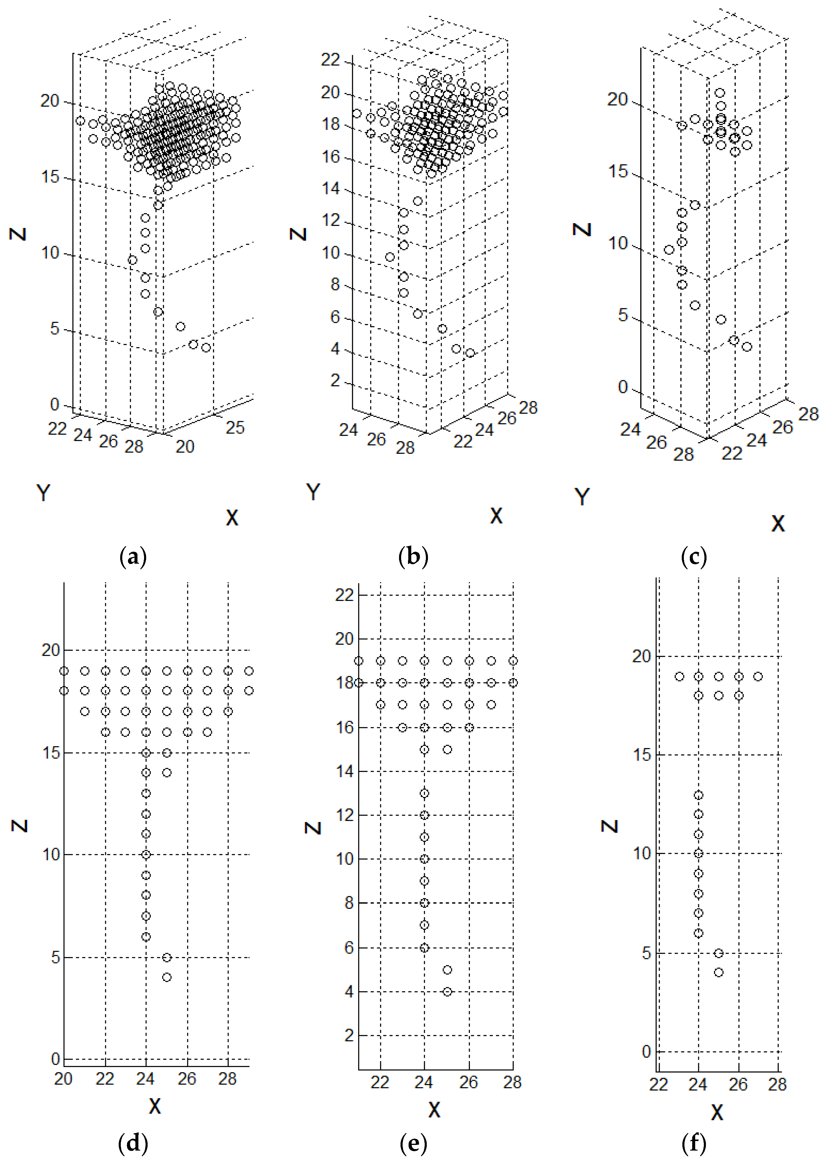
A thinning process is to erode an object’s surface layer by layer until only a skeleton remains. However, the existent thinning-based algorithms cannot preserve the connectivity of the skeletons of 3D mesh models. They accidentally remove some voxels that should be retained. Because they create new cavities and change the topology, an incorrect skeleton will be extracted. Figure 1 shows an example of removing a voxel that leads to the creation of a cavity during several continuous thinning procedures. To illustrate the disconnection more clearly, the figures are shown in a 3D and 2D xz-plane. Figure 1b,e shows a result after thinning the voxels in Figure 1a,d. They show that a cavity is created. Figure 1c,f shows a result after three times of thinning procedures. The cavity becomes larger, and the distance between the two separated branches becomes longer. The shape and topology of the skeleton are seriously damaged.

In [21], the authors modified and improved the fully parallel 3D thinning algorithm described in [22]. The fully parallel thinning algorithm is based on four types of removing templates (classes A, B, C, and D). The target voxel, which is the currently investigated voxel, will be removed if the neighborhoods of the target voxel match one of the templates and satisfies another criterion. However, the skeletons extracted by the modified algorithm may be disconnected when thinning the 3D mesh models.

A correct skeleton can increase the precision of skeleton-based 3D model identification. In the meantime, it can help to prevent copyrighted 3D models from being distributed illegally. Therefore, it is important to extract a correct skeleton. In this paper, we present a 3D skeletonization algorithm for 3D mesh models using a partial parallel thinning algorithm and a 3D skeleton correcting algorithm. The proposed algorithm uses pre-defined removing and recovering templates. The removing templates are derived from those proposed in [21]. The partial parallel 3D thinning algorithm separates 62 symmetrical removing templates to two groups based on symmetry. It thins a model with the templates of one group in each thinning procedure. The 3D skeleton correcting algorithm uses six correcting templates to inspect the disconnected voxels in the skeleton and corrects them. The templates are used to inspect 26-adjacent voxels of a current target voxel after it was removed. The correcting algorithm recovers the target voxel based on the recovering templates and an additional criterion that addresses the distances between the 26-adjacent voxels. To obtain a unit-width (one voxel wide) skeleton, we apply a post-process called the valence-driven spatial median (VDSM) algorithm [24] to the extracted skeleton. Several comparisons of the skeletons extracted by different skeletonization algorithms are shown in the experimental results section. The experimental results show that the proposed algorithm can extract the skeleton of each branch of a model and preserve its connectivity.

The remainder of this paper is organized as follows. In Section 2, we discuss related work. A brief overview of the basic theory of the adjacencies in a 3D binary array is given in Section 3. The methodology of the partial parallel 3D thinning algorithm is described in Section 4. In Section 5, the 3D skeleton correcting algorithm is introduced. A short review of the VDSM algorithm is given in Section 6. The experimental results of skeletons extracted by the proposed method and other methods are shown in Section 7. Finally, we conclude with the proposed method in Section 8.

2. Related Work

A fully parallel 3D thinning algorithm was proposed in [22]. It thinned the model with four types of removing templates to extract the skeleton. However, the algorithm cannot preserve connectivity. The authors in [21] modified and improved the fully parallel 3D thinning algorithm. The 12 removing templates in class D were changed and extended to 36 templates. However, the skeletons extracted by the improved algorithm are still disconnected.

Another 3D thinning algorithm was proposed in [23]. The authors modified the original removing templates and added two new criteria to extract a voxel-wide skeleton. However, the algorithm removed too many voxels to preserve the connectivity and topology of the skeleton.

A robust approach to the arc skeletonization algorithm was proposed in [25]. The skeleton was expanded iteratively by adding new branches. A minimum-cost geodesic path was used to connect the farthest voxels to the skeleton. However, the algorithm was only used for tree-like models and is not suitable for characters or animal models.

In [16,17,18], Voronoi diagram-based skeletonization algorithms utilized a method of incremental construction to approximate the skeletons with Voronoi diagrams. They generate spurious branches and are time-consuming.

In [13], a subvoxel precise distance field was used as the input, and the authors employed a number of fast marching method propagations to extract the skeleton at subvoxel precision. The algorithm cannot extract the skeleton of each branch of a 3D model.

In [19,20], the authors used a thinning algorithm to extract the skeleton and rechecked eight subvoxels with non-overlapping neighborhoods in parallel. However, the extracted skeleton included some spurious branches.

A simple and robust thinning algorithm was developed on a discrete representation of objects as cell complexes in [26]. The key observation was to formulate a skeleton significance measure called medial persistence (MP), to guide thinning. It records the duration in which a discrete cell persists in an isolated form during the removing process. However, under the MP score of preserving connectivity, the extracted skeletons contain noises.

A method of generating a unit-width skeleton was proposed in [24]. The authors used a valence-driven spatial median (VDSM) algorithm and Dijkstra’s shortest path algorithm to compute the center of the crowded voxels and remove the voxels that are not on the shortest path between the center and an exit of the crowded region. The algorithm can be used as a post-process, which can be combined with another skeletonization algorithm.

3. Basic Theory

First of all, a voxelization process is performed to a 3D mesh model as in [27]. The 3D space of the voxels is transformed to a 3D binary array. Each voxel is denoted by 1 in the 3D binary array. A binary value of 0 means that there is no voxel.

Suppose there are two voxels, $p_1$ and $p_2$, with coordinates $\left(x_1,y_1,z_1\right)$ and $\left(x_2,y_2,z_2\right)$ in the 3D binary array. The Euclidean distance between $p_1$ and $p_2$ is defined as (1) [21].

$$d=\sqrt{{\left(x_1-x_2\right)}^2+{\left(y_1-y_2\right)}^2+{\left(z_1-z_2\right)}^2}$$

(1)

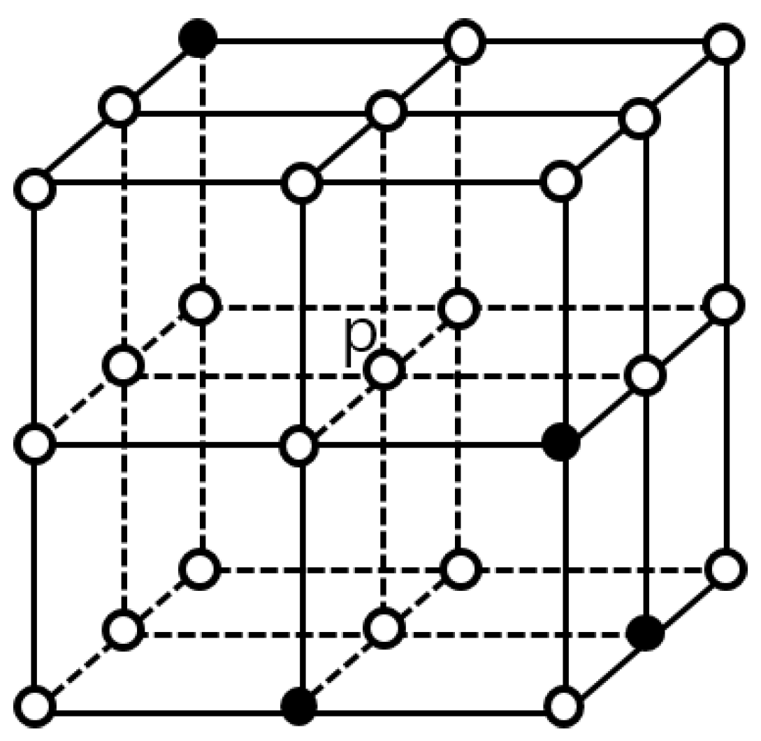
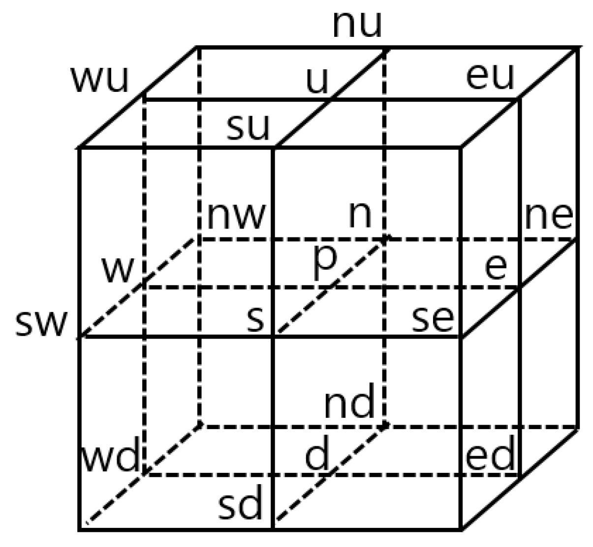
If $d=1$, then $p_1$ and $p_2$ are 6-adjacent. If $d\le \sqrt{2}$, then $p_1$ and $p_2$ are 18-adjacent. If $d\le \sqrt{3}$, then $p_1$ and $p_2$ are 26-adjacent. Figure 2 shows the adjacencies of a voxel $p$.

The n(p), e(p), s(p), w(p), u(p), and d(p) are six adjacent voxels of $p$, where the n, e, s, w, u, and d denote north, east, south, west, up, and down. The 18-adjacent voxels of $p$ (not including the 6-adjacent voxels) are nu(p), ne(p), nd(p), nw(p), eu(p), ed(p), su(p), se(p), sd(p), sw(p), wu(p), wd(p), etc.

4. 3D Partial Parallel Thinning Algorithm

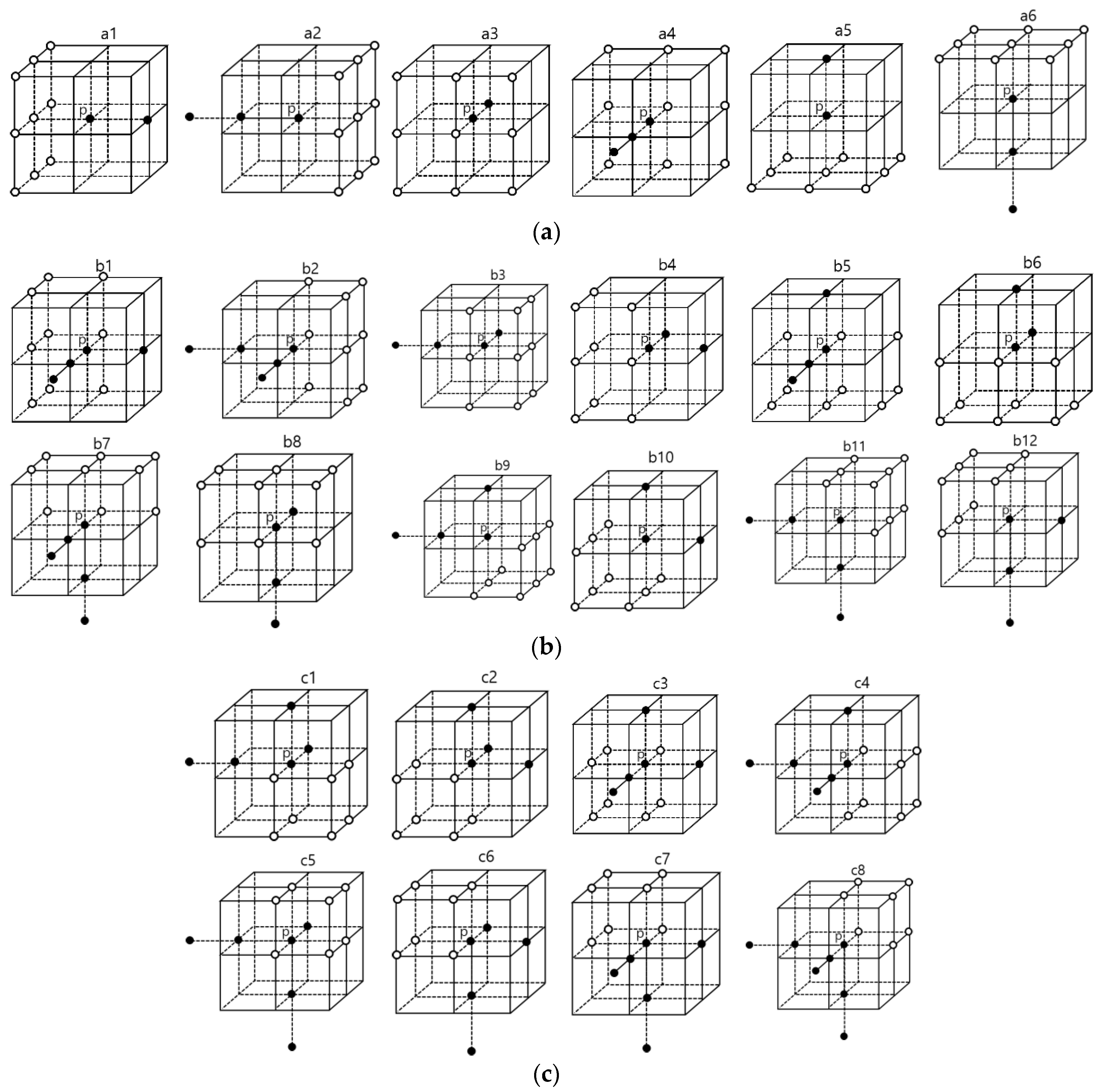
The parallel thinning algorithm is based on several pre-defined removing templates (class A, B, C, and D) [21,22]. The target voxel will be removed if the voxel is a non-tail voxel and the neighborhoods of the voxel match one of the templates.

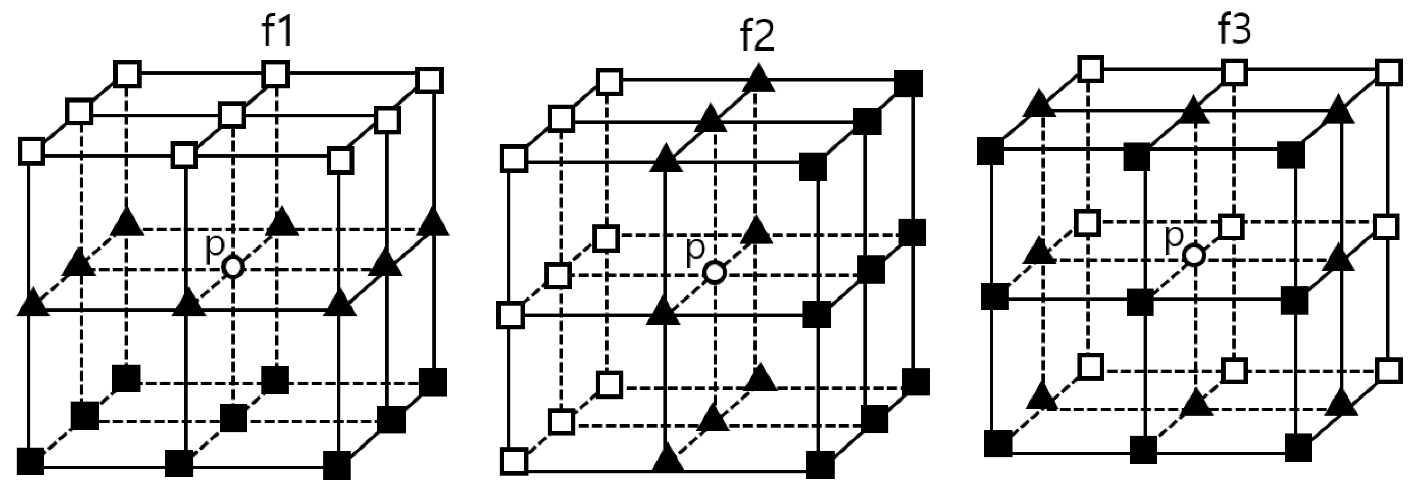
Figure 3 shows the templates of each class. There are six templates in class A, 12 templates in class B, 8 templates in class C, and 36 templates in class D. A solid black circle denotes a binary value 1, which means that a voxel exists. A white circle (background voxel) denotes a binary value 0, which means that there is no voxel. The voxels in the unmarked positions are ‘don’t care’ voxels, which means that the binary values can be either 1 or 0. The white squares mean that at least one of them is 1. The two white triangles in Figure 3d mean that both cannot be 1 simultaneously, which means that, at most, one of them is 1 or both of them are 0.

If a voxel $p$ is 26-adjacent to only one voxel, then it is called a line-end voxel. If the $p$ is 26-adjacent to only two voxels, then it is called a near-line-end voxel. If the $p$ is either a line-end or a near-line-end voxel, then it is called a tail voxel; otherwise, it is called a non-tail voxel. Analyze each voxel of a 3D model to determine whether it is a non-tail voxel and satisfies at least one of the removing templates of any class. After analyzing and marking the whole voxels, the voxels that satisfy both conditions will be removed simultaneously. Repeat the process until no voxel can be removed. The authors in [21] found that the 12 conventional templates of class D in [22] may disconnect the skeleton. Therefore, they modified and expanded each template of class D to three templates. Each of the templates from d1 to d6 in Figure 3d is expanded to three templates according to the binary values of the two triangles. There are thus 36 templates in class D. In [21], 18 templates were used to illustrate the templates from d1 to d6. However, in this paper, they are simplified to six templates by using the two triangles.

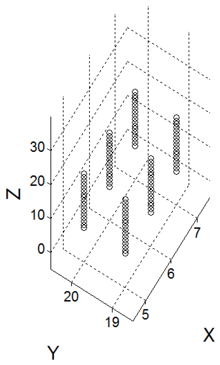
However, the fully parallel thinning algorithm has a drawback of thinning the voxels of pyramid structure. It removes each layer of voxels from the surface to the inside in each iteration and finally removes all voxels of pyramid structure. Figure 4 shows an example of the problem.

Figure 4a shows a portion of a manta ray model’s wing. Figure 4b shows a result after eight iterations of thinning procedures. After the ninth iteration, the whole voxels of the part are removed. The surface voxels of each layer are non-tail voxels and satisfy the removing templates. Therefore, the skeleton of the manta ray model’s wing cannot be extracted by the fully parallel thinning algorithm.

In [23], the templates are modified so that they are without any extended neighbors, which means that only the 26-adjacent voxels of the target voxel are considered for investigation. One of the two additional criteria is to determine whether any voxel in the 26-neighbors of the target voxel are 26-connected. If so, the target voxel is a candidate for removal. The other criterion is to determine whether any background voxel in the 18-neighbors of the target voxel is connected and contains at least one background 6-neighbor. If so, then the target voxel is considered for removal. However, this algorithm has the drawback of thinning the voxels with a structure as shown in Figure 5.

Figure 5 shows a lower part of the voxels of a model with the shape of the digit nine. The voxels satisfy the modified removing templates in class A and the two criteria. All voxels were therefore removed. If the templates are kept as in Figure 3, then the skeleton of this model can be extracted.

To solve the problem of removing all voxels, we separate the removing templates shown in Figure 3 into two groups based on symmetry. In class A, the templates a1, a3, and a5 are assigned to the first group, and a2, a4, and a6 are assigned to second group. They are symmetrical to each other. In class B, the templates b1, b2, b5, b6, b9, and b10 are assigned to the first group, and the others are assigned to the second group. In class C, the templates c1, c2, c3, and c4 are assigned to the first group, and the others are assigned to the second group. In class D, the templates d1, d2, d3, d4, d5, and d6 are assigned to the first group, and the others are assigned to the second group. During the thinning process, the templates in the first group are used to thin each odd-numbered iteration, and those in the second group are used for the even-numbered iterations. Figure 6 shows the result of thinning the same part of the manta ray model’s wing illustrated in Figure 4a. Figure 6a shows the result after 10 iterations of thinning procedures. Figure 6b shows the result after 20 iterations. The partial parallel thinning algorithm can keep the skeleton of the pyramid structure from being removed.

5. 3D Skeleton Correcting Algorithm

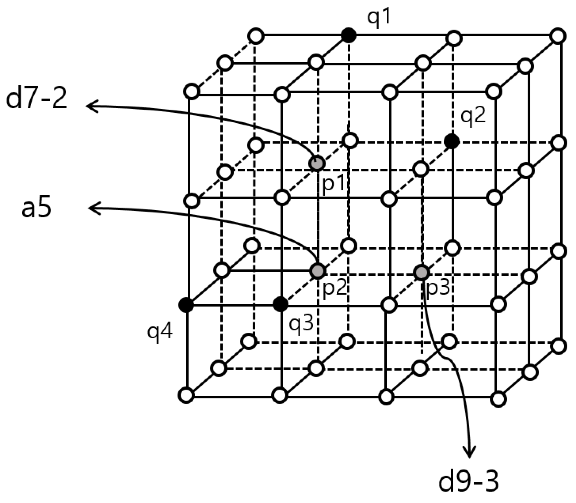
A 3D model thinning algorithm should keep the extracted skeleton connected. However, we found that the modified algorithm [21] failed to preserve connectivity. Figure 7 shows an example about how the algorithm disconnects the skeleton. The voxel p1 is a non-tail voxel because it is 26-adjacent to six voxels: p2, p3, q1, q2, q3, and q4. It also satisfies the template d7-2 in class D and will thus be removed. The voxel p2 is a non-tail voxel because it is 26-adjacent to five voxels: p1, p3, q2, q3, and q4. It also satisfies the template a5 in class A. Therefore, it will also be removed. The p3 voxel is a non-tail voxel because it is 26-adjacent to four voxels: p1, p2, q2, and q3. It also satisfies the template d9-3 in class D. Therefore, it will also be removed. When the voxels p1, p2, and p3 are removed, then the rest of the voxels are disconnected.

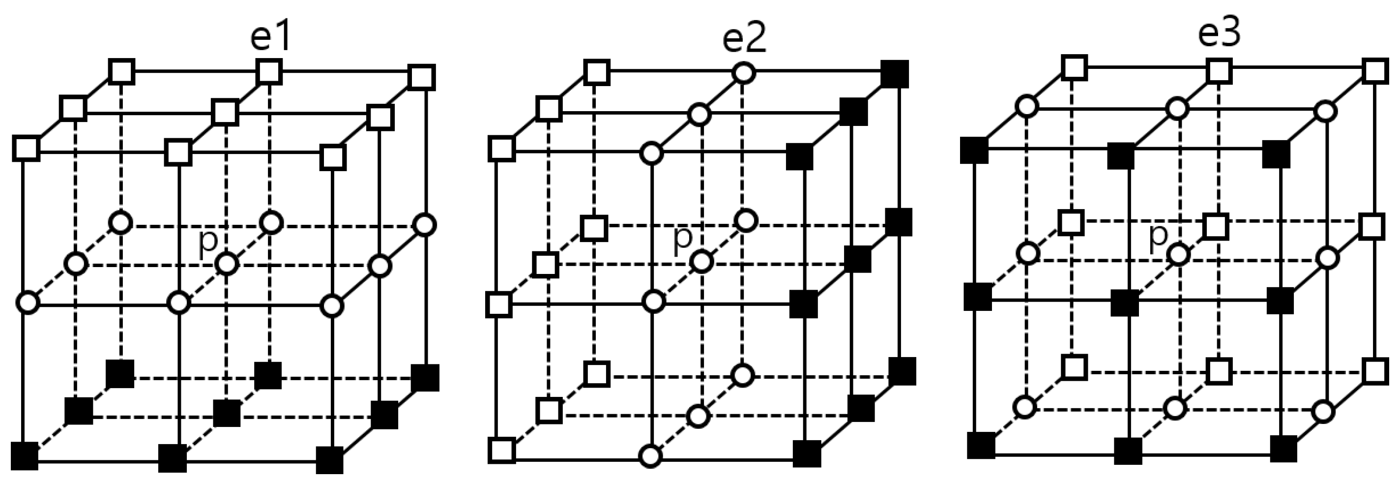
To preserve the connectivity of the skeleton, we propose a 3D skeleton correcting algorithm with six templates of inspecting the voxel disconnection. These templates are assigned to two classes: class E and class F. The templates in class E are shown in Figure 8. The black squares mean that at least one of them is 1. The templates in class E inspect the connectivity of the voxels by checking the distance between the voxels to determine whether it is greater than or equal to 2. After the target voxel p is removed, to satisfy the templates, the rest of the voxels are at the locations of both black squares and white squares. If the 26-adjacent voxels of the removed voxel satisfy the templates of class E, then the removed voxel p can be recovered. With the templates in class E, we can inspect whether voxels q1, q2, q3, and q4 in Figure 7 satisfy the template e3 after the last voxels of p1, p2, and p3 are removed. Thus, we can recover the last removed voxel to correct the disconnection of the skeleton and preserve connectivity.

Another example of disconnection is shown in Figure 9. This case occurs after the target voxel is removed by template d11-1. Obviously, the remainder of the voxels are separated into two parts, which lead to the creation of a cavity. In this case, the removed voxel cannot be recovered by the templates in class E. Therefore, we propose the other three templates of class F to address such a special case.

Figure 10 shows the templates in class F. The black triangles denote that at least one of them is 1. An additional criterion is employed to inspect the distances between the 26-adjacent voxels. We define the numbers of the voxels at the locations of white squares, black triangles and black squares as $n_{ws}$, $n_{bt}$, and $n_{bs}$. The set of distances between the voxels at the locations of the white squares and those at the black triangles are defined as $DW=\left\{d{w}_1,d{w}_2,\dots ,d{w}_M\right\},\left(M=n_{ws}\times n_{bt}\right)$. The set of distances between the voxels at the locations of black squares and those at the black triangles are defined as $DB=\left\{d{b}_1,d{b}_2,\dots ,d{b}_N\right\},\left(N=n_{bt}\times n_{bs}\right)$. The judgment of whether the target voxel will be recovered is defined as follows:

$$rc=\{\begin{array}{cc}\hfill false,& \mathrm{i}\mathrm{f} \mathrm{m}\mathrm{i}\mathrm{n}\left\{DW\right\}\le \tau and \mathrm{m}\mathrm{i}\mathrm{n}\left\{DB\right\}\le \tau \hfill \\ \hfill true,& otherwise\hfill \end{array}$$

(2)

The $\tau$ is a threshold value for checking the 26-adjacent voxels and is equal to $\sqrt{3}$. The target voxel will be recovered if the $rc$ has a true value. Therefore, the removed voxel can be recovered based on any template in class F and the additional criterion.

6. Process of Unit-Width Skeleton Based on Valence-Driven Spatial Median Algorithm

To obtain a unit-width skeleton, we use the VDSM algorithm to eliminate some crowded voxels and output a one-voxel wide skeleton [24]. The VDSM algorithm computes the valence (degree) of each voxel in the skeleton by counting the number of the 26-adjacent voxels. The degree of a voxel is defined as $D\left(p\right)$. If $D\left(p\right)=1$, then the voxel is called an end voxel. If $D\left(p\right)=2$, then the voxel is called a middle voxel. If $D\left(p\right)=n(n>2)$ and the 26-adjacent voxels are either middle voxels or end voxels, then the voxel is called a joint voxel. If a voxel is neither a joint voxel, a middle voxel, nor an end voxel, then the voxel is called a crowded voxel. A crowded region is composed of 26-connected crowded voxels. If a voxel is a middle voxel or an end voxel and is 26-connected to one crowded voxel, then it is called an exit. The VDSM algorithm marks every end voxel, middle voxel, joint voxel, crowded voxel, and exit to each crowded region. The next step is to find the center of each crowded region. A crowded region of $n$ crowded voxels is defined as $CR=\left\{c{v}_1,c{v}_2,\dots ,c{v}_n\right\}$. The center $c$ is then computed as follows:

$$c={\mathrm{argmin}}_i\left\{{\displaystyle \sum }_{j=1}^n\frac{1}{D\left(p\right)}{\left|c{v}_i-c{v}_j\right|}^2\right\}$$

(3)

Once the centers are obtained, the Dijkstra’s shortest path algorithm [28,29] is used to connect the centers and all of the corresponding exits. The crowded voxels outside the shortest paths will be removed. Finally, we can obtain the unit-width skeleton.

7. Experimental Results

In this section, we show some experimental results of extracting skeletons by different skeletonization algorithms. The proposed algorithm is compared with five other skeletonization algorithms. The first one was described in [13], which used fast marching methods (FMM). The second one was proposed in [19,20], which built a skeleton via the 3D medial surface and axis (MSA). The third one was proposed in [23], which modified the templates and added two additional criteria (MTTAC). The fourth one was proposed in [21,22], which used a fully parallel thinning algorithm (FPT). 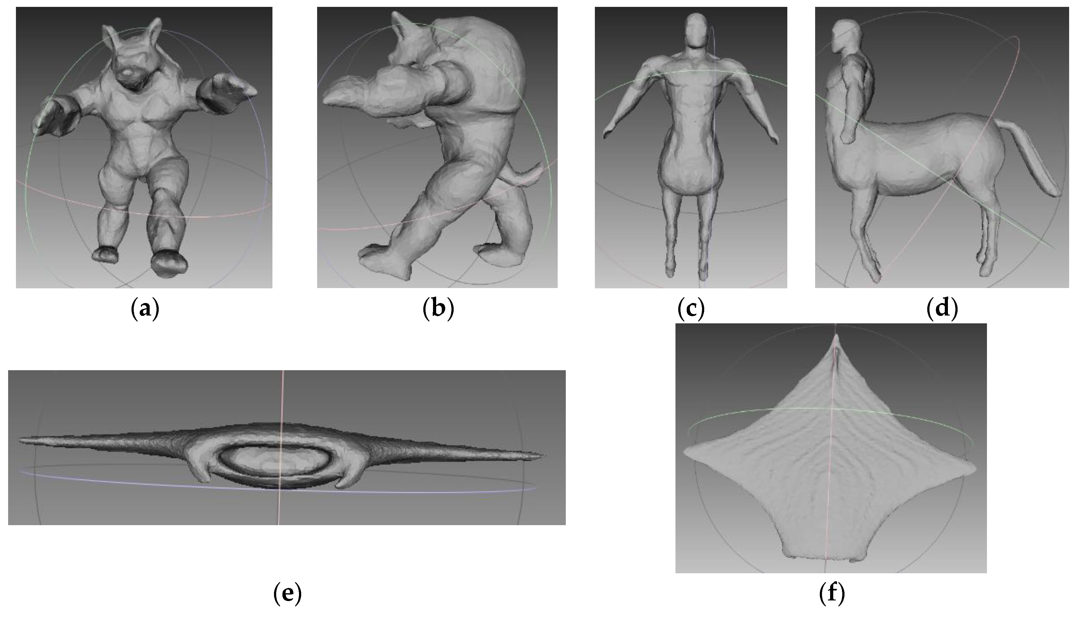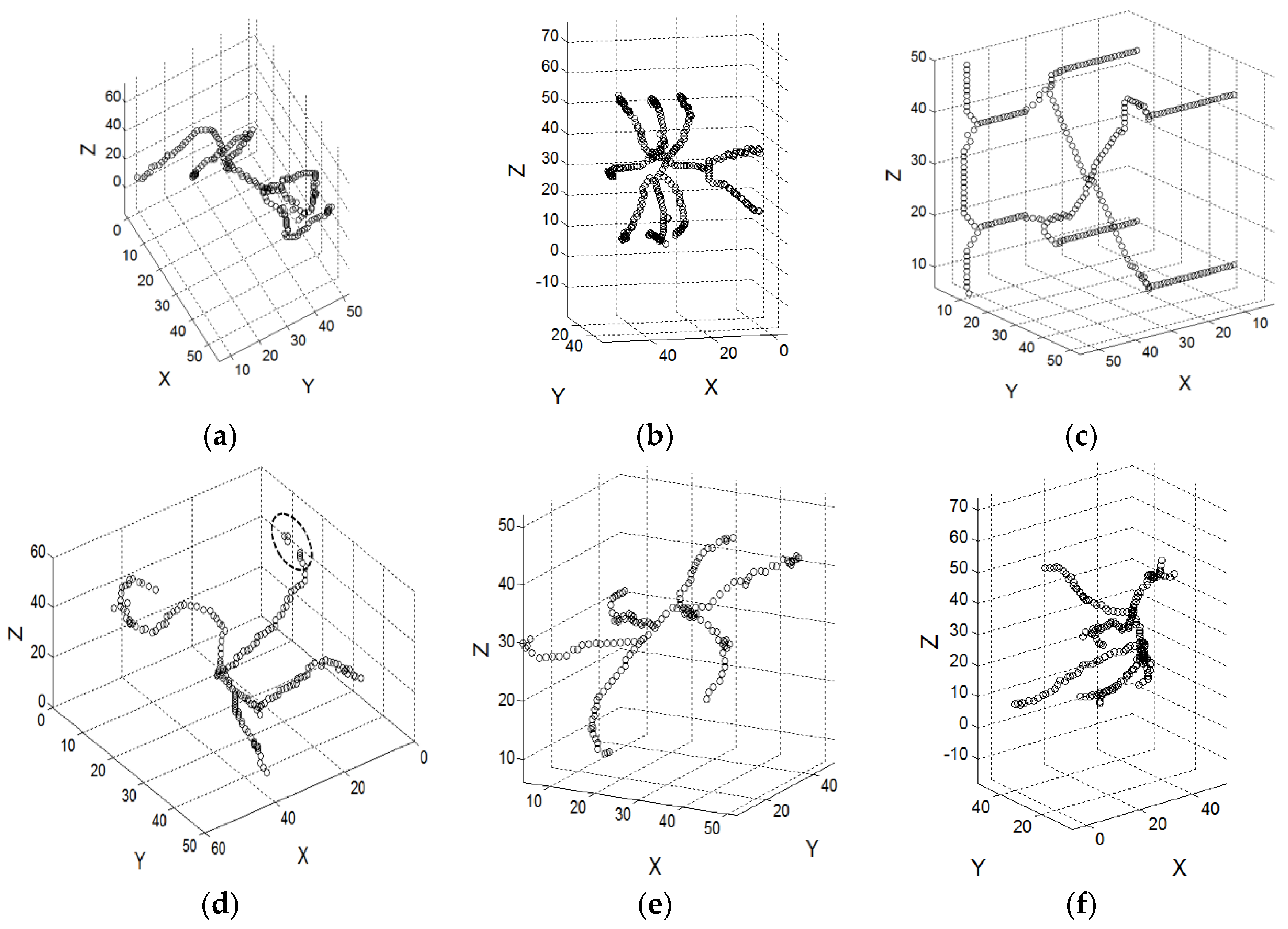The last one was proposed in [26], which used the cell complexes and medial persistence (CCMP). The performances of the algorithms were evaluated with 100 3D mesh models in the SHREC 2015 benchmark. We show comparison results of three representative models of animals and humans. Figure 11 shows the three models: armadillo, centaur, and manta ray. The numbers of the triangles are 17,656; 18,868; and 20,000, respectively. Before thinning the models, we first voxelized the mesh models to $50\times 50\times 50$ grids as in [27].

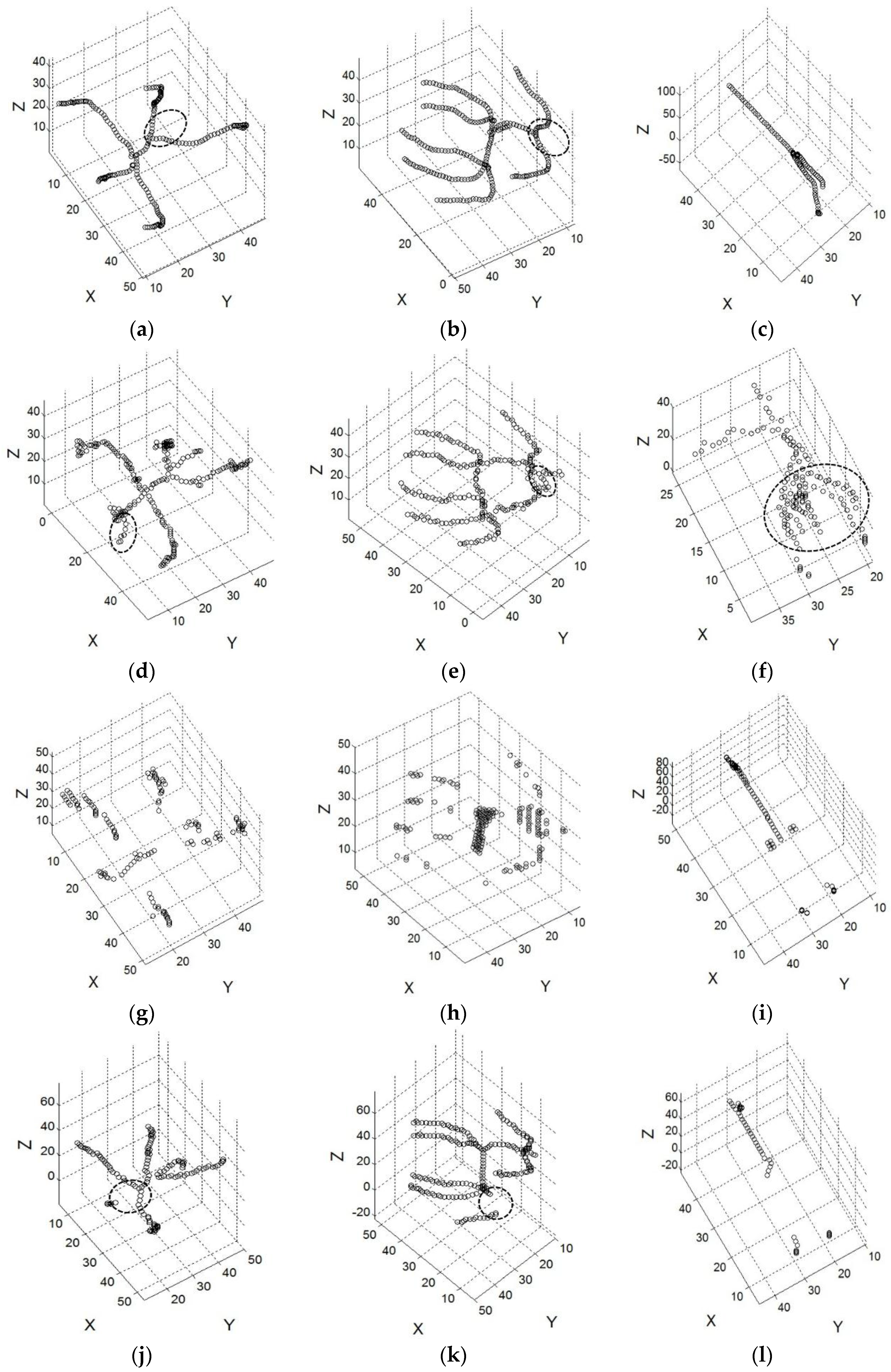
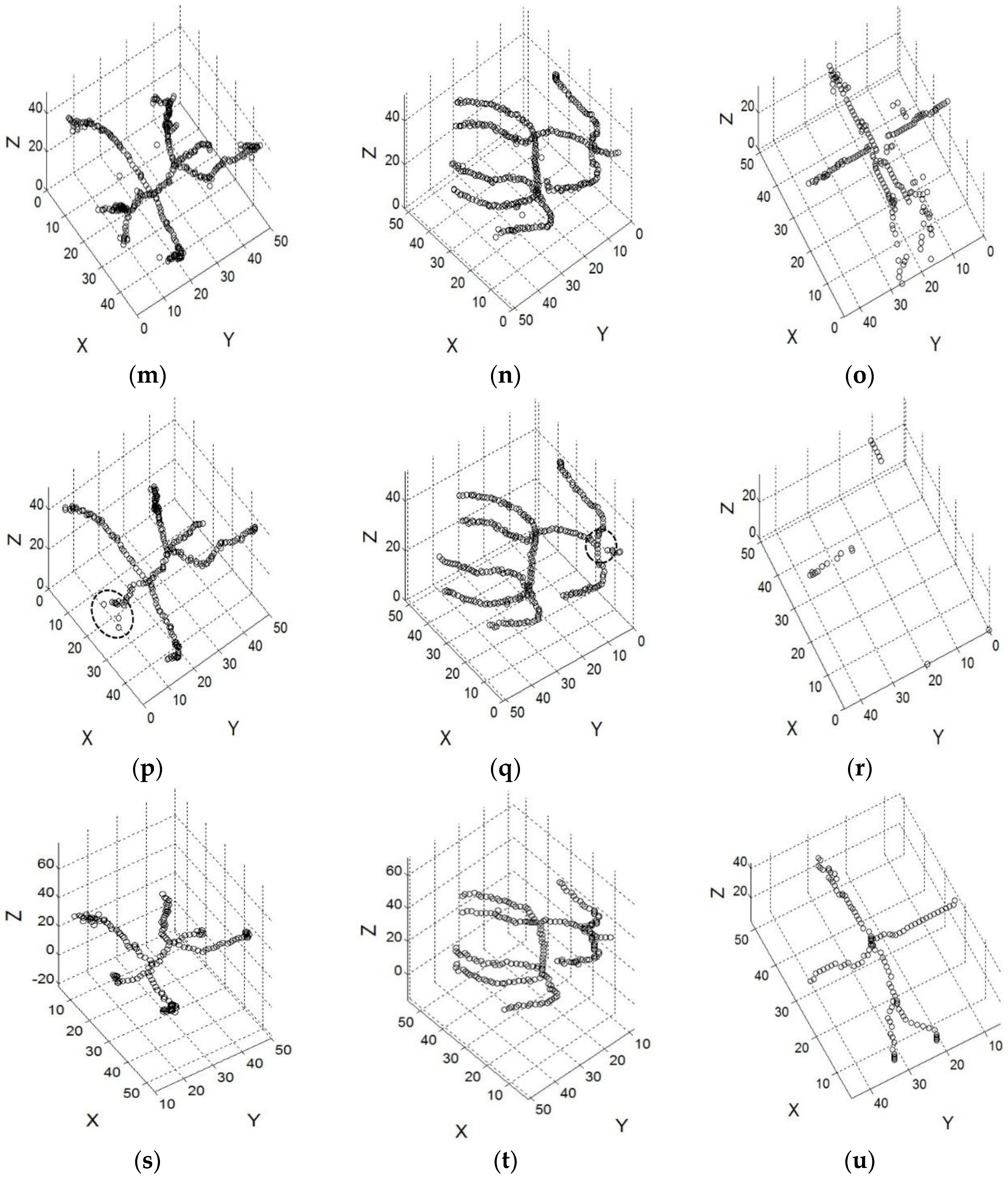
The skeletons extracted by the six algorithms are shown in Figure 12. Figure 12a–c shows the skeletons extracted by FMM. The skeletons of the armadillo’s tail, the centaur’s head and the manta ray model’s wings are not extracted. Figure 12d–f shows the skeletons extracted by MSA. The skeletons of the armadillo’s and the centaur’s heads contain spurious branches. Especially in Figure 12f, the skeleton of the manta ray model has many branches that are not essential. Figure 12g–i shows the skeletons extracted by MTTAC. Because too many voxels of the skeletons are removed, the skeletons are widely scattered. Figure 12j–l shows the skeletons extracted by FPT. The skeletons of the armadillo’s head and the centaur’s tail are disconnected, and those of the manta ray model’s wings are not extracted. Figure 12m–r shows the skeletons extracted by CCMP. We adjusted the MP score to extract a connected skeleton of the centaur. However, the skeleton contained some noises as shown in Figure 12n. With the same MP score, the extracted skeletons of the armadillo and the manta ray contained more noises as shown in Figure 12m,o. We also adjusted the MP score to extract a skeleton of the centaur without noise. However, the skeleton of the centaur’s head is disconnected as shown in Figure 12q. With the same MP score, the skeleton of the armadillo’s head is also disconnected as shown in Figure 12p. There was almost no skeleton extracted from the manta ray as shown in Figure 12r. Figure 12s–u show the skeletons extracted by the proposed algorithm. It extracts the skeletons of the manta ray model’s wings and does not extract spurious branches. The connectivity of the skeletons of the models are also preserved. To evaluate the robustness of the proposed method, we reduced the number of triangles of the models to 50% and scaled the sizes of the models to 50%. If the number of triangles is decreased, the smooth surface of the 3D model becomes rough. Thus, the generated voxels are also rough like adding noises. Scaling the size of the 3D model means that the volume of the 3D model is reduced. Figure 13 shows the skeletons extracted from the changed models. They are very similar to those of the original models, which means that the proposed method is robust to the change in the number of patch faces and of scaling sizes.

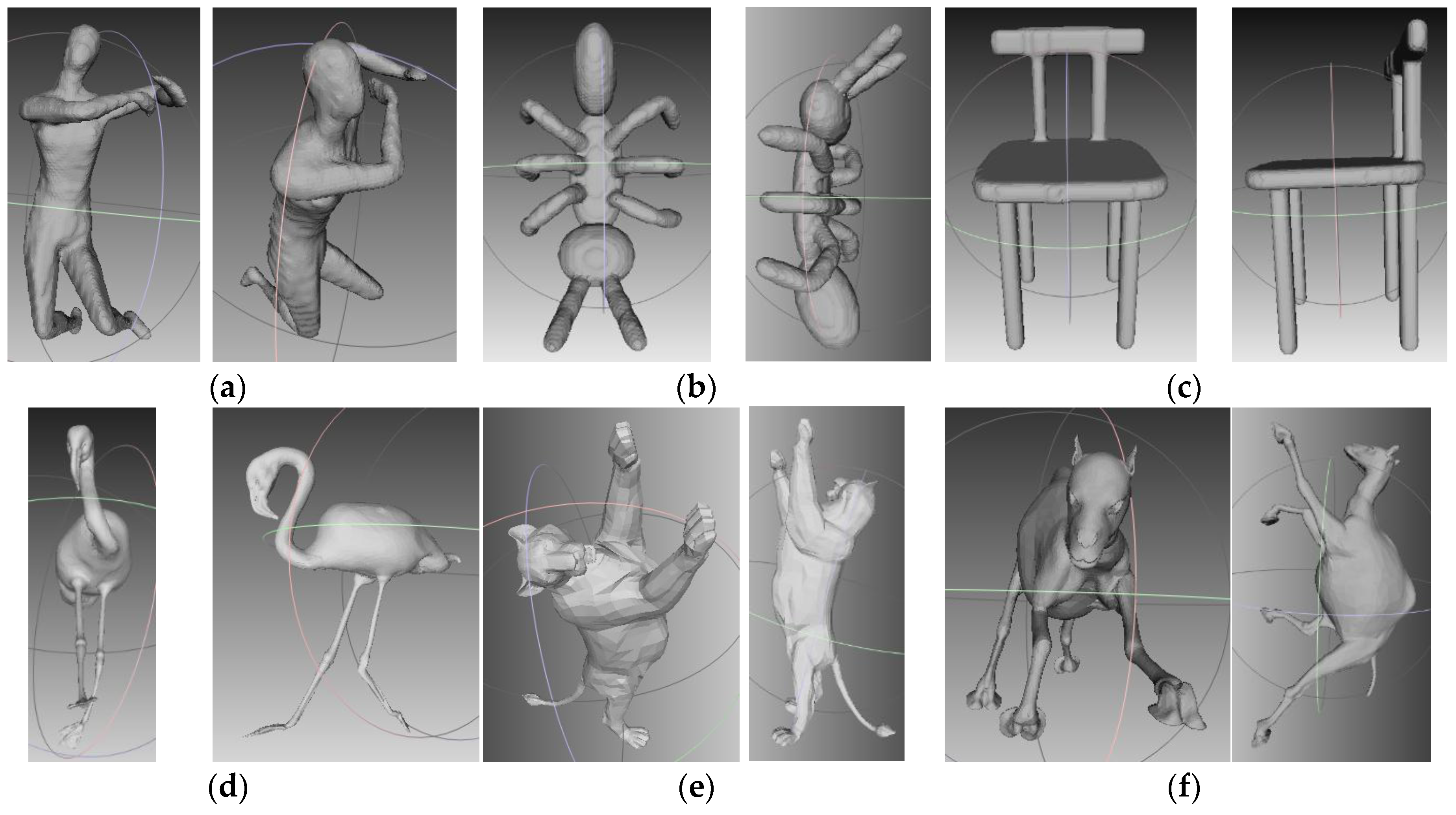
We also evaluated the proposed method with 10 models in the McGill 3D shape benchmark [30] and 7 models in the Sumner’s dataset [31]. Figure 14 shows six selected models: man, ant, chair, flamingo, lion, and camel. The first three of them were selected from the McGill 3D shape benchmark, and the remainder were selected from Sumner’s dataset. Figure 15 shows that most of the skeletons preserve connectivity, except for the flamingo. Because of the flamingo’s thin webbed feet, voxels cannot be generated uniformly inside the webbed feet during the voxelization process. Therefore, in the beginning, the voxels of the webbed feet were disconnected before the thinning procedure. It leads to the disconnection of the skeleton.

8. Conclusions

In this paper, we present a 3D skeletonization algorithm for 3D mesh models using a partial parallel 3D thinning algorithm and a 3D skeleton correcting algorithm. The partial parallel thinning algorithm assigns 62 symmetrical removing templates into two groups based on symmetry and thins the 3D model with the templates of each group in each thinning iteration. The skeleton correcting algorithm inspects the disconnected voxels in the skeleton and corrects them based on the six recovering templates and an additional criterion. The key advantage of this work is to extract a connected skeleton of each part of the 3D model simply and practically.

During the experiment, we evaluated the proposed algorithm with 117 models from three 3D model datasets. First, we compared the algorithm with five other skeletonization algorithms with 100 models in the SHREC 2015 benchmark. The comparison results of three representative models of animals and humans show that the proposed algorithm provides better connectivity and shows good performances. The evaluated results of robustness show that the algorithm is robust to the change in the number of triangles and of scaling sizes. We also evaluated the algorithm with 10 models in the McGill 3D shape benchmark and 7 models in the Sumner’s dataset. The overall experimental results show that the proposed algorithm can repair the disconnection and provide corrected skeletons. In future work, we will research error correcting of skeleton disconnection for the models with very small volumes and very thin webbed shapes, such as flamingo feet. We will also apply the algorithm to the identification of 3D models for preventing the copyrighted 3D models from being distributed illegally.