Article

Structural Performance of Composite Shear Walls under Compression

1
Key Laboratory of Urban Security and Disaster Engineering (Beijing University of Technology), Ministry of Education, Beijing 100124, China
2
School of Civil Engineering, Tangshan University, Tangshan 063000, China
3
Beijing Collaborative Innovation Center for Metropolitan Transportation, Beijing University of Technology, Beijing 100124, China
4
College of Civil and Architectural Engineering, North China University of Science and Technology, Tangshan 063000, China
*
Author to whom correspondence should be addressed.
Appl. Sci. 2017, 7(2), 162; https://doi.org/10.3390/app7020162
Submission received: 13 October 2016 / Revised: 23 January 2017 / Accepted: 4 February 2017 / Published: 9 February 2017
(This article belongs to the Special Issue Applications of Thin-Walled Structures)

Abstract

:
In order to research the effect of different layout forms of steel plate on the axial compression behavior of a steel plate-concrete composite shear wall, this paper presents the experimental results and analysis of the axial compression behavior of a composite shear wall, with different layout forms of steel plate. A total of three tests were carried out, composed of two composite walls with built-in steel plate, and one composite wall with two skins of steel plate. The gross dimensions of the three specimens were 1206 mm × 2006 mm × 300 mm. Experimental results show that the composite wall with two skins of steel plate has an optimal ability of elastic-plastic deformation, and the maximum axial compressive bearing capacity among the three specimens. Using the energy method, the critical local buckling stresses of steel plate were calculated, and compared with the yield stresses. According to different confined actions of concrete, concrete constitutive models were proposed, and the axial compressive strengths of confined concrete were calculated. Considering the local buckling of steel plate and confined concrete, the calculation formula of the axial compression of the composite wall was put forward, and the calculated results were in good agreement with the test results. Therefore, the different layout forms of steel plate have a great influence on its buckling, and on the concrete inhibition effect, which can affect the axial compressive bearing capacity of the composite wall.

1. Introduction

The composite shear wall with steel plate and concrete refers to a new type of shear wall structure, which is mainly used in super high-rise buildings, and missile-and blast-resistant walls. The composite shear wall has a broad prospect of application due to its high bearing capacities and the reduction in its thickness, especially at the strengthened bottom of the core tube in super high-rise buildings, which have a higher requirement for the cooperative performance between the steel plate and concrete. However, the local instability of steel plate may lead to poor cooperative performance, which has a great influence on the axial compression performance of composite walls. Some related research on the axial compressive performance of composite walls has been carried out in recent years. The axial compressive performance of composite walling, comprising two skins of profiled steel sheeting with an infill of concrete, was analyzed by Howard Wright [1,2]. Wright found a poor cooperative performance and a reduced axial compression capacity, due to the lack of a connection between the steel plate and concrete. Moreover, he reported that the axial compressive bearing capacity was affected by the local buckling of the steel plate and the eccentric cross-section of concrete, when different constructional measures between the steel plate and concrete were used to strengthen the cooperative performance. Md Azree Othuman Mydin [3] considered the buckling effect of steel plate on the axial compressive bearing capacity of a lightweight steel-foamed concrete-steel composite walling system, and presented a calculation formula for the axial compressive bearing capacity, using the concept of a steel plate buckling coefficient and an effective width, proposed by Uy [4,5]. The double-skin steel concrete composite shear wall with a "J" interlocking hook, was put forward by Zhenyu Huang [6]. Axial compression tests using 15 specimens were carried out and the calculation formula for the axial compression bearing capacity was put forward, considering the buckling influence of the steel plate. Xiaodan Fang [7] carried out axial compression experiments using asteel-tubehigh-strength concrete shear wall, for which a bearing capacity calculation formula was established. The axial compression tests on the local stability of a composite wall with two skins of steel plate, were studied by Youjia Zhang [8], for which the theoretical formula for the elastic buckling of steel plate was derived. The constitutive model of the core concrete in the steel plate concrete composite shear wall with constraint bars, was theoretically analyzed by Hongliang Liu [9].
However, previous research has paid little attention to the arrangement of steel plate within composite walling systems, which has a great influence on the cooperative performance between the steel plate and concrete. Therefore, axial compression experiments with different layout forms of steel plate were carried out in the subsequent study. This paper proposed a calculation equation for the axial compressive bearing capacity, considering local buckling of steel plate and the increase in the axial compressive strength of confined concrete. The calculated results were in good agreement with the test results.

2. Experiments

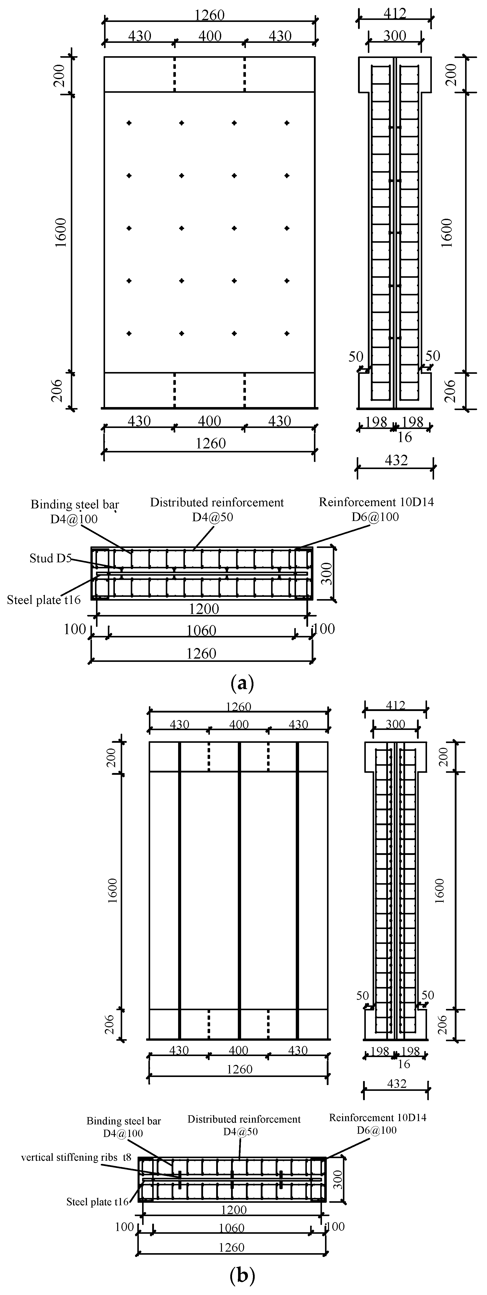
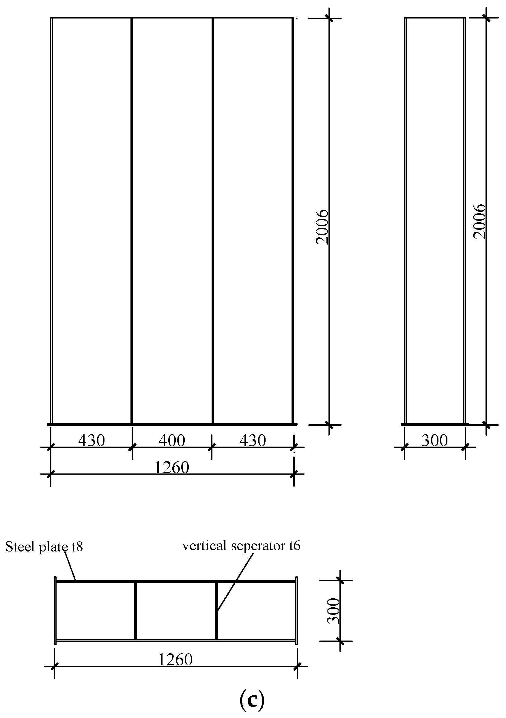
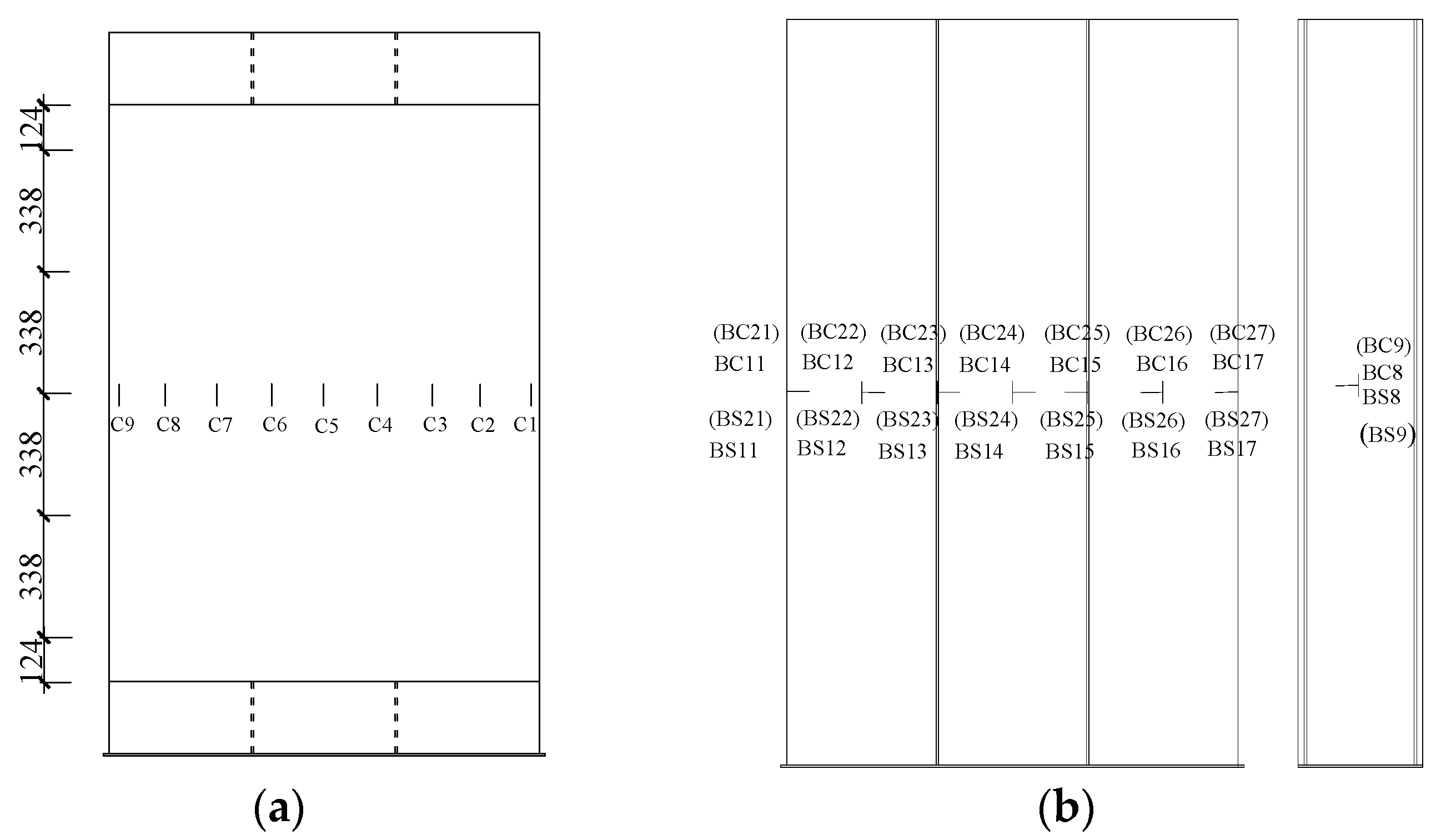
2.1. Geometrical Descriptions of Specimen

The gross dimensions of the three test specimens were 2006 mm high × 1260 mm wide × 300 mm. The steel plates of 16 mm thickness were arranged inside the composite shear wall of specimens HGW-1 and HGW-2. The difference between the two specimens was the construction measure between the steel plate and concrete. The steel plate of specimen HGW-1 was welded with studs which had a diameter of 5 mm, length-diameter ratio of 5, and spacing of 300 mm. The six vertical stiffening ribs with a width of 50 mm and thickness of 8 mm, were set on both sides of the steel plate of the HGW-2 specimen. For specimen HGW-3, steel plates of 8 mm thickness were arranged on the outer sides of the composite wall, where two skins of steel plate were connected by vertical separators, which had a thickness of 6 mm, and an interval of 400 mm. Figure 1 shows the section sizes and details of the three test specimens.

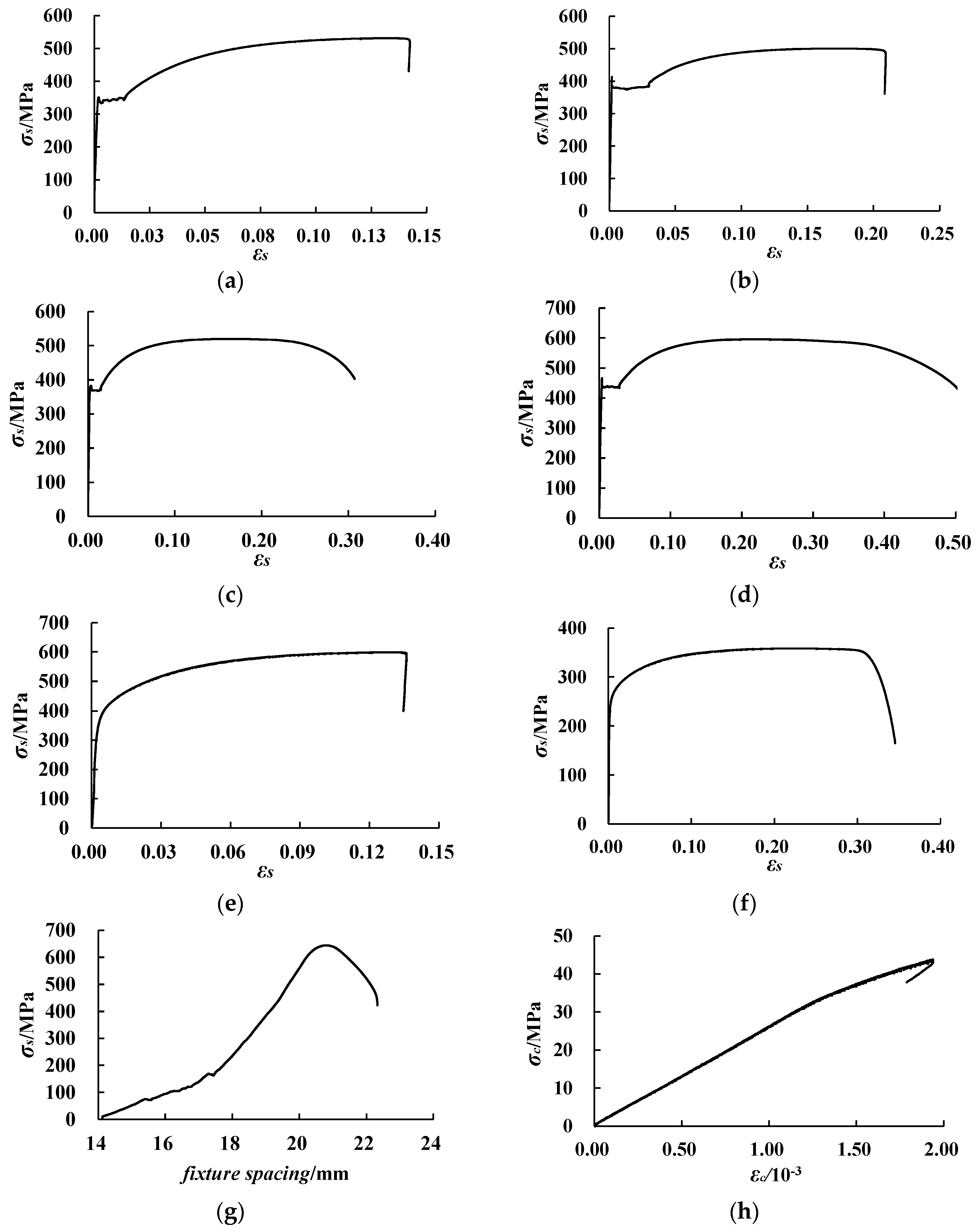
2.2. Material Properties

The concrete design strength grade of C55 was adopted in the initial stage of the design. Three specimens were cast with the same batch of concrete, from which three concrete cubes of 150 mm, and three concrete cylinders of 150 mm × 150 mm × 300 mm, were obtained. After 28 days of casting, the concrete cubes and cylinders were tested in the compression machine. The average value of the cube compressive strength fcu,m was 56.71 MPa. The axial compressive strength fck, was taken as 0.76 fcu,m, with a value of 43.1 MPa. An elastic modulus of 2.61 × 10⁴ MPa was obtained from the cylinder tests.
Tensile tests of the steel plate, studs, steel bar, and lead wire of the three groups, were conducted to obtain the yield strength fy, tensile strength fu, elongation percentage δ, and elastic modulus Es. Table 1 shows the test results for the mechanical properties of the steel materials, respectively. According to the results of these mechanical tests, the yield strain of the steel plate with a 16 mm thickness was 1616 × 10−6 and that with an 8 mm thickness was 1799 × 10−6, by calculation. The representative stress-strain material curves were obtained from the tensile tests of steel materials, as can be seen in Figure 2a–g. The concrete stress-strain material curve in Figure 2h only illustrates the concrete characteristics of the elastic stage, as it was produced from the elastic modulus tests, in which the peak load and descending segment were not measured.

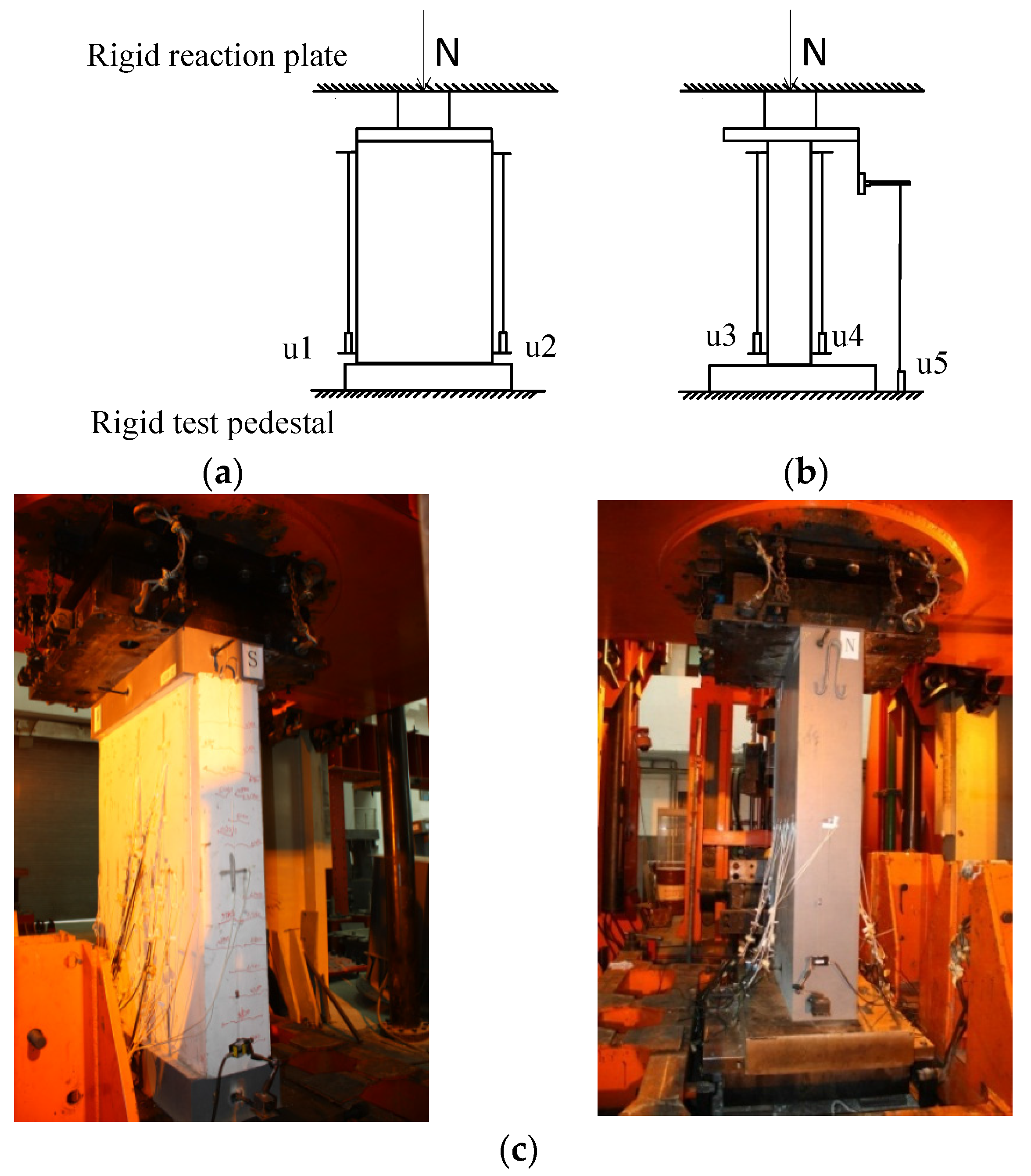
2.3. Loading and Measuring Scheme

The experiments were carried out on a pressure testing machine, with a maximum bearing capacity of 40,000 kN, which belongs to a multi-function electro hydraulic servo loading test system, equipped with a one-way ball hinge support at the loading end. The loading device is shown in Figure 2 and the center of the loading support coincides with the center of the section combination. Firstly, each test specimen was pre-loaded with 1500 kN for five minutes, to check whether the test points were normal or not, before being unloaded to zero. Secondly, a force control loading mode was adopted in the experiments, which included multi-stage loading with an 1800 kN increment before 20,000 kN, and loading with a 900 kN increment after 20,000 kN. The peak load of every stage was maintained for two minutes, in order to observe concrete cracks or local buckling of the steel plate. Thirdly, a displacement control loading mode of 2 mm was made after the ultimate load.
The data recorded for the load, displacement, and strain, were obtained in real-time by an IMP data acquisition system. Four wire-type displacement meters were arranged around the test specimen, to measure the vertical deformation. Another wire-type displacement meter monitored the deformation between the rigid bearing surface of the upper axial compression actuator, and the rigid test pedestal of the loading system. The arrangements of the five displacement meters are shown in Figure 3.
The strain gauges of the concrete and steel plates were arranged at the mid-height of every specimen, as shown in Figure 4, including the vertical and horizontal layout, for which the strain gauges of the steel plate are in the same position as that of the concrete, for specimens HGW-1 and HGW-2.

3. Experimental Results

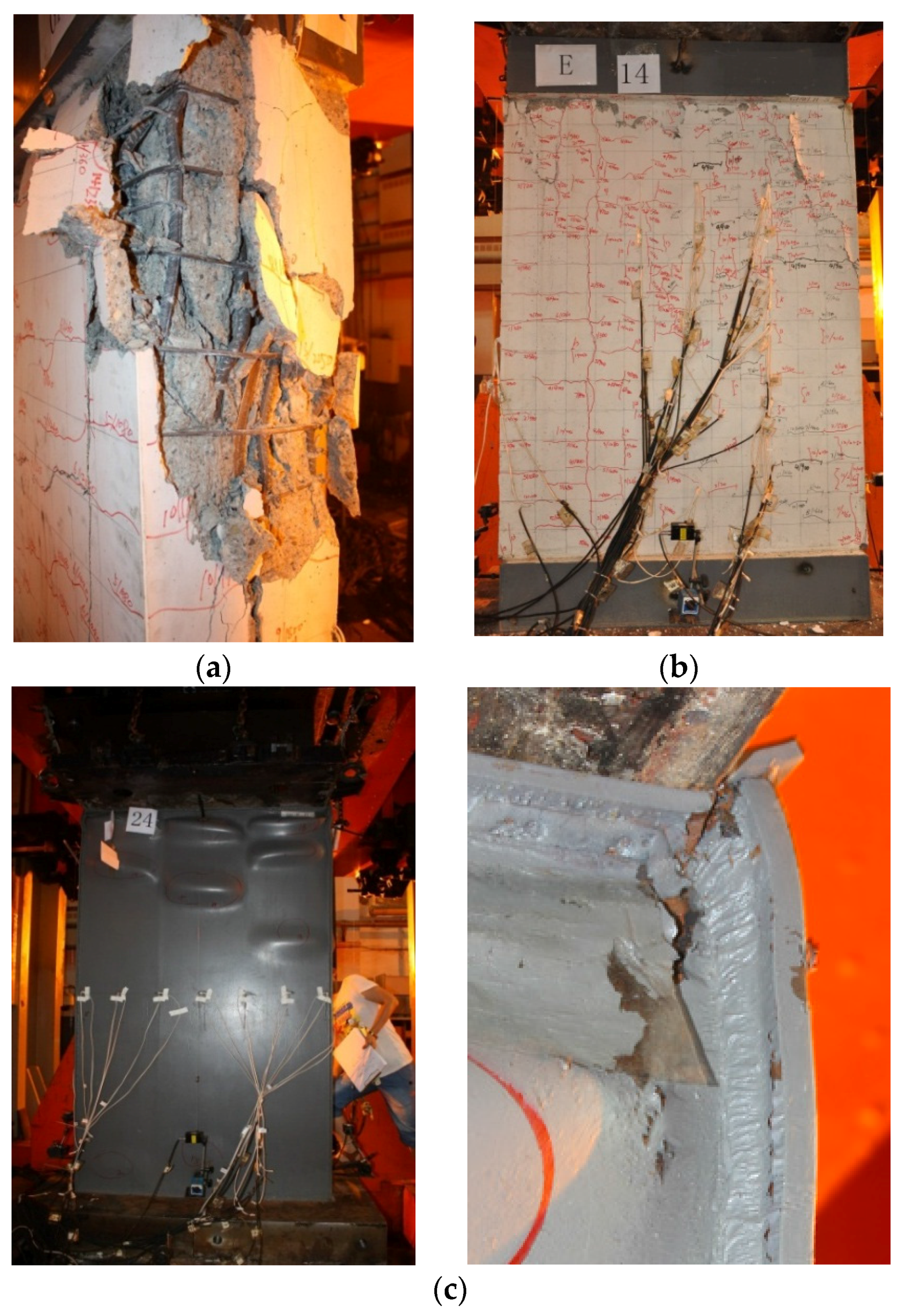
3.1. Experimental Phenomena and Failure Modes

For specimens HGW-1 and HGW-2, vertical cracks first appeared at the upper east side with 3600 kN loading and 5400 kN loading, respectively. With the increase in the load step, more vertical cracks appeared, and previous cracks became wider, with a maximum width of 3 mm and 1 mm, respectively. For specimen HGW-1, the concrete collapsed suddenly at the upper east side and upper north side, when the ultimate load had been reached, and the steel plate was bent at the upper 400 mm height, exposing the horizontal distribution reinforcement. For specimen HGW-2, apparent damage phenomena did not appear at the ultimate load, and the concrete at the eastern side cracked after having been twice loaded with displacement controlling. In contrast to specimen HGW-1, the structural integrity of specimen HGW-2 behaved better, and the brittle performance improved greatly.
For specimen HGW-3, shear slip lines of 45 degrees appeared at the crossing of the steel plate and vertical separators, of the upper 800 mm height. With the increase of the load step, the number of shear slip lines became higher, and they also became denser. The local buckling of the steel plate appeared and winkled at 19,800 kN loading, and the local buckling gradually increased until its maximum thickness reached 8mm at the ultimate load, at which point the weld lines at the top of the steel plate were torn. The region of local buckling between the vertical separators developed after loading ten lots of the displacement controlling, and the maximum bulging drum reached 85 mm. The test specimen maintained a bearing capacity, of about 50% of the ultimate load, and showcased a good ductility performance. Figure 5 shows the failure modes of each specimen.

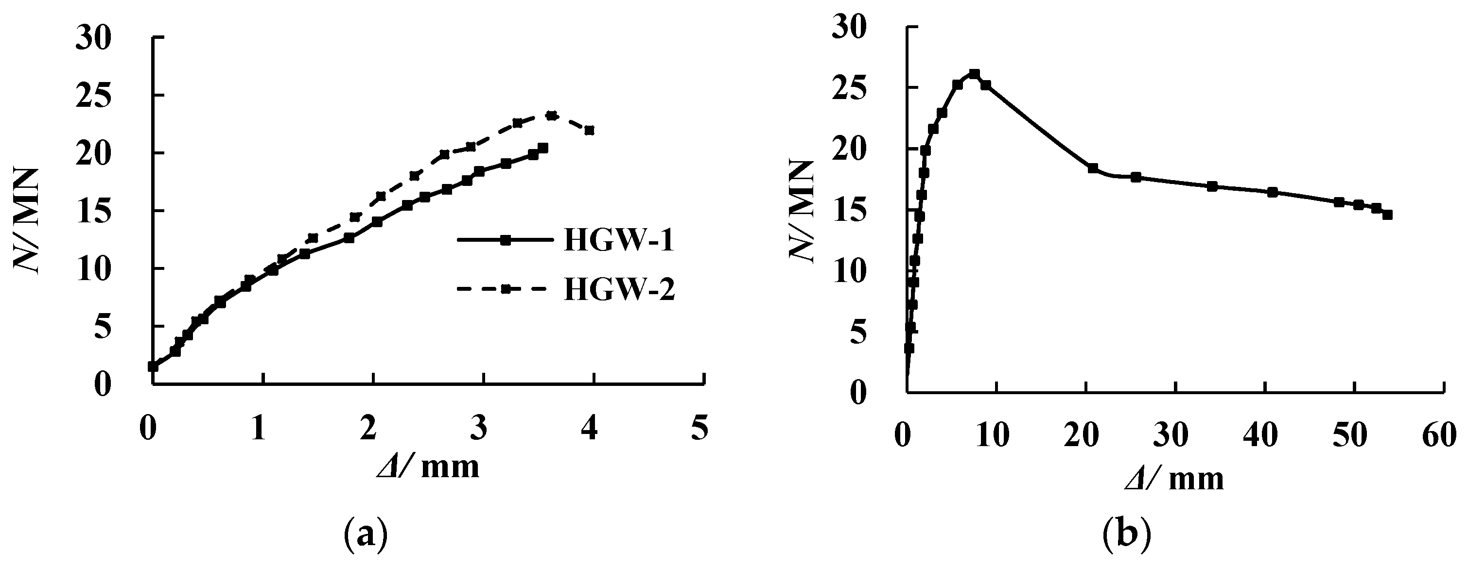
3.2. Force-Displacement Curves

Figure 6 shows the relationship curves of the axial force versus the axial displacement, which was obtained by recording the average value of four wire-type displacement meters on each side. Since the concrete was rapidly crushed, and the concrete inhibition effect was weakened, specimen HGW-1 was damaged at the ultimate load. However, since the vertical stiffening ribs on both sides of the steel plate constrain the development of a single wave outside of the steel plate, specimen HGW-2 continued to bear loads, even after the ultimate load. The curve of HGW-3 was gentler, mainly because the two skins of the steel plate were able to effectively constrain the transverse deformation of the inner concrete.
Table 2 lists the load values and displacement values of the three test specimens at every stage. For specimen HGW-3, the crack load cannot be obtained, due to the in-filled concrete, and the failure load was assumed to be 15% of the ultimate load, according to the literature [10]. Compared to specimen HGW-1, the axial compressive bearing capacity of specimen HGW-2 increased by 13.59%, and the axial deformation increased by 2.32%, mainly because the stiffening ribs delayed the compressive strain development of the concrete, and improved the cooperative performance between the steel plate and concrete. In contrast to specimen HGW-1, the axial compressive bearing capacity of specimen HGW-3 increased by 28.21%, and the axial deformation increased by 112.25%, chiefly because the outer steel plate kept the concrete in a state of multi-axial compression, and the inner vertical separators played the role of a web. For specimen HGW-3, the corresponding displacement at the failure load was 1.76 times higher than that at the ultimate load, and 6.09 times higher than that at the yield load, which indicated that the composite shear wall with two skins of steel plate, demonstrated a good elastic-plastic deformation performance.

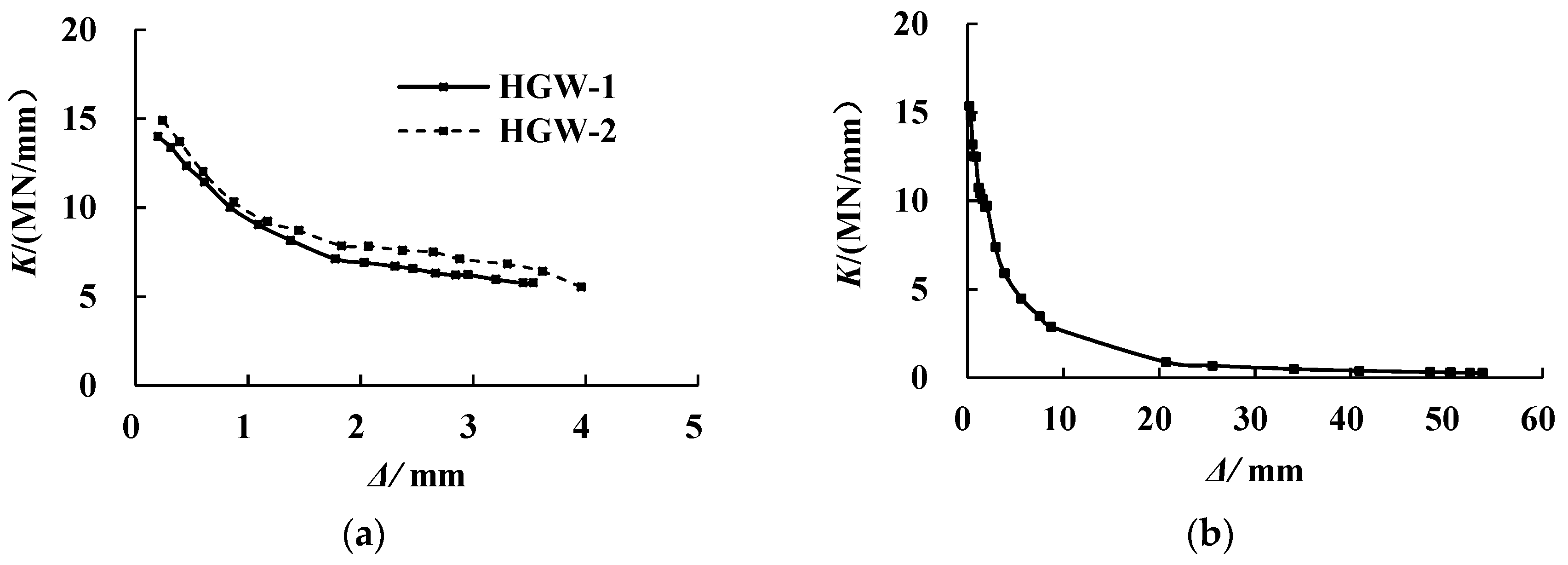
3.3. Degradation of Axial Rigidity
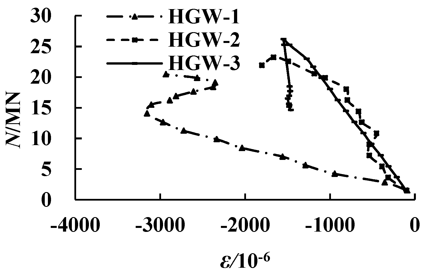
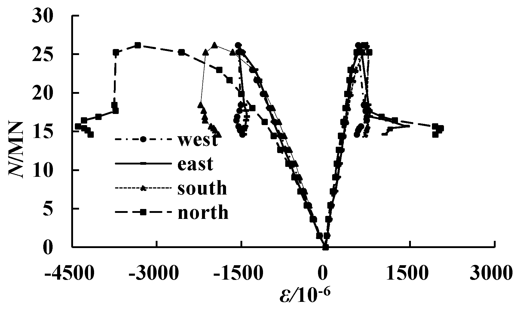
The axial stiffness of the experiments can be calculated as follows [8]:
K i = N i / Δ i
In which, Ni and Δi denote the peak load and corresponding displacement under every loading, respectively, i denotes the step of loading, and Ki denotes the axial stiffness. The initial axial stiffnesses K1 of the three specimens, utilizing Equation (1), were 14,005 kN/mm, 14,980 kN/mm, and 15,372 kN/mm, respectively.
The calculated formula for the initial axial stiffness is defined as follows [8]:
K c a l = E s A s + E c A c
In which Es and Ec denote the elastic modulus of the steel plate and concrete, respectively, and As and Ac denote the cross-sectional area of the steel plate and concrete, respectively. The calculated values of the three specimens are 13,511 kN/mm, 14,021 kN/mm, and 14,352 kN/mm, respectively, which are lower than the test values of 3.66%, 5.49%, and 7.11%, mainly because the concrete inhibition effect is not considered in the calculation of the elastic modulus.
Figure 7 shows the stiffness degradation curves of the axial stiffness versus the axial displacement. For specimens HGW-1 and HGW-2, the corresponding stiffness of the failure load, declined by 58.8% and 62.9%, respectively, when compared to the initial stiffness. For specimen HGW-3, the stiffness of the yield load declined by 51.9%, the stiffness of the ultimate load decreased by 77.3%, and the stiffness of the failure load declined by 99.4%. Therefore, it is revealed that the stiffness degradation of specimen HGW-3 is faster than specimens HGW-1 and HGW-2 at every stage, and is sufficient during the whole progress.

3.4. Strains

Figure 8 describes the curves of the axial load versus the steel plate strain, which are the average values of the mid-height vertical strains, with the negative value corresponding to the compression. From test experiments, it was shown that the steel plate of specimen HGW-1 yielded at 10.81 MN load, while the steel plate of specimens HGW-2 and HGW-3 yielded at the ultimate load. Therefore, the yield strength of the steel plate can be used in the subsequently calculated formula of the axial compressive bearing capacity. As shown in Figure 7, the strain of specimen HGW-1 increased more rapidly than specimen HGW-2, mainly because the vertical stiffening ribs on both sides increased the rigidity of the steel plate, and the horizontal distribution of the steel bar through the holes of the ribs strengthened the cooperative performance of the steel plate and concrete.
Figure 9 shows the changing-rule curves of the vertical strain and circumferential strain of specimen HGW-3, which were the average value of each side. The vertical strain was expressed by the compressive strain, with a negative value on the left side of Figure 9, while the circumferential strain corresponded to the tension strain, with a positive value on the right side of Figure 9. It was observed that four circumferential strain curves were basically coincident, which revealed that the deformations of each side were uniform. During the whole loading process, the increase rate of the vertical strain was greater than that of the circumferential strain before the ultimate load, which indicated that vertical deformation became the major part in this stage. The vertical strain of the steel plate marginally reduced after the ultimate load, while the circumferential strain gradually increased, chiefly because the constraint effect of the steel plate on the concrete was no longer increased after the yielding of the steel plate, so circumferential deformation of the concrete and circumferential tension stress of the steel plate could rapidly increase.

4. Calculation for Axial Compressive Bearing Capacity

From the above analysis of the composite wall, the actions of the steel plate and concrete are apparently different among the three specimens, due to the various layout forms of the steel plate, which directly affects the cooperative performance of the steel plate and concrete, as well as the axial compressive bearing capacity. Therefore, the bearing capacity of the steel plate and the concrete inhibition effect will be analyzed under different conditions.

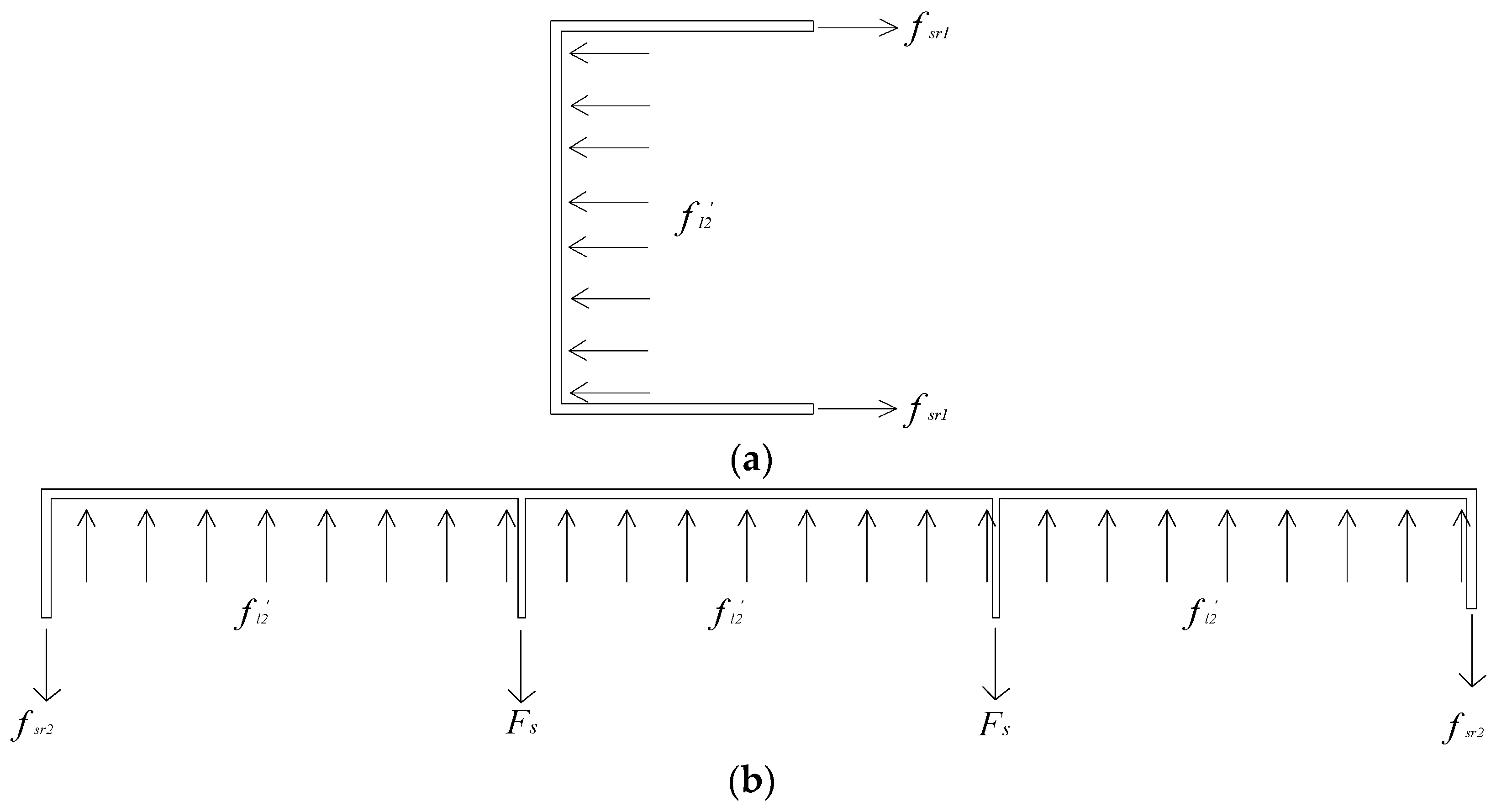
4.1. Steel Plate Resistance

Figure 10 shows a rectangle plate with a × b, uniform pressure Nx, per unit length in x direction, in which four sides are regarded as simply supported. It can be assumed that the supporting points of the steel plate can move freely in the plane, due to the fact that steel plate bends slightly under uniform compression. The critical local buckling load of the steel plate was calculated using the energy method, without considering the initial defect of the steel, in which the total potential energy included the strain energy of the steel plate, and the potential energy of the external force.

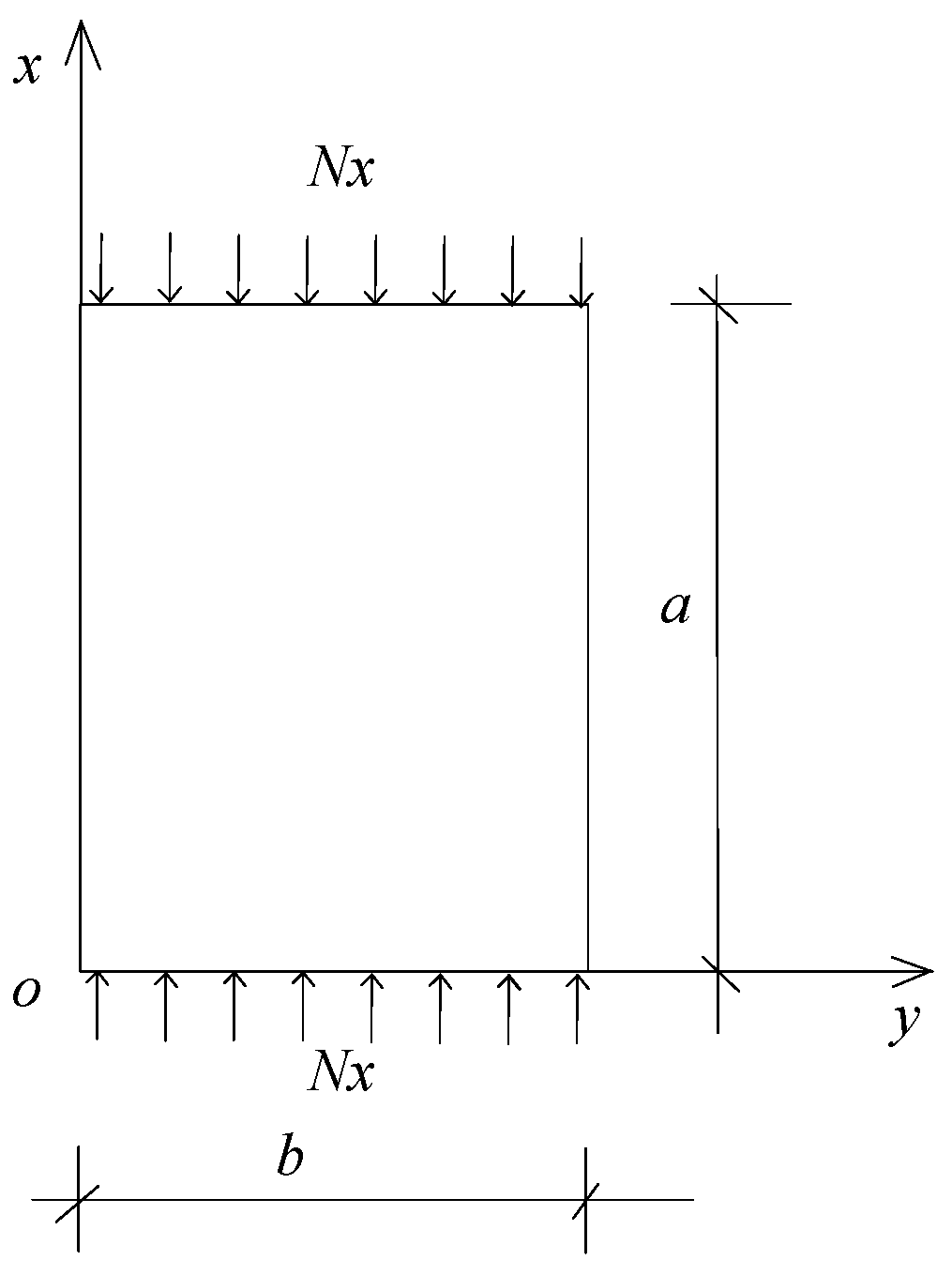
4.1.1. Local Buckling Analysis of Unstiffened Steel Plate

Since the steel plate of specimen HGW-1 was surrounded by four neighboring studs, and the steel plate of specimen HGW-3 was divided into three narrow plate-strips by vertical separators, the simple support on four edges can be applied without a rotation constraint.
The strain energy of the steel plate under slightly bending can be established using the following equation [11]:
U = 1 2 0 a 0 b ( M x 2 w x 2 + M y 2 w y 2 + 2 M x y 2 w x y ) d x d y = D 2 0 a 0 b { ( 2 w x 2 + 2 w y 2 ) 2 2 ( 1 υ ) [ 2 w x 2 × 2 w y 2 ( 2 w x y ) 2 ] } d x d y
In which ν denotes the Poisson ratio; ω denotes the plane deflection at any point; Mx, My denote the bending moment caused by plate bending; Mxy denotes the torque caused by plate bending; D denotes the bending rigidity of the steel plate, considering the Poisson ratio presented in the following equation:
D = E t 1 3 12 ( 1 υ 2 )
In which E denotes the elastic modulus, and t1 denotes the thickness of steel plate.
The potential energy of the external force can be shown in the following equation, from the straight state of the steel plate, to the bending state [11]:
V = 1 2 0 a 0 b N x ( w x ) 2 d x d y
According to the above equations, the total potential energy was the sum of the strain energy and the potential energy:
Π = U + V = D 2 0 a 0 b { ( 2 w x 2 + 2 w y 2 ) 2 2 ( 1 υ ) [ 2 w x 2 × 2 w y 2 ( 2 w x y ) 2 ] } d x d y 1 2 0 a 0 b N x ( w x ) 2 d x d y
Based on the small deflection theory, the equation for the critical local buckling was derived using the Rayleigh-Ritz method [11], in which a double trigonometric series was assumed as the bending surface function of the steel plate:
w = m = 1 n = 1 a m n sin m π x a sin n π y b
where m, n reflect the half wave number along the x, y direction, after bending of the steel plate. Furthermore, Equation (7) conforms to the geometric boundary condition: w = 0 when x = 0 and x = a; w = 0 when y = 0 and y = b. So, Equation (7) was incorporated into Equation (6), and the following equation was obtained, after a series of integration:
Π = π 4 a b D 8 m = 1 n = 1 a m n 2 ( m 2 a 2 + n 2 b 2 ) 2 π 2 b N x 8 a m = 1 n = 1 a m n 2 m 2
According to the principle of stationary potential energy, a group of linear algebraic equations, such as Π a 11 = 0 , Π a 12 = 0 , Π a m n = 0 were established, and the critical buckling equation was determined using the conditions of a non-zero solution:
N x = π 2 D b 2 ( m b a + n 2 a m b ) 2
Considering that the uniform pressure plate usually produced one half-wave in the transverse direction [12] (i.e., n = 1), m = a/b can be obtained from N x m = 0 with a continuous variable of m. The critical buckling local load (i.e., the minimum value of Nx) and the critical buckling stress were obtained as follows:
N x = 4 π 2 D b 2
σ c r = 4 π 2 D b 2 t

4.1.2. Local Buckling Analysis of Stiffened Steel Plate

For the steel plate with stiffening ribs, the stiffening coefficient κ represents the effect of axial rigidity and torsional rigidity on the improvement of the local strength, which is defined as the following equation [9]:
κ = A 1 / A
where A1 is the cross-sectional area of the stiffening ribs, and A is the cross-sectional area of the steel plate.
Since the stiffening coefficient κ of specimen HGW-2 is 0.125, the axial rigidity and torsional rigidity of specimen HGW-2 are neglected, without considering the initial inflect of the steel plate [13]. Besides, the boundary condition of the steel plate with stiffening ribs was assumed to be simply supported on four edges, the critical buckling load was calculated by the energy method, and the deflection surface function was adopted by Equation (7). For the stiffening ribs, the strain energy and the potential energy of the external force can be calculated using the following equations [11]:
U = E I 0 a [ ( 2 w x 2 ) 2 y = b / 4 + ( 2 w x 2 ) 2 y = b / 2 + ( 2 w x 2 ) 2 y = 3 b / 4 ] d x
V = A N x 0 a [ ( 2 w x 2 ) 2 y = b / 4 + ( 2 w x 2 ) 2 y = b / 2 + ( 2 w x 2 ) 2 y = 3 b / 4 ] d x
where A and I denote the cross-sectional area and the inertia moment of one rib, respectively.
The total potential energy of the stiffening ribs was the sum of the strain energy and the potential energy of the external force, which was obtained after Equation (7) had been incorporated into Equation (15), with a series of integration:
Π = U + V = ( E I A N x ) 0 a [ ( 2 w x 2 ) 2 y = b / 4 + ( 2 w x 2 ) 2 y = b / 2 + ( 2 w x 2 ) 2 y = 3 b / 4 ] d x
Π = ( E I A N x ) π 4 a m = 1 n = 1 a m n 2 m 4
The total potential energy of the walling system is the sum of the two steel materials, including the steel plate and stiffening ribs. The potential energies of the stiffening ribs and steel plate should be superimposed in the calculation of the total potential energy, presenting the potential energy of the external force. Therefore, the following equation can be obtained through the superposition of Equations (8) and (16):
Π = π 4 a b D 8 m = 1 n = 1 a m n 2 ( m 2 a 2 + n 2 b 2 ) 2 π 2 b N x 8 a m = 1 n = 1 a m n 2 m 2 + ( E I A N x ) π 4 a m = 1 n = 1 a m n 2 m 4
In view of the single half-wave of the uniform pressure plate in the transverse direction [12] (i.e., n = 1), supposed m = 1 and Π a 11 = 0 were established, the coefficient determinant was viewed as zero, and the critical local buckling stress of the steel plate with the stiffening ribs was obtained.
N x = 8 a b + 8 A π 2 [ π 2 D ( a 2 + b 2 ) 2 a 2 b 3 + E I π 2 ]
σ c r = 8 a ( b + 8 A π 2 ) t [ π 2 D ( a 2 + b 2 ) 2 a 2 b 3 + E I π 2 ]

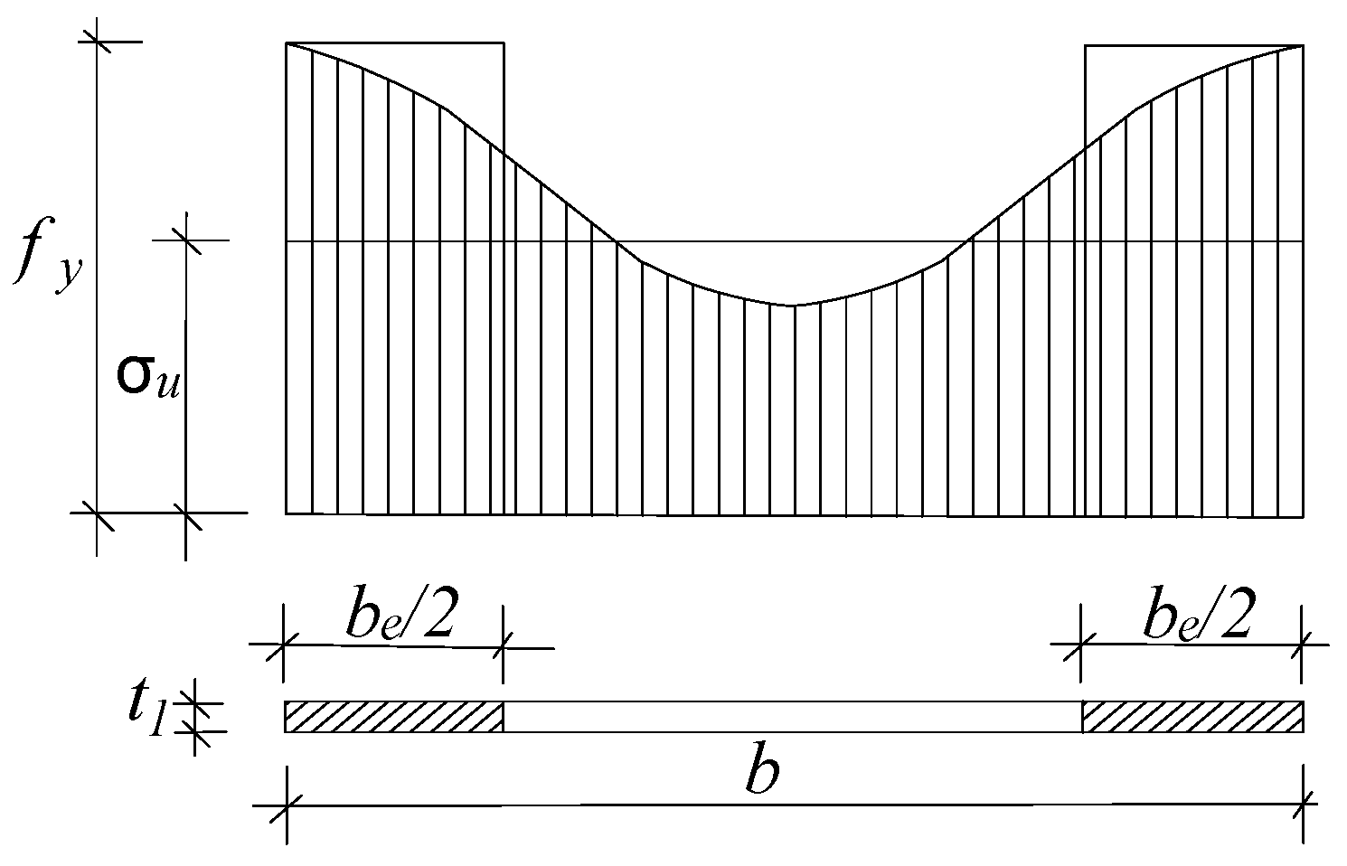
4.1.3. Effect of Local Buckling on Bearing Capacity

The critical local buckling stresses of specimen HGW-1 and HGW-3 were calculated using Equation (11), and the stress of specimen HGW-2 was calculated using Equation (19). The calculated values are shown in Table 3. For specimen HGW-1, the calculated buckling stress is smaller than the yield stress, but the buckling of the steel plate in the test is later than the steel yield, mainly because the concrete plays a role in the inhibition of the out-of-plane deformation of the steel plate. Until the concrete reaches the ultimate compressive strain at the ultimate load, the concrete inhibition effect on the steel plate decreases rapidly, and the buckling of the steel plate takes place immediately. For specimen HGW-2, owing to the concrete inhibition effect on the steel plate, the actual local buckling stress is far higher than the calculated buckling stress, which was originally larger than the yield stress, so the test buckling stress value does not appear in Table 3. Therefore, since the buckling is later than the yield for specimens HGW-1 and HGW-2, the effect of local buckling on the bearing capacity is unthinkable in the calculation of the axial compressive bearing capacity.
For specimen HGW-3, the calculated buckling stress is in good agreement with the test buckling stress shown in Table 3, and both buckling stresses are less than the yield stress, which means that local buckling occurs earlier than the yield of the steel plate. Due to uniform compression, the steel plate bends slightly after buckling, and the deflection in the central section is greater than that at the two edges, and the flexural shortening in the central section outweighs that at the two edges, which means that the stress redistribution occurs with greater stress at the two edges, and less stress in the central section. After local buckling of the steel plate occurs, the stress in the central section no longer increases, and the stress at the two edges continues to increase, until the yielding of the steel plate. So, the evaluation criterion for whether the steel plate reaches the ultimate load, is whether the plate edge yields or not. As shown in Figure 11, the plate stresses in the range of approximately be/2 at the two edges, only reach yield strength fy, when the effective width is introduced, in order to present an effective action of the steel plate at the ultimate load. According to Chen Shaofan [12], the ratio of the effective width to width b, can be calculated by the following equation:
b e b = σ c r f y [ 1 0.22 σ c r f y ]
where be is the effective width, b is the actual width, and σu is the average stress in the limit state.
The buckling influence coefficient of the steel plate η is defined as the ratio of effective width be to width b, and is introduced to the axial compressive bearing capacity formula of the steel plate.
N s = b e t 1 f y = η b t 1 f y
For specimen HGW-3, the calculated η value is 0.719, shown in Table 3.

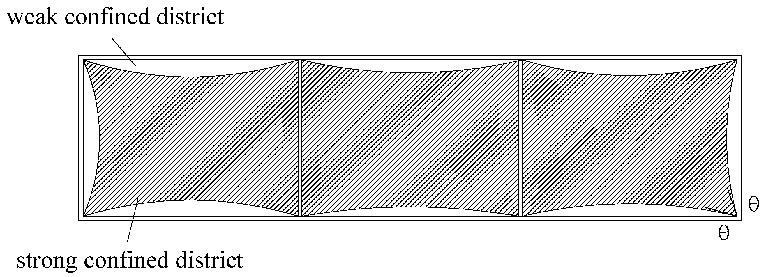
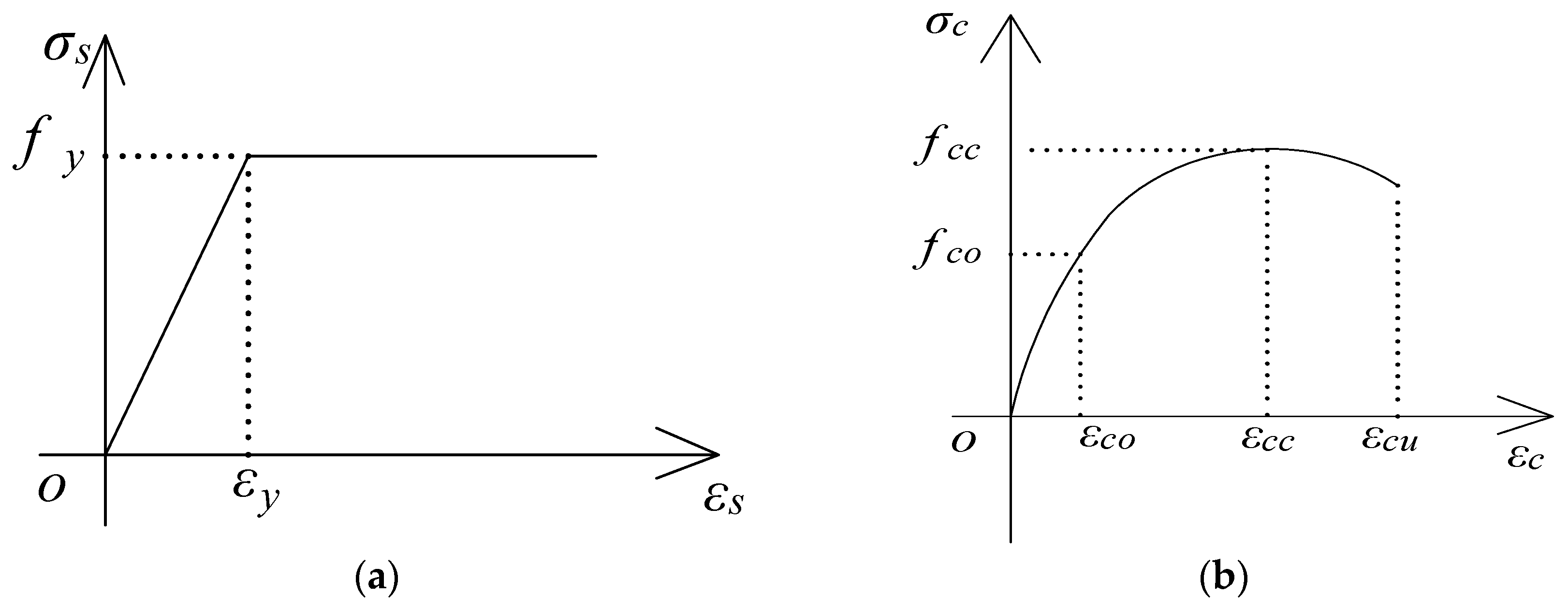
4.2. Strength of Concrete

4.2.1. Composite Wall with Two Skins of Steel Plate

For the two skins of the composite wall, the external steel plate has the same effect of longitudinal reinforcements and stirrups, and the internal vertical separator can inhibit the deformation of the walling system. The force mechanism of the core concrete inside the steel plate is similar to stirrup-confined concrete, so the Mander [14] method can be referenced in the following analysis of the concrete constitutive model, and parameter r was determined by [14].
σ c = f cc x r r 1 + x r ( 0 < ε < ε c u )
x = ε / ε c c
ε c c = ε c o [ 1 + 5 ( f c c f c o 1 ) ]
r = 145 × 0 . 4 × 10 3 f c o + 1 . 0
where σc is the compressive stress of the concrete, fcc is the compressive strength of the confined concrete; ε is the compressive strain of the concrete; εcc is the corresponding compressive strain of the confined concrete; fco is the axial compressive strength of the unrestrained concrete.
Figure 12 shows two force-separating bodies along the directions of the long side and short side, which includes the stress conditions and distribution. fl1′, fl2′ denote the transverse compressive stress of the steel plate along the two directions. fsr1, fsr2 denote the circumferential tensile stresses of the steel plate along the two directions, which are regarded as uniformly distributed because of the relatively thin plate-wall. Fs denotes the circumferential tensile stress of the internal vertical separator, which can be calculated by Hooke’s law, since the separator yielded at the ultimate load by test strain data.
Considering the establishing convenience of the force balanced equation, the transverse compressive stress of the steel plate is assumed to be of uniform distribution. In fact, the bending rigidity of the steel plate at the corner is larger than that in the middle, and the inhibition effect of the steel plate on the concrete is variable. Therefore, the concrete parts are divided into a strong confined district and a weak confined district, which may refer to the calculation method used in the literature [15]. Figure 13 shows a sketch of the confined concrete district, in which the confinement curve is regarded as a two-order parabola with θ = 12° [15]. In order to describe the uneven distribution of the transverse compressive stress of the steel plate along the two directions, the effective constraint coefficient Ke was introduced, in order to present the reduction of the compressive stress, and the formulae were deduced as follows:
f l 1 = f l 1 ' K e
f l 2 = f l 2 ' K e
K e = A e A e + A f
where Ae denotes an area of strong confined district, Af denotes an area of weak confined district, and fl1, fl2 denote the effective transverse compressive stress of the steel plate along the directions of the long side and short side.
The strain of the steel plate increased gradually, with the increasing of the vertical bearing-load, until the steel plate and vertical separator reached the yield strength. At this point, the core concrete began to expand, and the transverse deformation of the concrete and the circumferential tensile strain of the steel plate increased rapidly. The steel plate was in a state of three-dimension stresses, including vertical compressive stress, circumferential tensile stress, and radial compressive stress. However, the radial compressive stress was small, due to the thin wall of the steel plate with b/t ≥ 20, and is regarded as approximately zero [13]. So, the steel plate is only subjected to two dimension stresses, including axial compression and circumferential tension, and the steel plate is regarded as ideal elastic-plastic material. Therefore, the steel plate conforms to the yield criterion of Von Mises, when the steel plate yields as shown in the following equations:
f a 1 2 f a 1 f s r 1 + f s r 1 2 = f y 2
f a 2 2 f a 2 f s r 2 + f s r 2 2 = f y 2
where fy denotes the yield strength of the steel plate, and fa1, fa2 denotethe axial compressive stress of the steel plate along the directions of the long side and short side. According to the literature [15], the axial compressive stress of the steel plate is related to the local buckling failure with width-to-thickness ratio R, which can be calculated using the following equations:
R 1 = b 1 t 1 12 ( 1 ν 2 ) 4 π 2 f y E s
R 2 = t t 1 12 ( 1 ν 2 ) 4 π 2 f y E s
where R1, R2 denote the width-to-thickness ratio parameter along the directions of the long side and short side, b1 denotes the separated width by the vertical separator of the specimen, t denotes the thickness of specimen, and t1 denotes the wall thickness of the steel plate. The calculation value of R1 is 0.89 and R2 is 0.84, using the above equations. According to the literature [15], local buckling of the steel plate does not take place if R < 0.85, whereas local buckling may occur if R ≥ 0.85. Therefore, local buckling occurs along the long side direction, and does not occur along the short side direction, which is in agreement with the analyzed results of Section 4.1. The calculated equations for the axial compressive stress can be obtained as follows, which may refer to the literature [15]:
f a 1 = f b
f a 2 = 0 . 89 f y
where fb is the local buckling strength of the steel plate, and its value equals the critical buckling stress calculated by Equation (11).
The confined stresses of the concrete along the directions of the long side and short side are different at the failure load, and the core concrete is in a compressive state of true tri-axial. Therefore, five-parameter failure criteria for concrete, mentioned in the literature [10], can solve the axial compressive strength of the confined concrete fcc, which is shown in the following equations:
τ o = 6 . 9638 ( 0 . 09 σ o c σ o ) 0 . 9297
σ o c t = f l 1 + f l 2 + f c c 3
τ o c t = ( f l 1 f l 2 ) 2 + ( f l 2 f c c ) 2 + ( f c c f l 1 ) 2 3
σ o = σ o c t f c o
τ o = τ o c t f c o
cos α = 2 f l 1 f l 2 f c c 3 2 τ o c t
c = 12 . 2445 ( cos 1 . 5 α ) 1 . 5 + 7 . 3319 ( sin 1 . 5 α ) 2
where σoct and τoct are the normal stress and shear stress of octahedron, respectively, σo and τo are the relative value of the normal stress and shear stress of octahedron, respectively, and α is the angle on the deviatoric plane.

4.2.2. Composite Shear Wall with Built-In Steel Plate

For the composite shear wall with the built-in steel plate, the concrete of each side is restrained by two layers of steel mesh, which are composed by the horizontal and vertical distribution of steel bars. Constitutive models of stirrups, proposed by Mander [14], were adopted in the analysis. The parameters of σc, x, and εcc were used in accordance with Equations (22)–(24),and parameters of r and fcc are calculated in the following equations, referred to in the literature [14]:
r = E c / ( E c E s e c )
E s e c = f c c / ε c c
f c c = f c o ( 1 . 254 + 2 . 254 1 + 7 . 94 σ l f c o 2 σ l f c o )
where Ec is the initial elastic modulus of the unconfined concrete, Esec is the secant modulus of the unrestrained concrete, and σl is the lateral stress considering the effective confinement area of the stirrups using the calculation method mentioned in the literature [14].

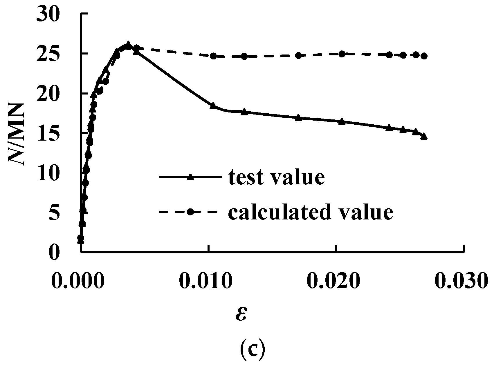
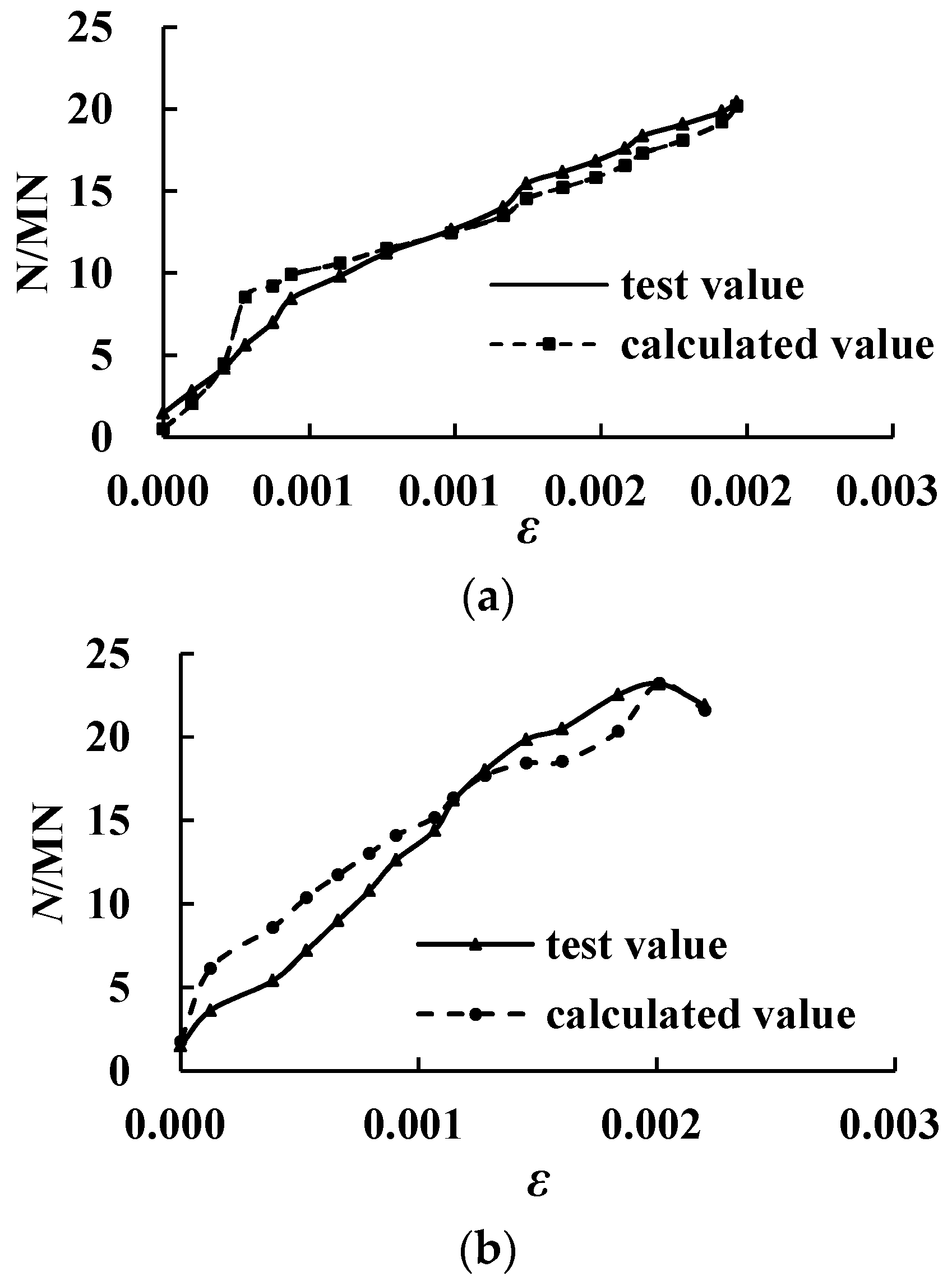
4.3. Numerical Calculation

The ideal elastic-plastic model was considered in the constitutive relation of steel materials [10], including the steel plate and steel bar. The constitutive relations of core concrete were analyzed in Section 4.2, in which Equations (22)–(24) and Equations (42)–(44) were adopted for specimen HGW-1 and HGW-2, and Equations (22)–(25) and Equations (35)–(40) were adopted for specimen HGW-3. Figure 14 shows the constitutive models of steel materials and core concrete. According to the constitutive model of steel materials and core concrete, the stresses of a concrete wall, concrete concealed column, steel plate, and steel bar were calculated utilizing the corresponding strain values, under different loading stages of experiments. Therefore, the shared axial force of each part was obtained, and the sum values of all of the parts were applied in the whole process curve of axial force-strain, the strains of which were derived from displacement values in the experiments. Moreover, the balance and deformation compatibility between the internal and external force were considered in the whole calculation.
Figure 15 shows the calculation and test curves for each specimen, which are basically coincident before the ultimate load, especially when focusing on the ultimate value. So, the constitutive relation of concrete proposed in Section 4.2 can reflect the axial compressive performance of confined concrete. For specimen HGW-3, the calculated value is slightly higher than the experimental value after the ultimate load, which could be explained by the assumption that the axial compressive strain of the concrete coincides with that of the steel plate. However, the strain caused by the axial compressive load, and the strain caused by radical force, which form the axial compressive strain of the specimen, mutually accumulate in the same direction for the steel plate, but cancel each other out in the opposite direction when looking at the concrete. So, the compressive strain of the concrete was smaller than that of the steel plate, and the test value became smaller after the ultimate load.

4.4. Load Bearing Capacity of Composite Wall

For the composite shear wall with the steel plate and concrete, based on the above discussion, the buckling effect of the steel plate, and increasing strength of the confined concrete, should be considered in the calculation of the axial compressive bearing capacity. Taking into account that the mid-high section of the composite wall is the weakest section of the force, the equation of the axial compressive bearing capacity was given as follows:
N = η f y 1 A y 1 + f c c A c + f y 2 A y 2
where fy1 is the yield strength of the steel plate, fy2 is the yield strength of the vertical reinforced bar (for composite wall with built-in steel plate) or internal vertical separator (for composite wall with two skins of steel plate), Ay1 is the cross-sectional area of the steel plate, Ay2 is the cross-sectional area of the vertical reinforced bar or internal vertical separator, fcc is the axial compressive strength of the confined concrete with the method of Section 4.2.1 and Section 4.2.2, an d Ac is the cross-sectional area of the concrete. η is the influence coefficient of the buckling steel plate, where η = 1 for the composite wall with the built-in steel plate. The η value can be obtained using Equation (17) for the composite wall with two skins of steel plate.
Table 4 presents the axial forces of the different parts at the ultimate load, using Equation (45), in which Np is the axial force of the steel plate, Nc is the axial force of the concrete, Ns is the axial force of the vertical reinforced bar or internal vertical separator, Ncal is the sum of axial forces of the different parts, and Ntest is the test axial compressive bearing capacity. In Table 4, the measured strength values are considered in the calculation of the axial force, including Np, Nc, and Ns. For specimen HGW-2, the axial force of the steel plate included the stiffening ribs. For specimen HGW-3, the buckling effect of the steel plate on the axial compression was considered along the long sides, but not the short sides. The calculated values Ncal using Equation (45) are in good agreement with the test values Ntest, with errors no higher than 5%.

5. Conclusions

(1)
The different layout forms of steel plate have a great influence on its buckling, which can affect the bearing capacity of the plate. Under the condition of similar steel ratio, the built-in steel plate buckles later than the yield of the steel plate, and the steel plate is in a state of full-section compression. However, the buckling of the external steel plate occurs earlier than the yield of the steel plate, and the steel plate only yields in the range of effective width at both ends, and demonstrates post-buckling strength.
(2)
The different position of the steel plate forms a different concrete inhibition effect, and the constitutive relation of the concrete is presented by various methods, with key elements of parameter r and the axial compressive strength of the confined concrete fcc. The axial load-strain curves, calculated by a numerical method, are in good agreement with the experimental curves.
(3)
According to the buckling effect of the steel plate, the axial compressive strength increases with confined concrete. The calculated equation for the axial compressive bearing capacity of the composite shear wall, is established, and the calculated results are in good agreement with the experimental results.
(4)
Compared to the composite wall with the unstiffened built-in steel plate, the axial compressive bearing capacity of the composite wall with the external steel plate improved by 28.2%, the elastic plastic deformation capacity increased by 7.1 times, and the steel plate and concrete demonstrated a good cooperative performance.

Acknowledgments

The research was supported by the National Science Foundation of China (Grant No. 51478020). The authors thank Xiaoxu Luo for the assistance in the preparation of the specimens.

Author Contributions

Tingyue Hao conducted the experiments, collected the data, performed the theory analysis, deduced the equations, and wrote the paper. Wanlin Cao contributed to the design of the experiment and the discussion of the results. Qiyun Qiao proposed some good advice in the design of experiment. Yan Liu participated in the process of experiments. Wenbin Zheng participated in writing paper.

Conflicts of Interest

The authors declare no conflict of interest.

References

  1. Wright, H. The Axial Load Behaviour of Composite Walling. J. Constr. Steel Res. 1998, 45, 353–375. [Google Scholar] [CrossRef]
  2. Wright, H.D. Local stability of filled and encased steel sections. J. Struct. Eng. 1995, 121, 1382–1388. [Google Scholar] [CrossRef]
  3. Mydin, M.A.; Wang, Y.C. Structural performance of lightweight steel-foamed concrete-steel composited walling system under compression. Thin-Walled Struct. 2011, 49, 66–76. [Google Scholar] [CrossRef]
  4. Uy, B.; Bradford, M.A. Elastic local buckling of steel plates in composite steel-concrete members. Eng. Struct. 1996, 18, 193–200. [Google Scholar] [CrossRef]
  5. Liang, Q.Q.; Uy, B. Theoretical study on the post-local buckling of steel plates in concrete-filled box columns. Comput. Struct. 2000, 75, 479–490. [Google Scholar] [CrossRef] [Green Version]
  6. Huang, Z.; Liew, J.R. Compressive resistance of steel-concrete-steel sandwich composite walls with J-hook connectors. J. Constr. Steel Res. 2016, 124, 142–162. [Google Scholar] [CrossRef]
  7. Fang, X.; Jiang, B.; Wei, H.; Zhou, Y.; Jiang, Y.; Lai, H. Axial compressive test and study on steel tube confined high strength concrete shear wall. J. Build. Struct. 2013, 34, 100–109. [Google Scholar]
  8. Zhang, Y.; Li, X.; He, Q. Experimental study on local stability of composite walls with steel plates and filled concrete under concentric loads. China Civ. Eng. J. 2016, 49, 62–68. [Google Scholar]
  9. Liu, H. Study on Seismic Behavior of Composite Shear Wall with Double Steel Plates and Infill Concrete with Binding Bars. Ph.D. Thesis, South China University of Technology, Guangzhou, China, May 2013. [Google Scholar]
  10. Guo, Z.; Shi, X. Reinforced Concrete Theory and Analyse; Tsinghua University Press: Beijing, China, 2004. [Google Scholar]
  11. Chen, J. Steel Structure Stability Theory and Design, 6th ed.; Science Press: Beijing, China, 2014. [Google Scholar]
  12. Chen, S. Guide for Stability Design of Steel Structures, 3rd ed.; China Building Industry Press: Beijing, China, 2013. [Google Scholar]
  13. Nie, J.G.; Huang, Y.; Fan, J. Vertical buckling-resistant design of steel plate shear wall structure. Build. Struct. 2010, 4, 002. [Google Scholar]
  14. Mander, J.B.; Priestley, M.J.; Park, R. Theoretical stress-strain model for confined concrete. J. Struct. Eng. 1998, 114, 1804–1826. [Google Scholar] [CrossRef]
  15. Zuo, Z.L.; Cai, J.; Yang, C.; Chen, Q.J.; Sun, G. Axial load behavior of L-shaped CFT stub columns with binding bars. Eng. Struct. 2012, 37, 88–98. [Google Scholar] [CrossRef]
Figure 1. Geometric dimensions. (a) HGW-1; (b) HGW-2; (c) HGW-3.
Applsci 07 00162 g001aApplsci 07 00162 g001b
Figure 2. Stress-strain material curves. (a) steel plate with 16 mm thickness; (b) steel plate with 8 mm thickness; (c) steel plate with 6 mm thickness; (d) steel bar with 14 mm diameter; (e) steel bar with 6 mm diameter; (f) lead wire with 4 mm diameter; (g) stud with 5 mm diameter; (h) concrete.
Applsci 07 00162 g002
Figure 3. Test loading device. (a) Frontal; (b) Lateral; (c) Loading site.
Applsci 07 00162 g003
Figure 4. Strain gauge arrangement. (a) HGW-1 and HGW-2; (b) HGW-3.
Applsci 07 00162 g004
Figure 5. Failure modes. (a) HGW-1; (b) HGW-2; (c) HGW-3.
Applsci 07 00162 g005
Figure 6. Load-displacementcurves. (a) HGW-1 and HGW-2; (b) HGW-3.
Applsci 07 00162 g006
Figure 7. Rigidity degradation curves. (a) HGW-1 and HGW-2; (b) HGW-3.
Applsci 07 00162 g007
Figure 8. Load-strain of steel plate curves.
Applsci 07 00162 g008
Figure 9. Steel strain of HGW-3.
Applsci 07 00162 g009
Figure 10. Schematic diagram of steel plate stress.
Applsci 07 00162 g010
Figure 11. Effective section of plate.
Applsci 07 00162 g011
Figure 12. Force diagrams of steel plate. (a) short side; (b) long side.
Applsci 07 00162 g012
Figure 13. Area of confined concrete district.
Applsci 07 00162 g013
Figure 14. Constitutive model. (a) Steel material (b) Core concrete.
Applsci 07 00162 g014
Figure 15. Comparison between the numerical results and experimental results. (a) HGW-1; (b) HGW-2; (c) HGW-3.
Applsci 07 00162 g015aApplsci 07 00162 g015b
Table 1. Mechanical properties of the steel materials.
TypeDimensions/mmfy/MPafu/MPaδ/%Es/MPa
Steel plate16 (thickness)33353217.382.06 × 105
Steel plate8 (thickness)37649824.302.09 × 105
Steel plate6 (thickness)37452026.512.02 × 105
Steel bar14 (diameter)45345830.602.02 × 105
Steel bar6 (diameter)38538632.202.02 × 105
Lead wire4 (diameter)35946834.102.04 × 105
stud5 (diameter)636---
Table 2. Characteristic values.
Specimen No.Crack LoadYield LoadUltimate LoadFailure Load
N/MNΔcr/mmN/MNΔy/mmN/MNΔp/mmN/MNΔu/mm
HGW-13.60.46320.463.53520.463.535
HGW-25.40.69723.203.61721.913.960
HGW-321.632.92726.147.50319.4220.743
Table 3. Buckling stress of specimens.
Specimen No.Calculated Buckling Stress (N/mm2)Test Buckling Stress (N/mm2)Yield Stress (N/mm2)η
HGW-1133333333-
HGW-2689-333-
HGW-33023113760.719
Table 4. Axial forces of different parts at ultimate load.
Specimen No.Np/kNNc/kNNs/kNNcal/kNNtest/kNNcal/Ntest
HGW-1639412,349139420,09220,4270.984
HGW-2729615,037139423,72723,2031.023
HGW-3689917,340127525,51426,1390.976

