Time Series Prediction Based on Adaptive Weight Online Sequential Extreme Learning Machine

Abstract

A novel adaptive weight online sequential extreme learning machine (AWOS-ELM) is proposed for predicting time series problems based on an online sequential extreme learning machine (OS-ELM) in this paper. In real-world online applications, the sequentially coming data chunk usually possesses varying confidence coefficients, and the data chunk with a low confidence coefficient tends to mislead the subsequent training process. The proposed AWOS-ELM can improve the training process by accessing the confidence coefficient adaptively and determining the training weight accordingly. Experiments on six time series prediction data sets have verified that the AWOS-ELM algorithm performs better in generalization performance, stability, and prediction ability than the OS-ELM algorithm. In addition, a real-world mechanical system identification problem is considered to test the feasibility and efficacy of the AWOS-ELM algorithm.

1. Introduction

Time series prediction technology has already been studied over the past few decades, and a large amount of applications have been reported in a wide range of fields, such as weather forecasting [1], stock market prediction [2], communication signal processing [3], sales forecasting [4], and so on. On account of the frequent applications of time series predictions, plenty of predicting methods have been developed. Gooijer and Hyndman gave an overview of various predicting methods and indicated the future directions for time series prediction problems [5]. In particular, the classical statistical linear method, an autoregressive integrated moving average model (ARIMA) based modeling method, is still widely adopted and the complete methodology is able to be found in Box’s and Jenkins’s remarkable contribution [6]. However, the predicting accuracy of classical statistical methods suffer from the nonlinearity and complexity of many real time series. For this reason, some computational intelligence methods which may outperform classical statistical methods in many complex nonlinear problems have emerged [7,8].

Artificial neural network (ANN) methods have attracted extensive attention in the time series prediction field [9]. ANNs are universal nonlinear regression techniques, and are able to be applied into time series prediction conveniently [10]. Furthermore, compared with classical methods, the assumptions for prediction can be relaxed by ANNs, such as Gaussian distribution of noise and the linearity of the model. In contrast to the fact that the model hyperparameters of the ARIMA model is required to be fine-tuned for good prediction, this complication is able to be avoided by ANNs [11]. The hyperparameters of the ARIMA model are quite often adjusted according to domain knowledge, while the ANNs model usually can obtain competitive results without any domain knowledge [12].

For some situations where intensive human adjustment is not affordable, ANNs and other computational intelligence methods are usually better than classical statistical methods. Kumar investigated neural network models for forecasting the Indian stock market index [13]. Yoon discussed integrating ANN and support vector machine (SVM) methods for long-term prediction, and the stability and accuracy are improved [14]. Nevertheless, since the neural networks used by Kumar and Yoon are obtained in an iterative way by means of gradient-based algorithms, the diagnosis systems suffer from time-consuming problems.

Extreme learning machine (ELM) is a high-efficiency learning algorithm for single-hidden layer feedforward neural network (SLFN), and it has been proven to have classification capacity and universal approximation capacity [15]. In addition, Huang has shown that the hidden-layer parameters can be randomly assigned, and then the output weight is able to be computed analytically [16]. It has been verified that ELM costs much less training time and has better or similar generalization performance than SVM and traditional neural networks [17]. Hosseinioun presented the use of wavelet transform and adaptive ELM to forecast outlier occurrence in stock market time series [18]. Dash presented an optimized ELM for predicting financial time series [19]. The ELM based prediction methods have high accuracy and fast learning speed in off-line cases, but they are not suitable for online applications. Liang et al. proposed OS-ELM by incorporating a sequential learning algorithm with ELM [20]. Compared with conventional online training methods, OS-ELM tends to have a faster training speed and better generalization performance. However, in lots of real-world online applications, the confidence coefficient of a sequential data chunk may be disturbed by measurement noise and external disturbance. If the data chunk with low confidence coefficient is employed in the learning process in a normal way, the accuracy of the trained network is likely to be reduced. In this paper, the AWOS-ELM algorithm is proposed to reduce the negative influence of data chunks with low confidence coefficients, where the confidence coefficient of each data chunk is assessed before being used to train the network, and the weight of each data chunk is obtained according to the assessed confidence coefficient. Experiments on six time series prediction problems and a mechanical system identification problem have verified that the AWOS-ELM algorithm performs better in generalization performance, stability, and predictability than the OS-ELM algorithm.

This manuscript is organized as follows. In Section 2, the basic concepts and related works of optimization ELM and OS-ELM algorithms are reviewed briefly. The integrated structure of the proposed algorithm and the formula derivation is given in Section 3. In Section 4, the performance evaluation of the AWOS-ELM is carried out on six time series prediction problems and a mechanical system identification problem. The conclusion is drawn in Section 5.

2. Preliminaries

In this section, with the purpose of offering preliminaries pertinent to the proposed AWOS-ELM algorithm, the optimization of ELM and OS-ELM is reviewed briefly. OS-ELM, an online learning algorithm on the basis of classical ELM, was proposed by Liang in 2006 for training sequential data. Huang further developed the classical ELM into the optimization ELM according to the Karush-Kuhn-Tucker (KKT) theory and optimization theory in 2012 [21]. Compared to the classical ELM, the regularization parameters are used in the optimization ELM to increase the accuracy and generation performance. The OS-ELM in this paper also employs the regularization parameters according to Huang’s theory.

2.1. Optimization Extreme Learning Machine

ELM is a high-efficiency SLFN learning algorithm, where the hidden node parameters can be assigned randomly. Assume that there are N different training data ${\left\{\left(x_i,t_i\right)\right\}}_{i=1}^N\subset {\Re }^n\times {\Re }^m$ for the supervised learning process, where $x_i={\left[x_{i1},x_{i2},\dots ,x_{in}\right]}^T\in {\Re }^n$ and $t_i={\left[t_{i1},t_{i2},\dots ,t_{im}\right]}^T\in {\Re }^m$ are the input vector and output vector, respectively, and the mathematical model of SLFNs is described as:

$$f_L\left(x\right)={\displaystyle \sum _{i=1}^L{\mathsf{\beta }}_{i}g\left({\mathsf{\omega }}_i,b_i,x\right)},x\in {\Re }^n$$

(1)

where ${\mathsf{\omega }}_i\in {\Re }^n$, $b_i\in \Re$ and ${\mathsf{\beta }}_i={\left[{\beta }_{i1},{\beta }_{i2},\dots ,{\beta }_{im}\right]}^T\in {\Re }^m$ denote the ith hidden node parameters, $L$ is the hidden nodes number, and $g\left({\mathsf{\omega }}_i,b_i,x\right)$ represents the hidden-layer output in accordance with the input $x$. If the $N$ training samples are absolutely approximated by the SLFNs with $L$ hidden nodes, it indicates the following equation:

$${\displaystyle \sum _{i=1}^L{\mathsf{\beta }}_{i}g\left({\mathsf{\omega }}_i,b_i,x\right)}=t_j,j=1,2,\dots ,N$$

(2)

Equation (2) is able to be described compactly as the following equation:

$$H\mathsf{\beta }=T$$

(3)

where

$$H\left({\mathsf{\omega }}_1,\dots ,{\mathsf{\omega }}_L,b_1,\dots ,b_L,x_1,\dots ,x_N\right)={\left[\begin{array}{ccc}g\left({\mathsf{\omega }}_1,b_1,x_1\right)& \cdots & g\left({\mathsf{\omega }}_L,b_L,x_1\right)\\ ⋮& \ddots & ⋮\\ g\left({\mathsf{\omega }}_1,b_1,x_N\right)& \cdots & g\left({\mathsf{\omega }}_L,b_L,x_N\right)\end{array}\right]}_{N\times L}$$

(4)

$$\mathsf{\beta }={\left[\begin{array}{c}{\mathsf{\beta }}_1^T\\ ⋮\\ {\mathsf{\beta }}_L^T\end{array}\right]}_{L\times m}\mathrm{and}T={\left[\begin{array}{c}{t}_1^T\\ ⋮\\ t_N^T\end{array}\right]}_{N\times m}$$

(5)

Traditionally, for the purpose of training an SLFN, one needs to find specific ${\mathsf{\omega }}_i,b_i,{\mathsf{\beta }}_i,i=1,\dots ,L$, such that $\Vert H\mathsf{\beta }-T\Vert$ takes a minimum value. If $H$ is unknown, the gradient-based approaches are usually employed to iteratively adjust ${\mathsf{\omega }}_i,b_i,{\mathsf{\beta }}_i$. However, for most applications, the gradient-based method is extremely time-consuming and often stop at the local minimum. According to the theory of Huang, the hidden-layer learning parameters ${\mathsf{\omega }}_i$ and $b_i$ can be assigned randomly, and as such the SLFN is able to approximate any target function universally as soon as the activation function is nonzero, the target function is continuous and the input sets are compact [17]. If $L\le N$, the column rank of $H$ is full with probability one, and in real-world applications, the condition $L\le N$ can be easily satisfied. Considering the norm of the output weight $\mathsf{\beta }$ to be part of the cost function [22], the optimization ELM model can be represented as:

$$\begin{array}{l}\min :L_{elm}=\frac{1}{2}{\Vert \mathsf{\beta }\Vert }^2+\frac{C}{2}{\displaystyle \sum _{i=1}^N{\Vert {\mathsf{\epsilon }}_i\Vert }^2}\\ st:h\left(x_i\right)\mathsf{\beta }=t_i-{\mathsf{\epsilon }}_i,i=1,2,\dots ,N\end{array}$$

(6)

where ${\mathsf{\epsilon }}_i$ is the prediction error of the ith training sample. Because the convex optimization problem does not have an inequality constraint, the Slater’s condition is satisfied and the strong duality holds. Consequently, on the basis of the KKT theorem, Equation (6) can be represented as follows:

$$\min :L_{elm}=\frac{1}{2}{\Vert \mathsf{\beta }\Vert }^2+\frac{C}{2}{\displaystyle \sum _{i=1}^N{\mathsf{\epsilon }}_i^2}-{\displaystyle \sum _{i=1}^N{\mathsf{\alpha }}_i\left(h\left(x_i\right)\mathsf{\beta }-t_i+{\mathsf{\epsilon }}_i\right)}$$

(7)

where ${\mathsf{\alpha }}_i$ is the Lagrange multiplier. By optimizing Equation (7), the output weight can be obtained as follows:

$$\mathsf{\beta }={\left(\frac{I}{C}+H^{T}H\right)}^{-1}{H}^{T}T$$

(8)

Since the output weights $\mathsf{\beta }$ is computed analytically, compared with traditional iterative implementations of SLFNs, the optimization ELM has similar generalization performance and dramatically increased running speed.

2.2. Online Sequential Extreme Learning Machine

In many practical instances, the sequential training samples $\aleph =\left\{\left(x_i,t_i\right)|x_i\in {\Re }^n,t_i\in {\Re }^m,i=1,2,\dots \right\}$ are produced chunk by chunk, and the chunk size may be fixed or various. Assume that the jth data chunk has $N_j$ samples, then the chunk at time k is able to be represented as ${\aleph }_k={\left\{\left(x_i,t_i\right)\right\}}_{i=\left({\displaystyle \sum _{j=0}^{k-1}{N}_j}\right)+1}^{{\displaystyle \sum _{j=0}^k{N}_j}}$. The initialization of the learning process is carried out according to a small data chunk ${\aleph }_0={\left\{\left(x_i,t_i\right)\right\}}_{i=1}^{N_0}$, where $N_0$ is the samples number of data chunk ${\aleph }_0$, and $N_0$ ought to be equal to or greater than $L$. With The hidden-layer parameters $\left({\mathsf{\omega }}_i,b_i\right),i=1,2,\dots ,L$ assigned into random values, the initial $H_0$ can be computed as the following equation:

$$H_0:=H\left({\mathsf{\omega }}_1,\dots ,{\mathsf{\omega }}_L,b_1,\dots ,b_L,x_1,\dots ,x_{N_0}\right)$$

(9)

and then the initial ${\mathsf{\beta }}_0$ is able to be obtained according to ELM as follows:

$${\mathsf{\beta }}_0=P_0{H}_0^T{T}_0$$

(10)

where $P_0={\left(\frac{I}{C}+H_0^T{H}_0\right)}^{-1}$ and $T_0={\left[t_1,\dots ,t_{N_0}\right]}^T$.

The partial hidden-layer output matrixes $h_{k+1}$ and the partial output-layer matrixes $t_{k+1}$ corresponding to data chunk at time k + 1 are respectively defined as:

$$h_{k+1}:=H\left({\mathsf{\omega }}_1,\dots ,{\mathsf{\omega }}_L,b_1,\dots ,b_L,x_{\left({\displaystyle {\sum }_{j=0}^k{N}_j}\right)+1},\dots ,x_{{\displaystyle {\sum }_{j=0}^{k+1}{N}_j}}\right)$$

(11)

$$t_{k+1}:={\left[t_{\left({\displaystyle {\sum }_{j=0}^k{N}_j}\right)+1},\dots ,t_{{\displaystyle {\sum }_{j=0}^{k+1}{N}_j}}\right]}^T$$

(12)

Then $H_k$ and $T_k$ can be respectively expressed as:

$$H_k=H\left({\mathsf{\omega }}_1,\dots ,{\mathsf{\omega }}_L,b_1,\dots ,b_L,x_1,\dots ,x_{{\displaystyle {\sum }_{j=0}^k{N}_j}}\right),T_k=\left[\begin{array}{c}{t}_1^T\\ ⋮\\ t_{{\displaystyle {\sum }_{j=0}^k{N}_j}}^T\end{array}\right]$$

(13)

and we have

$$H_{k+1}=\left[\begin{array}{c}{H}_k\\ h_{k+1}\end{array}\right],T_{k+1}=\left[\begin{array}{c}{T}_k\\ t_{k+1}^T\end{array}\right]$$

(14)

The least squares solution of $H_{k+1}\mathsf{\beta }=T_{k+1}$ should be the output weight at time k + 1, ${\mathsf{\beta }}_{k+1}$ and it is able to be computed in an iterative way as follows:

$${\mathsf{\beta }}_{k+1}={\mathsf{\beta }}_k+P_{k+1}{h}_{k+1}^T\left(t_{k+1}^T-h_{k+1}{\mathsf{\beta }}_k\right)$$

(15)

$$P_{k+1}=P_k-P_k{h}_{k+1}^T{\left(I+h_{k+1}{P}_k{h}_{k+1}^T\right)}^{-1}{h}_{k+1}{P}_k$$

(16)

OS-ELM is composed of an initialization phase and sequential learning phase and need not retain all the historic data. In the initialization phase, $H_0$, ${\mathsf{\beta }}_0$, $P_0$, and $T_0$ are initialized for the use in the sequential learning phase. The samples number of the initialization chunk should be equal to or greater than the hidden nodes number. In the sequential learning phase, the sequential date chunk is commenced on iteratively. Once the training process on the latest coming data chunk is completed, the historic data can be discarded and not used any more. From the derivation of OS-ELM, it is easy to find that OS-ELM and ELM have similar generalization performances. In fact, the ELM algorithm is a specific example of the OS-ELM algorithm if all of the training samples are processed in the initialization of the learning process.

3. The Proposed Adaptive Weight Online Sequential Extreme Learning Machine

In lots of real online applications, with measurement noise and unexpected external disturbance, the sequential data chunks often have varying confidence coefficients. It can be easily found that OS-ELM cannot deal with the varying confidence coefficients very well. If a data chunk with a low confidence coefficient is employed to train the network in the normal way, the accuracy of the trained network is likely to be reduced. In this section, we propose the novel AWOS-ELM, where the confidence coefficient of each data chunk is assessed before being used to train the network, and the weight of each data chunk is obtained accordingly.

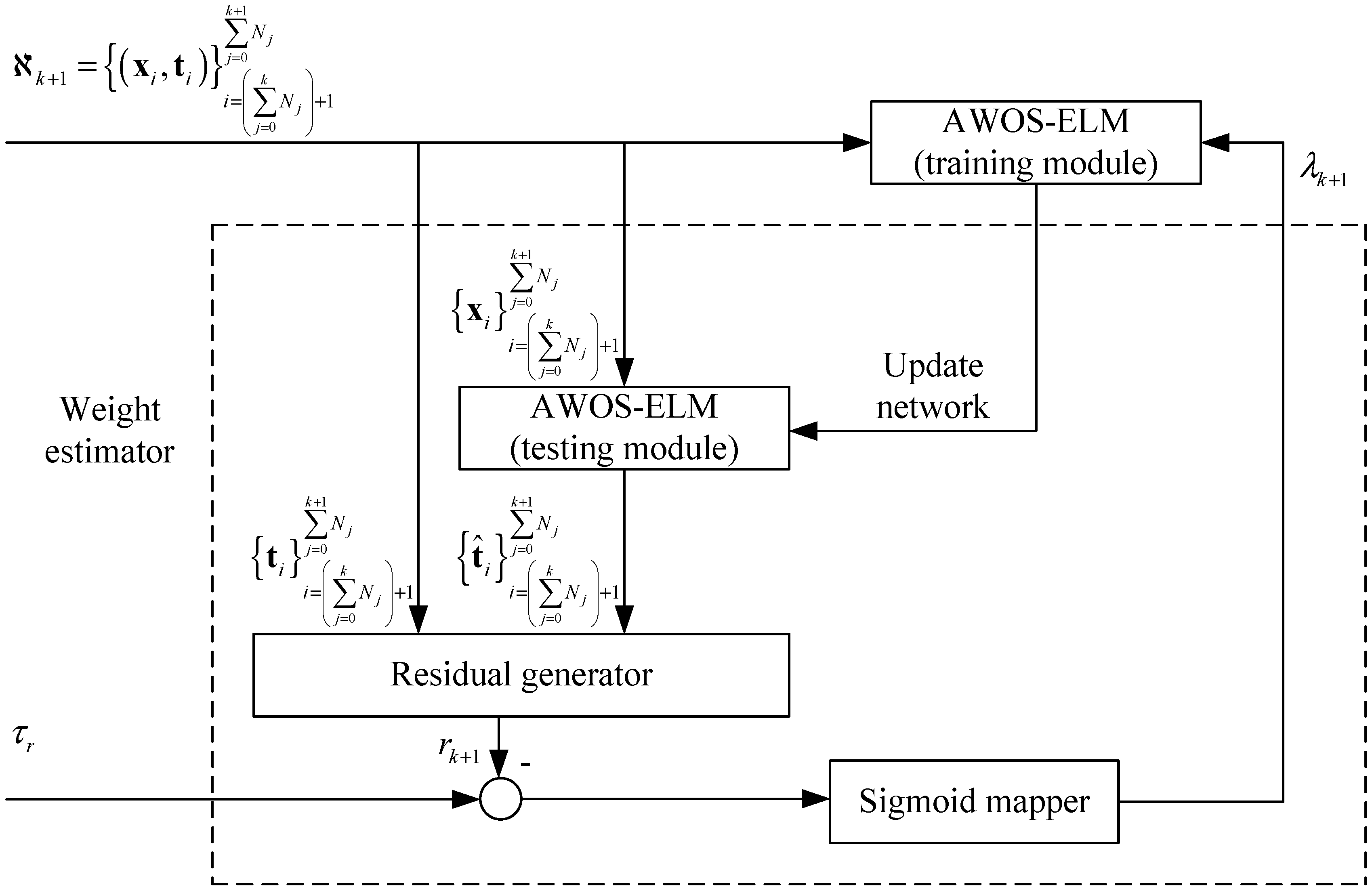
3.1. Integrated Structure

The block diagram of AWOS-ELM algorithm is given in Figure 1. When the new sequential sample ${\aleph }_{k+1}={\left\{\left(x_i,t_i\right)\right\}}_{i=\left({\displaystyle \sum _{j=0}^k{N}_j}\right)+1}^{{\displaystyle \sum _{j=0}^{k+1}{N}_j}}$ arrives, the weight estimator accesses the confidence coefficient of ${\aleph }_{k+1}$ and determines the corresponding weight ${\lambda }_{k+1}$. Then the training module of AWOS-ELM algorithm utilizes ${\lambda }_{k+1}$ and ${\aleph }_{k+1}$ to train the network. The weight estimator includes an AWOS-ELM testing module, residual generator and sigmoid function. The testing module produces the prediction value ${\left\{{\widehat{t}}_i\right\}}_{i=\left({\displaystyle \sum _{j=0}^k{N}_j}\right)+1}^{{\displaystyle \sum _{j=0}^{k+1}{N}_j}}$ according to the input vector ${\left\{x_i\right\}}_{i=\left({\displaystyle \sum _{j=0}^k{N}_j}\right)+1}^{{\displaystyle \sum _{j=0}^{k+1}{N}_j}}$. The residual $r_{k+1}$ is produced by the residual generator according to the comparison between the prediction value ${\left\{{\widehat{t}}_i\right\}}_{i=\left({\displaystyle \sum _{j=0}^k{N}_j}\right)+1}^{{\displaystyle \sum _{j=0}^{k+1}{N}_j}}$ and the target value ${\left\{t_i\right\}}_{i=\left({\displaystyle \sum _{j=0}^k{N}_j}\right)+1}^{{\displaystyle \sum _{j=0}^{k+1}{N}_j}}$, where the residual $r_{k+1}$ is defined as the following:

$$r_{k+1}=\sqrt{\frac{{\displaystyle \sum _{i=1}^{N_{k+1}}{\Vert {\widehat{t}}_{i+{\displaystyle \sum _{j=0}^k{N}_j}}-t_{i+{\displaystyle \sum _{j=0}^k{N}_j}}\Vert }_F^2}}{N_{k+1}\times m}}$$

(17)

where $m$ is the dimension of the output vector $t_i$. Then the sigmoid mapper produce the accessed weight ${\lambda }_{k+1}$ according to the difference between ${\tau }_r$ and $r_{k+1}$ as the following:

$${\lambda }_{k+1}=\frac{1}{1+e^{-\phi ({\tau }_r-r_{k+1})}}$$

(18)

where ${\tau }_r$ is the threshold value and $\phi$ is a scaling factor which can represent the gradient of the sigmoid function at the threshold point. For the samples with the residuals closer to the threshold ${\tau }_r$, the greater the $\phi$ is, the greater the difference between calculated weights will be. Moreover, $\phi$ is manually selected to be 500 according to the performance in this paper. As observed from Equation (18), the greater the residual $r_{k+1}$ is, the less the accessed weight ${\lambda }_{k+1}$ is, and $0<{\lambda }_k<1$. The network of the testing module should be updated according to the training module before next sequential data chunk is incoming. The abnormal samples which cannot match the normal model well will have low accessed weight, and their negative impact to the subsequent learning process will be reduced. Thus, the AWOS-ELM algorithm is able to properly handle the varying confidence coefficients of each data chunk.

3.2. Formula Derivation

The assessed weight of the data chunk at time k is ${\lambda }_k$, then ${\mathsf{\beta }}_{k+1}^{\prime }$ is the least squares solution of the following equation:

$$\left[\begin{array}{c}{\lambda }_0{H}_0\\ {\lambda }_1{h}_1\\ ⋮\\ {\lambda }_{\mathrm{k}+1}{h}_{k+1}\end{array}\right]{\mathsf{\beta }}^{\prime }=\left[\begin{array}{c}{\lambda }_0{T}_0\\ {\lambda }_1{t}_1^T\\ ⋮\\ {\lambda }_{\mathrm{k}+1}{t}_{k+1}^T\end{array}\right]$$

(19)

Let $H_{k+1}^{\prime }:=\left[\begin{array}{c}{H}_k^{\prime }\\ {\lambda }_{k+1}{h}_{k+1}\end{array}\right]$, $H_0^{\prime }:={\lambda }_0{H}_0$, $T_{k+1}^{\prime }:=\left[\begin{array}{c}{T}_k^{\prime }\\ {\lambda }_{k+1}{t}_{k+1}^T\end{array}\right]$, $T_0^{\prime }:={\lambda }_0{T}_0$, then Equation (19) can be described in a compact way as:

$$H_{k+1}^{\prime }{\mathsf{\beta }}^{\prime }=T_{k+1}^{\prime }$$

(20)

Theorem 1.

The solution of Equation (20) in the sense of least squares is able to be obtained in an iterative way as follows:

$${\mathsf{\beta }}_{k+1}^{\prime }={\mathsf{\beta }}_k^{\prime }+K_{k+1}\left(t_{k+1}-h_{k+1}{\mathsf{\beta }}_k^{\prime }\right)$$

(21)

$$P_{k+1}^{\prime }=\left(I-K_{k+1}{h}_{k+1}\right)P_k^{\prime }$$

(22)

$$K_{k+1}=P_k^{\prime }{h}_{k+1}{\left(\frac{I}{{\lambda }_{k+1}^2}+h_{k+1}{P}_k^{\prime }{h}_{k+1}^T\right)}^{-1}$$

(23)

where $P_k^{\prime }:={\left({H^{\prime }}_k^T{H}_k^{\prime }\right)}^{-1}$, ${\mathsf{\beta }}_k^{\prime }=P_k^{\prime }{H^{\prime }}_k^T{T}_k^{\prime }$.

Proof. 

According to the definition of $P_k^{\prime }$, $P_{k+1}^{\prime }$ can be found as follows:

$$P_{k+1}^{\prime }={\left({\left[\begin{array}{c}{H}_k^{\prime }\\ {\lambda }_{k+1}{h}_{k+1}\end{array}\right]}^T\left[\begin{array}{c}{H}_k^{\prime }\\ {\lambda }_{k+1}{h}_{k+1}\end{array}\right]\right)}^{-1}={\left({H^{\prime }}_k^T{H}_k^{\prime }+{\lambda }_{k+1}^2{h}_{k+1}^T{h}_{k+1}\right)}^{-1}$$

(24)

Apply the Sherman-Morrison-Woodbury formula [23] into Equation (24), and then $P_{k+1}^{\prime }$ can be determined iteratively as follows:

$$\begin{array}{lll}{P}_{k+1}^{\prime }& =& P_k^{\prime }-P_k^{\prime }{h}_{k+1}^T{\left(\frac{I}{{\lambda }_{k+1}^2}+h_{k+1}{P}_k^{\prime }{h}_{k+1}^T\right)}^{-1}{h}_{k+1}{P}_k^{\prime }\\ & =& P_k^{\prime }-K_{k+1}{h}_{k+1}{P}_k^{\prime }\end{array}$$

(25)

According to Equation (25) and ${\mathsf{\beta }}_{k+1}^{\prime }=P_{k+1}^{\prime }{H^{\prime }}_{k+1}^T{T}_{k+1}^{\prime }$, the output matrix ${\mathsf{\beta }}_{k+1}^{\prime }$ can be obtained from the following equation:

$$\begin{array}{lll}{\mathsf{\beta }}_{k+1}^{\prime }& =& \left(P_k^{\prime }-K_{k+1}{h}_{k+1}{P}_k^{\prime }\right){\left[\begin{array}{c}{H}_k^{\prime }\\ {\lambda }_{k+1}{h}_{k+1}\end{array}\right]}^T\left[\begin{array}{c}{T}_k^{\prime }\\ {\lambda }_{k+1}{t}_{k+1}^T\end{array}\right]\\ & =& \left(P_k^{\prime }-K_{k+1}{h}_{k+1}{P}_k^{\prime }\right)\left({H^{\prime }}_k^T{T}_k^{\prime }+{\lambda }_{k+1}^2{h}_{k+1}^T{t}_{k+1}^T\right)\\ & =& P_k^{\prime }{H^{\prime }}_k^T{T}_k^{\prime }-K_{k+1}{h}_{k+1}{P}_k^{\prime }{H^{\prime }}_k^T{T}^{\prime }\\ & & +{\lambda }_{k+1}^2\left(P_k^{\prime }{h}_{k+1}^T-K_{k+1}{h}_{k+1}{P}_k^{\prime }{h}_{k+1}^T\right)t_{k+1}^T\\ & =& {\mathsf{\beta }}_k^{\prime }-K_{k+1}{h}_{k+1}{\mathsf{\beta }}_k^{\prime }\\ & & +{\lambda }_{k+1}^2\left(P_k^{\prime }{h}_{k+1}^T-K_{k+1}{h}_{k+1}{P}_k^{\prime }{h}_{k+1}^T\right)t_{k+1}^T\end{array}$$

(26)

Then we can simplify the $P_k^{\prime }h{(k+1)}^T-K_{k+1}h(k+1)P_k^{\prime }h{(k+1)}^T$ in Equation (26) as:

$$\begin{array}{l}{P}_k^{\prime }{h}_{k+1}^T-K_{k+1}{h}_{k+1}{P}_k^{\prime }{h}_{k+1}^T\\ =P_k^{\prime }{h}_{k+1}^T-K_{k+1}{h}_{k+1}{P}_k^{\prime }{h}_{k+1}^T-\frac{K_{k+1}}{{\lambda }_{k+1}^2}+\frac{K_{k+1}}{{\lambda }_{k+1}^2}\\ =P_k^{\prime }{h}_{k+1}^T-K_{k+1}\left(\frac{I}{{\lambda }_{k+1}^2}+h_{k+1}{P}_k^{\prime }{h}_{k+1}^T\right)+\frac{K_{k+1}}{{\lambda }_{k+1}^2}\\ =\frac{K_{k+1}}{{\lambda }_{k+1}^2}\end{array}$$

(27)

Substituting Equation (27) into Equation (26), ${\mathsf{\beta }}_{k+1}^{\prime }$ is able to be determined in a compact way as:

$${\mathsf{\beta }}_{k+1}^{\prime }={\mathsf{\beta }}_k^{\prime }+K_{k+1}\left(t_{k+1}^T-h_{k+1}{\mathsf{\beta }}_k^{\prime }\right)$$

(28)

Proposed AWOS-ELM Algorithm: 

If $L$ and $\mathrm{g}:\Re \to \Re$ are given, the AWOS-ELM algorithm is able to be summarized as follows:

Step 1. Initialization phase: choose the initial data chunk ${\aleph }_0={\left\{\left(x_i,t_i\right)\right\}}_{i=1}^{N_0}$, where $N_0\ge L$.

(1)

Configure the learning parameters $\left({\mathsf{\omega }}_i,b_i\right),i=1,2,\dots ,L$ randomly, and set ${\lambda }_0=1$;

(2)

Calculate $H_0$ and ${\mathsf{\beta }}_0$ according to Equations (9) and (10);

(3)

Set $k=0$.

Step 2. Sequential learning phase: iteratively train the network using the data chunk at time k+1 ${\aleph }_{k+1}={\left\{\left(x_i,t_i\right)\right\}}_{i=\left({\displaystyle {\sum }_{j=0}^k{N}_j}\right)+1}^{{\displaystyle {\sum }_{j=0}^{k+1}{N}_j}}$;

(1)

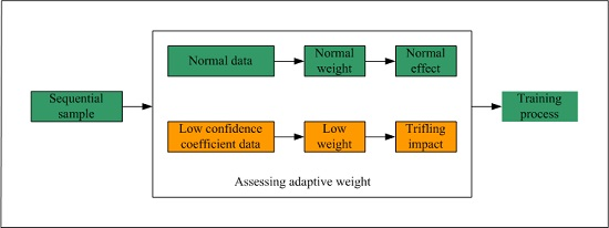
Assess the confidence coefficient of this new data chunk according to the test module in Figure 1, and determine the corresponding weight ${\lambda }_{k+1}$;

(2)

Calculate the partial $h_{k+1}$ and $t_{k+1}$as Equations (11) and (12);

(3)

Compute ${\mathsf{\beta }}_{k+1}^{\prime }$ in an iterative way in accordance with Equations (21)–(23);

(4)

Set $k=k+1$ and go to Step 2 until all the training data chunks are used for the learning process.

Remark 1.

Actually, the AWOS-ELM is the OS-ELM algorithm with adaptive weight. As a new data chunk comes, the proposed algorithm need not repeat the training process of ELM. The AWOS-ELM uses the newly arriving data chunk and the known information which is learned before to conduct the update of the training network, while the ELM applies all data chunks to update the network parameters. Therefore, in the case of sequential predicting problems, the AWOS-ELM algorithm tends to produce a better training process than the ELM algorithm.

Remark 2.

In the learning process by AWOS-ELM, since the confidence coefficient of each data chunk varies with time, the weight of each data chunk is assessed as soon as the new training data arrives at the next unit time and the SLFN will be trained accordingly. Therefore, the learning process can aptly deal with the confidence coefficient of each data chunk.

Remark 3.

If ${\lambda }_0={\lambda }_1=\cdots ={\lambda }_k=\cdots$, that is, each training data chunk has the same assessed weight, then it is obvious that AWOS-ELM is equivalent to OS-ELM, indicating that the OS-ELM is a special case of the AWOS-ELM algorithm.

4. Experiments

For the purpose of verifying the validity of the proposed AWOS-ELM algorithm, six benchmark data sets and an identification problem on the dynamics of a flexible robot arm are considered in this section for the performance comparison between the OS-ELM and AWOS-ELM algorithm. The attributes of each dataset are uniformed into the range [−1,1], and the corresponding outputs are uniformed into [0,1]. The software environment for all experiments is MATLAB 7.11 (MathWorks, Natick, MA, USA) and the hardware environment is an ordinary PC with Intel Core i5-3210M processor. With the purpose of obtaining reliable statistical results, fifty trials are carried out for each case. For the purpose of comparing the performance, the definition of the rooted mean squared errors (RMSE) is given as follows:

$$RMSE=\sqrt{\frac{{\displaystyle \sum _{i=1}^{N_{testing}}{\Vert {\widehat{t}}_i-t_i\Vert }_F^2}}{N_{testing}\times m}}$$

(29)

where ${\widehat{t}}_i$ is the prediction value in regard to the target value $t_i$, $N_{testing}$ denotes the testing samples number. For a learning algorithm, a smaller RMSE often indicates a better generalization performance. In addition, $\sigma$, the standard deviation of RMSEs in 50 trials, can effectively reflect the reliability of the proposed algorithm. Two classical hidden node functions, the radial basis function $h\left(x\right)=e^{-b_i{\Vert x-a_i\Vert }^2}$ and the sigmoid function $h\left(x\right)=\frac{1}{1+e^{-\left(a_i\cdot x+b_i\right)}}$, are chosen for each learning algorithm. If the hidden function is set to be sigmoid, ${\mathsf{\omega }}_i$ and $b_i$ are chosen according to uniform distribution in the closed interval [−1,1], and if the RBF function is selected, ${\mathsf{\omega }}_i$ is also obtained from the uniform distribution in [−1,1], while $b_i$ is determined according to the uniform distribution in the open interval (0,0.5) [15]. For the AWOS-ELM algorithm, we select the threshold ${\tau }_r$ from the domain $\left\{x|x=0.02+0.01k,k=0,1,2,\cdots 18\right\}$, and the best threshold is selected manually according to the prediction performance. In addition, the regulation parameter is set as $C={10}^{-5}$ [24]. In order to verify the prediction performance of AWOS-ELM with the existence of disturbance, Gaussian noise with a standard deviation of 0.0015 is added into the training samples. For the purpose of having a fair comparison, the hidden nodes number of OS-ELM is optimized by the cross validation method, afterwards the optimized hidden nodes number is extended to the AWOS-ELM algorithm.

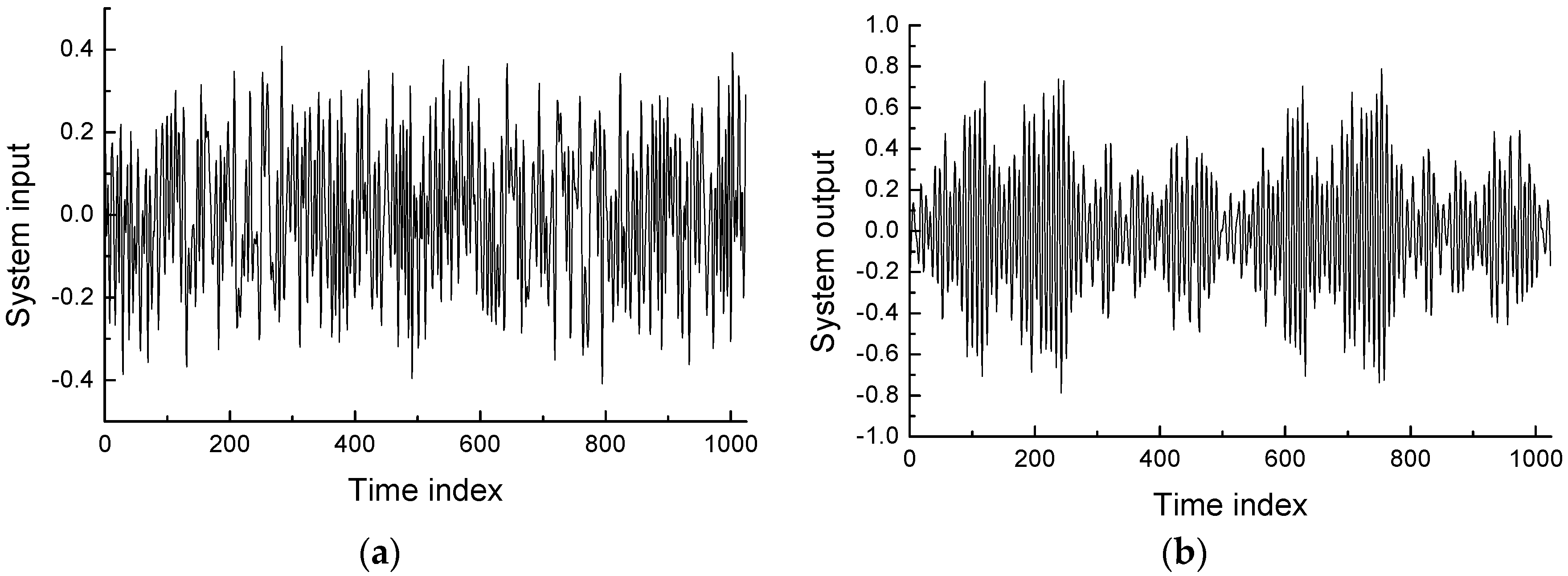
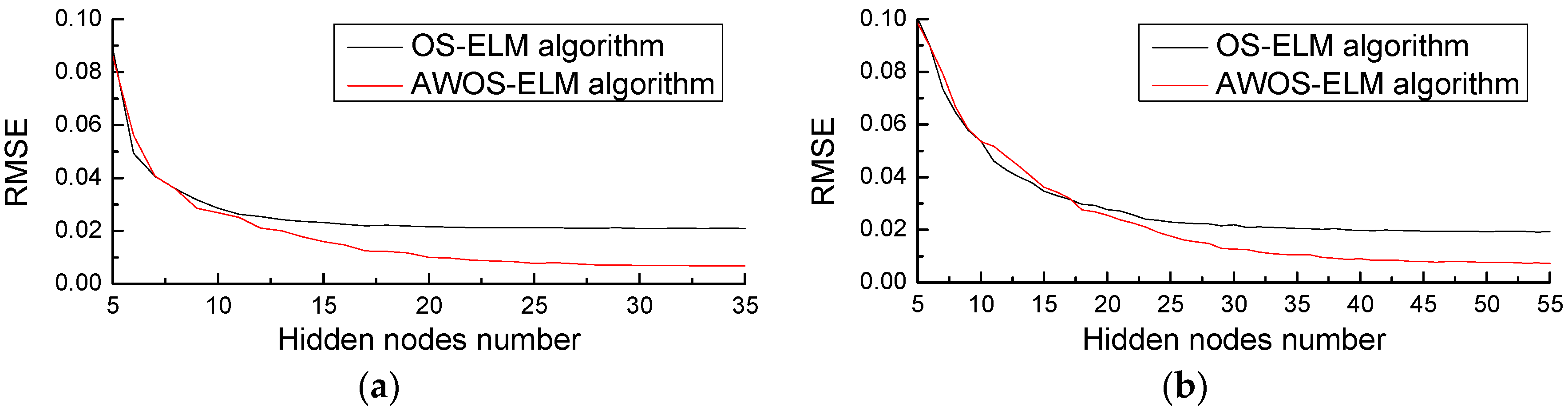
4.1. Benchmark Data Sets

In this subsection, we make a comparison between AWOS-ELM and OS-ELM on six time series prediction problems consisting of three artificial time series and three actual time series. Among them, a monthly milk production dataset, having 100 training and 44 testing data, and an electricity production dataset, having 350 training and 102 testing data, are obtained from the well-known Time Series Data Library. The sunspot time series, having 2500 training and 690 testing data, is the monthly mean total sunspot number from January 1749 to December 2015 and is obtained from Solar Influences Data Analysis Center. Pseudo periodic synthetic time series, having 8000 training and 1801 testing data, is found from the University of California, Irvine (UCI) repository. The other two chaotic series, viz. Mackey-Glass and Logistic time series, are generated according to mathematical equations. The Mackey-Glass series $\left\{x_k^{mg}|k=1,2,3,\dots \right\}$ is generated according to the following differential delay equation [25]

$$\frac{d{x}^{mg}\left(t\right)}{dt}=\frac{a\left(t-\tau \right)}{1+x^{mg}\left(t-\tau \right)}-b{x}^{mg}\left(t\right)$$

(30)

where $\tau =17$, $a=0.2$, $b=0.1$, and $x\left(0\right)=1.2$. The Logistic series $\left\{x_k^{lo}|k=1,2,3,\dots \right\}$ is produced by the following recursive equation [26],

$$x_{k+1}^{lo}=\lambda x_k^{lo}\left(1-x_k^{lo}\right)$$

(31)

where $\lambda =3.5$. The prediction performance comparison between AWOS-ELM and OS-ELM on benchmark data sets is given in

Table 1. Performance comparison between AWOS-ELM and OS-ELM on benchmark data sets. RMSE, rooted mean squared errors.

Data Sets	Hidden Node Type	Algorithms	RMSE	$\mathit{\sigma }$	Hidden Nodes Number	${\mathit{\tau }}_{\mathit{r}}$	Chunk Size	Training Time/s
Logistic	Sigmoid function	OS-ELM	0.0164	0.0046	50	-	10	0.0924
		AWOS-ELM	0.0041	0.0010	50	0.09	10	0.0914
	Radial basis function	OS-ELM	0.0099	0.0023	50	-	10	0.1919
		AWOS-ELM	0.0039	0.0007	50	0.09	10	0.1913
Mackey-Glass	Sigmoid function	OS-ELM	0.0370	0.0021	25	-	5	0.1638
		AWOS-ELM	0.0234	0.0026	25	0.1	5	0.1675
	Radial basis function	OS-ELM	0.0362	0.0028	25	-	5	0.2764
		AWOS-ELM	0.0199	0.0024	25	0.1	5	0.2845
Sunspot	Sigmoid function	OS-ELM	0.0859	0.0006	40	-	10	0.0612
		AWOS-ELM	0.0833	0.0006	40	0.15	10	0.0596
	Radial basis function	OS-ELM	0.0844	0.0005	40	-	10	0.1251
		AWOS-ELM	0.0831	0.0004	40	0.15	10	0.1236
Pseudo periodic synthetic series	Sigmoid function	OS-ELM	0.0342	0.0007	20	-	15	0.1760
		AWOS-ELM	0.0094	0.0004	20	0.1	15	0.1847
	Radial basis function	OS-ELM	0.0365	0.0016	20	-	15	0.2577
		AWOS-ELM	0.0219	0.0025	20	0.1	15	0.2671
Milk production	Sigmoid function	OS-ELM	0.0561	0.0096	15	-	1	0.0062
		AWOS-ELM	0.0394	0.0110	15	0.12	1	0.0056
	Radial basis function	OS-ELM	0.0638	0.0101	15	-	1	0.0125
		AWOS-ELM	0.0506	0.0097	15	0.12	1	0.0103
Electricity production	Sigmoid function	OS-ELM	0.0301	0.0053	12	-	1	0.0168
		AWOS-ELM	0.0265	0.0034	12	0.08	1	0.0165
	Radial basis function	OS-ELM	0.0566	0.0233	12	-	1	0.0315
		AWOS-ELM	0.0406	0.0124	12	0.08	1	0.0303

. The mean and standard deviation of weights for AWOS-ELM algorithm are listed in

Table 2. Mean and standard deviation of the adaptive weights for AWOS-ELM algorithm.

Data Sets	Sigmoid Hidden Node		Radial Basis Function Hidden Node
	Mean	Standard Deviation	Mean	Standard Deviation
Logistic	0.7366	0.4403	0.7855	0.4080
Mackey-Glass	0.8750	0.3311	0.8748	0.3313
Sunspot	0.6440	0.4729	0.6447	0.4726
Pseudo periodic synthetic series	0.8726	0.3338	0.8592	0.3476
Milk production	0.8615	0.3435	0.9009	0.2959
Electricity production	0.8857	0.3152	0.9176	0.2741

. The results in Table 1 and Table 2 are the mean values of 50 trials.

As observed from Table 1, the training time for AWOS-ELM is close to that for OS-ELM in various data sets, just as we expected. When the hidden nodes number and chunk size are set to be consistent, AWOS-ELM has lower RMSE and lower standard deviation than OS-ELM in most data sets. This implies higher prediction accuracy and the superior prediction stability of AWOS-ELM algorithm due to the accessed confidence coefficient. Furthermore, from Table 2, we can find that the mean weights are less than 0.92, which implies that the proportion of low confidence data is considerable. Additionally, the standard deviations are quite large, which implies that there is a great difference between the weights of normal data and that of low confidence data in the AWOS-ELM algorithm. Thus, the AWOS-ELM can efficiently increase the prediction performance.

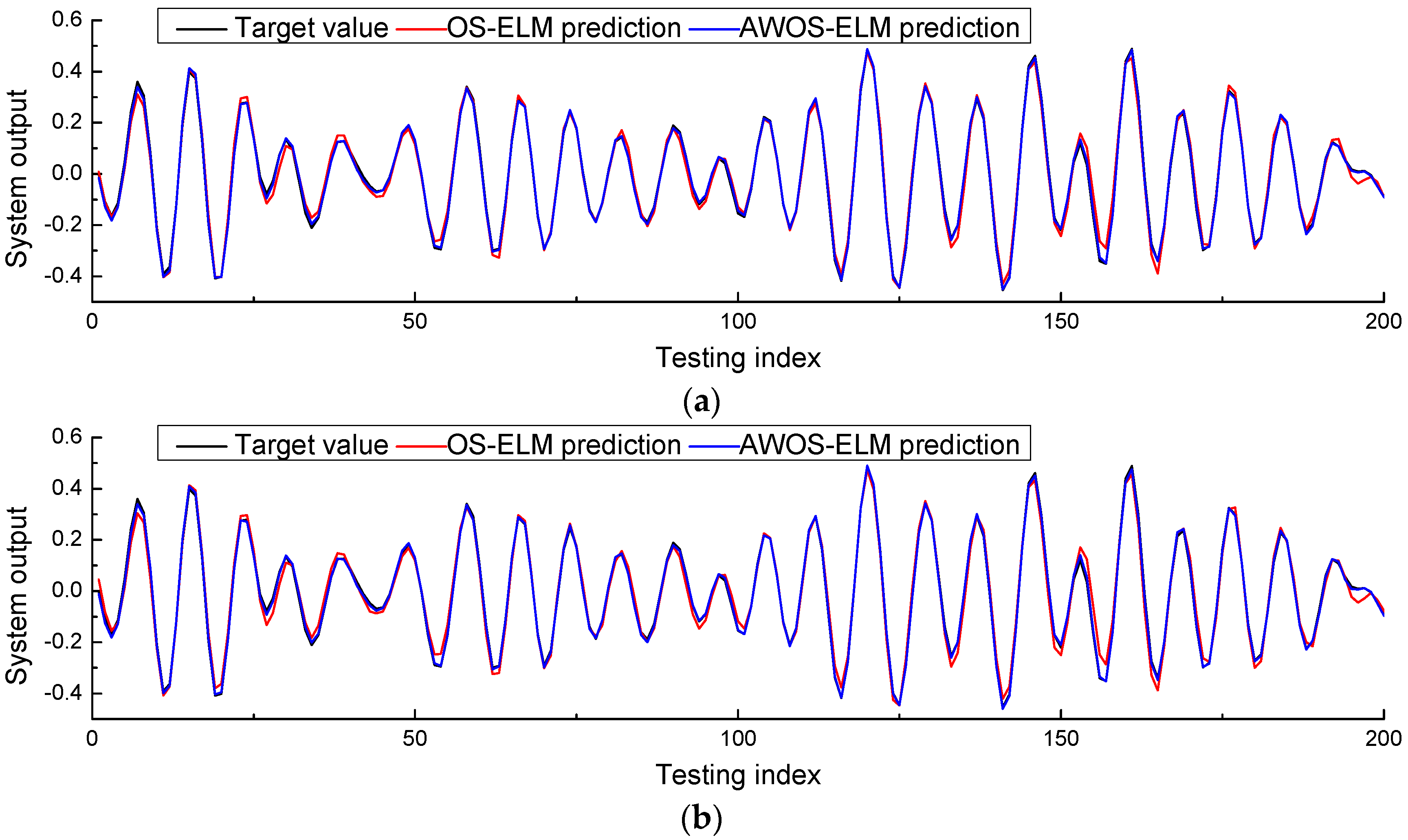
4.2. Robot Arm Example

In this subsection, the performance of AWOS-ELM and OS-ELM are compared on the identification problem regarding the dynamics modeling of a robot arm. The system input and output of this flexible robot arm are the measured reaction torque and the acceleration, respectively [27]. There are two attributes in this flexible robot arm example, and all of the 1024 pairs of data are described in Figure 2. In order to learn the model, the input and output of SLFN, $x_i$ and $t_i$, are respectively defined as $x_i={\left[u_i,u_{i-1},u_{i-2},u_{i-3},u_{i-4},d_{i-1},d_{i-2},d_{i-3},d_{i-4}\right]}^T$ and $t_i=d_i$, where $u_i$ and $d_i$ are the measured reaction torque and the acceleration of this robot arm, respectively. Thus, the samples number is 1019. The training set contains the front 819 samples, and the rest of the 200 samples are used to test the network.

Figure 3 illustrates the relationship between the hidden nodes number and testing RMSE of the OS-ELM and AWOS-ELM algorithms. It shows that the OS-ELM and AWOS-ELM with low hidden nodes number have similar testing RMSE, and the testing RMSE of AWOS-ELM algorithm tends to be lower than that of OS-ELM when the hidden nodes number increases. It shows that the OS-ELM and AWOS-ELM with low hidden nodes number have similar testing RMSE, and the testing RMSE of the AWOS-ELM algorithm tends to be lower than that of OS-ELM when the hidden nodes number increases. When the number of hidden nodes is too small, the prediction accuracy of SLFN trained by the OS-ELM or AWOS-ELM algorithm is very low. As described in Equations (17) and (18), the computing adaptive weight depends on the prediction value. If the prediction accuracy is too low, the AWOS-ELM cannot differentiate the low confidence data and normal data very well. Thus, in Figure 3, the performance of AWOS-ELM is similar to or even slightly less than that of OS-ELM when the hidden node number is low. In order to be fair for the sake of comparison, the hidden nodes number is set to be 45, which can guarantee that the algorithms with sigmoid function or RBF function both have fine performance levels. Figure 4 illustrates the identification effectiveness of the flexible robot arm dynamics modeling problem, and we can easily find that the AWOS-ELM algorithm has higher prediction accuracy than OS-ELM algorithm no matter whether considering the sigmoid function case or RBF function case.

Table 3. Performance comparison between AWOS-ELM and OS-ELM on the robot arm example.

Hidden Node Type	Algorithms	RMSE	$\mathit{\sigma }$	Hidden Nodes Number	${\mathit{\tau }}_{\mathit{r}}$	Chunk Size	Training Time/s
Sigmoid function	OS-ELM	0.0207	0.0004	45	-	5	0.1401
	AWOS-ELM	0.0081	0.0004	45	0.04	5	0.1426
Radial basis function	OS-ELM	0.0198	0.0006	45	-	5	0.3738
	AWOS-ELM	0.0084	0.0007	45	0.04	5	0.4115

showcases that the proposed AWOS-ELM algorithm and OS-ELM algorithm have similar training time and standard deviation values, implying the similar learning speed and stability, and that the AWOS-ELM algorithm has lower RMSE than the OS-ELM algorithm, which implies better generalization performance and higher prediction accuracy.

5. Conclusions

In lots of online learning applications, the sequentially arrived data usually have varying confidence coefficients. OS-ELM trains the neural network chunk-by-chunk, but at the same time, it cannot deal with varying confidence coefficients of each data chunk very well. Based on the OS-ELM algorithm, we propose a novel algorithm, AWOS-ELM, which assesses the confidence coefficient and determines the weight of each data chunk before using the chunk to train the network. The proposed AWOS-ELM algorithm can improve the learning process by picking out the abnormal samples which may mislead the subsequent learning process, thereby reducing the impact of these abnormal samples. Thus, the AWOS-ELM is able to learn sequentially similar to how the OS-ELM works, but at the same time deals with the varying confidence coefficients of each data chunk properly. Compared with OS-ELM, simulations on benchmark databases demonstrate that AWOS-LEM performs better in generalization performance, stability, and prediction accuracy. In addition, experimental results on a flexible robot arm identification problem demonstrate that AWOS-ELM has the ability to get higher prediction accuracy than OS-ELM, while the two algorithms have similar training speed and stability.

References

1. Shukla, A.K.; Garde, Y.A.; Jain, I. Forecast of Weather Parameters Using Time Series Data. MAUSAM 2014, 65, 209–520. [Google Scholar]
2. Kato, R.; Nagao, T. Stock Market Prediction Based On Interrelated Time Series Data. In Proceedings of the IEEE Symposium on Computers & Informatics, Penang, Malaysia, 18–20 March 2012.
3. Soni, S.K.; Chand, N.; Singh, D.P. Reducing the Data Transmission in WSNs Using Time Series Prediction Model. In Proceedings of the IEEE International Conference on Signal Processing, Communications and Computing, Hong Kong, China, 13–15 August 2012.
4. Hulsmann, M.; Borscheid, D.; Friedrich, C.M.; Reith, D. General Sales Forecast Models for Automobile Markets and Their Analysis. Trans. Mach. Learn. Data Min. 2011, 5, 65–86. [Google Scholar]
5. Gooijer, J.G.D.; Hyndman, R.J. 25 Years of Time Series Forecasting. Int. J. Forecast. 2006, 22, 443–473. [Google Scholar] [CrossRef]
6. Box, G.E.P.; Jenkins, S.B. Time Series Analysis: Forecasting and Control. J. Oper. Res. Soc. 1976, 22, 199–201. [Google Scholar]
7. Smith, C.; Jin, Y. Evolutionary Multi-objective Generation of Recurrent Neural Network Ensembles for Time Series Prediction. Neurocomputing 2014, 143, 302–311. [Google Scholar] [CrossRef] [Green Version]
8. Donmanska, D.; Wojtylak, M. Application of Fuzzy Time Series Models for Forecasting Pollution Concentrations. Expert Syst. Appl. 2012, 39, 7673–7679. [Google Scholar] [CrossRef]
9. Kumar, N.; Jha, G.K. A Time Series ANN Approach for Weather Forecasting. Int. J. Control Theory Comput. Model 2013, 3, 19–25. [Google Scholar] [CrossRef]
10. Claveria, O.; Torra, S. Forecasting Tourism Demand to Catalonia: Neural Networks vs. Time Series Models. Econ. Model 2014, 36, 220–228. [Google Scholar] [CrossRef] [Green Version]
11. Flores, J.J.; Graff, M.; Rodriguez, H. Evolutive Design of ARMA and ANN Models for Time Series Forecasting. Renew. Energ. 2012, 44, 225–230. [Google Scholar] [CrossRef]
12. Adhikari, R. A Neural Network Based Linear Ensemble Framework for Time Series Forecasting. Neurocomputing 2015, 157, 231–242. [Google Scholar] [CrossRef]
13. Kumar, D.A.; Murugan, S. Performance Analysis of Indian Stock Market Index Using Neural Network Time Series Model. In Proceedings of the International Conference on Pattern Recognition, Informatics and Mobile Engineering, Salem, India, 21–22 February 2013.
14. Yoon, H.; Hyun, Y.; Ha, K.; Lee, K.; Kim, G. A Method to Improve the Stability and Accuracy of ANN- and SVM-Based Time Series Models For Long-Term Groundwater Level Predictions. Comput. Geosci. 2016, 90, 144–155. [Google Scholar] [CrossRef]
15. Huang, G.B.; Chen, L.; Siew, C.K. Universal Approximation Using Incremental Constructive Feedforward Networks with Random Hidden Nodes. IEEE T. Neural Netw. 2006, 17, 879–892. [Google Scholar] [CrossRef] [PubMed]
16. Huang, G.B.; Zhu, Q.Y.; Siew, C.K. Extreme Learning Machine: A New Learning Scheme of Feedforward Neural Networks. In Proceedings of the International Joint Conference on Neural Networks, Budapest, Hungary, 25–29 July 2004.
17. Huang, G.B.; Zhu, Q.Y.; Siew, C.K. Extreme Learning Machine: Theory and Applications. Neurocomputing. 2006, 70, 489–501. [Google Scholar] [CrossRef]
18. Hosseinioun, N. Forecasting Outlier Occurrence in Stock Market Time Series Based on Wavelet Transform and Adaptive ELM Algorithm. J. Math. Financ. 2016, 6, 127–133. [Google Scholar] [CrossRef]
19. Dash, R.; Dash, P.K.; Bisoi, R. A Self Adaptive Differential Harmony Search Based Optimized Extreme Learning Machine for Financial Time Series Prediction. Swarm Evol. Comput. 2014, 19, 25–42. [Google Scholar] [CrossRef]
20. Liang, N.Y.; Huang, G.B.; Saratchandran, P.; Sundararajan, N. A Fast and Accurate Online Sequential Learning Algorithm for Feedforward Networks. IEEE T. Neural Netw. 2006, 17, 1411–1423. [Google Scholar] [CrossRef] [PubMed]
21. Huang, G.B.; Zhou, H.M.; Ding, X.J.; Zhang, R. Extreme Learning Machine for Regression and Multiclass Classification. IEEE Trans. Syst. Man Cybern. B 2012, 42, 513–529. [Google Scholar] [CrossRef] [PubMed]
22. Huang, G.; Ding, X.; Zhou, H. Optimization Method Based Extreme Learning Machine for Classification. Neurocomputing. 2010, 74, 155–163. [Google Scholar] [CrossRef]
23. Deng, C.Y. A Generalization of the Sherman-Morrison-Woodbury Formula. Appl. Math. Lett. 2011, 24, 1561–1564. [Google Scholar] [CrossRef]
24. Guo, W.; Xu, T.; Tang, K. M-Estimator-Based Online Sequential Extreme Learning Machine For Predicting Chaotic Time Series with Outliers. Neural Comput. Appl. 2016, 2016, 1–18. [Google Scholar] [CrossRef]
25. EI-Sayed, A.M.; Salman, S.M.; Elabd, N.A. On a Fractional-Order Delay Mackey-Glass Equation. Adv. Differ. Equ. 2016, 2016, 1–11. [Google Scholar]
26. Berezowski, M.; Grabski, A. Chaotic and Non-chaotic Mixed Oscillations in a Logistic Systems with Delay. Chaos Solitons Fractals 2002, 14, 1–6. [Google Scholar] [CrossRef]
27. Balasundaram, S.; Kapil, D.G. Lagrangian Support Vector Regression via Unconstrained Convex Minimization. Neural Net. 2014, 51, 67–79. [Google Scholar] [CrossRef] [PubMed]
Figure 1. Block diagram of the adaptive weight online sequential extreme learning machine (AWOS-ELM) algorithm.
Applsci 07 00217 g001
Figure 2. Flexible robot arm attributes. (a) System input; (b) system output.
Applsci 07 00217 g002
Figure 3. Relationship between testing RMSE and hidden nodes number. (a) Sigmoid node; (b) RBF node.
Applsci 07 00217 g003
Figure 4. Comparison of the prediction ability of the OS-ELM algorithm and the AWOS-ELM algorithm. (a) Sigmoid function; (b) RBF function.
Applsci 07 00217 g004