Predictive Modelling and Analysis of Process Parameters on Material Removal Characteristics in Abrasive Belt Grinding Process

Abstract

The surface finishing and stock removal of complicated geometries is the principal objective for grinding with compliant abrasive tools. To understand and achieve optimum material removal in a tertiary finishing process such as Abrasive Belt Grinding, it is essential to look in more detail at the process parameters/variables that affect the stock removal rate. The process variables involved in a belt grinding process include the grit and abrasive type of grinding belt, belt speed, contact wheel hardness, serration, and grinding force. Changing these process variables will affect the performance of the process. The literature survey on belt grinding shows certain limited understanding of material removal on the process variables. Experimental trials were conducted based on the Taguchi Method to evaluate the influence of individual and interactive process variables. Analysis of variance (ANOVA) was employed to investigate the belt grinding characteristics on material removal. This research work describes a systematic approach to optimise process parameters to achieve the desired stock removal in a compliant Abrasive Belt Grinding process. Experimental study showed that the removed material from a surface due to the belt grinding process has a non-linear relationship with the process variables. In this paper, the Adaptive Neuro-Fuzzy Inference System (ANFIS) model is used to determine material removal. Compared with the experimental results, the model accurately predicts the stock removal. With further verification of the empirical model, a better understanding of the grinding parameters involved in material removal, particularly the influence of the individual process variables and their interaction, can be obtained.

1. Introduction

Abrasive grinding is a widely employed finishing process, with abrasive grains being used as the cutting edge to accomplish close tolerances and excellent dimensional correctness and surface integrity. Abrasive Belt Grinding is a modification of the traditional grinding processes in which the contact wheel is made of polymer backing material. The grinding belt is formed of abrasives coated on a backing material and fastened around at least two rotating polymer contact wheels, which make it a compliant tool, as shown in Figure 1. The soft contact polymer wheel enables this machining process to be appropriate to machine free-form surfaces due to its versatility, efficiency, and ability to machine workpieces of intricate shapes and geometry [1]. Understanding of such a process is one of the most delicate problems in the industry due to the high complexity and nonlinearity. The process parameters affecting material removal belt grinding are that the complex and non-linear behaviour of the belt grinding tool is predominantly dependent on the contacts amid the workpiece and abrasive belt. Jourani et al. [2] have presented a three-dimensional numerical model, which could determine pressure distribution along with the distribution of real contact to study the contact between the belt constituted by abrasive grains and the surface to understand the material removal mechanism. Zhang et al. [1] have stated that force distribution in the contact area between the workpiece and the elastic contact wheel determines the ratio of material removal in the belt grinding process. Ren et al. [3,4] developed a local process model to predict the material removal rate before machining, making it suiT for the robot programmer to optimize the tool path based on simulation results. Hamann [5] had proposed a linear mathematical model for material removal based on cutting parameters. However, the proposed equation is no longer adequate for intricate surfaces, as both complete removal and local removals are not equivalently distributed in the entire contact area due to the complex geometry of the workpiece that is machined. According to the brief literature review above, it can be concluded that most of the previous research works concentrated on cutting path optimization, thereby making regular contact resulting in constant material removal [6,7,8,9]. Though the removal of material in the belt grinding process from the workpiece surface can be written as a function of several parameters, their influence and interaction have not been reported in the literature that will be covered and bridged in this research work. The material removal volume depends mainly on the contact force between the tool and the workpiece, the belt speed, and the feed rate in the tangential direction. The influences of these parameters on the material removal rate were examined experimentally. Orthogonal arrays of Taguchi, analysis of variance (ANOVA), and regression analyses are employed to analyse the effect of the belt grinding parameters on the depth of cut, i.e., metal removal rate. The Taguchi Method uses orthogonal arrays in experimental design for a significant reduction in the number of experimental runs to find the optimal solution. Taguchi methods have been widely utilised in engineering analysis to obtain information about the behaviour of a given process [10]. ANOVA is a statistical based analysis employed to indicate the impact of process parameters on the process output and helps in predicting the significance of all factors and their interactions [11]. In this research, we have also proposed a numerical model to predict material removal as a function of process parameters, namely, hardness, force, rotation speed, grit size, and feed rate, based on the Adaptive Neuro-Fuzzy Inference System (ANFIS). The ANFIS technique has been used in the past for the prediction and modelling of material removal as a function of the process parameters [12,13]. The Adaptive Neuro-Fuzzy Inference System (ANFIS) conjoins the benefits of the neural network and fuzzy systems [14]. When experimental data and model results are compared, it is observed that the developed regression model is within the limits of the acceptable error.

The paper is organised as follows; a brief overview of the Abrasive Belt Grinding process and the problem statement is presented in Section 1, followed by a brief outline of the belt grinding process and the Adaptive Neuro-fuzzy Inference System (ANFIS) in Section 2. The machining conditions, experimental setup, process parameter and the Taguchi orthogonal array design to minimise the number of grinding experiments are reported in Section 3. The results of the belt grinding tests are analysed using the signal to noise ratio (S/N) and ANOVA in Section 4, followed by a summary of the predictive modelling of material removal using ANFIS. Finally, the conclusions of this research work are reviewed in Section 5.

2. Theoretical Basis

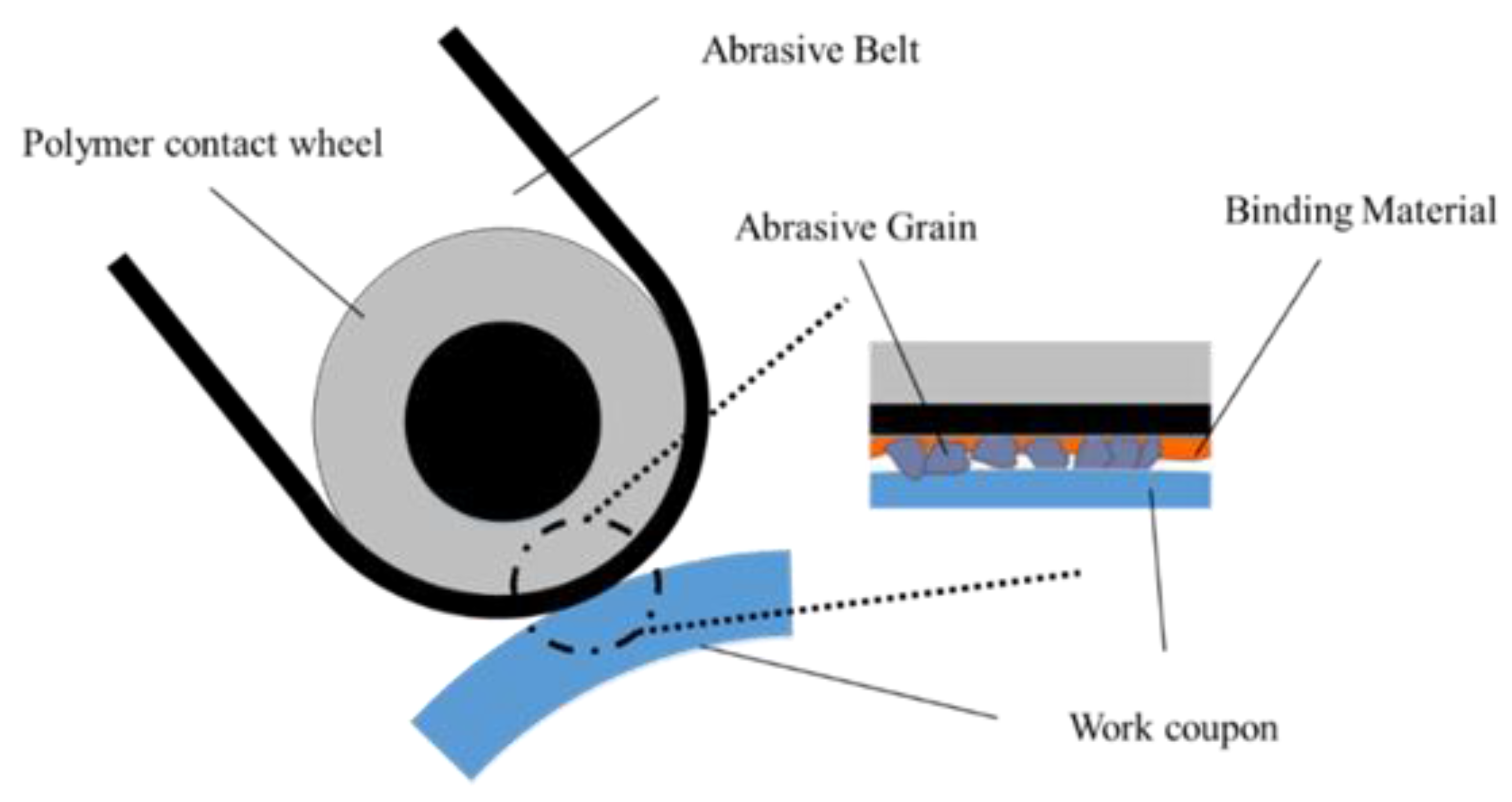
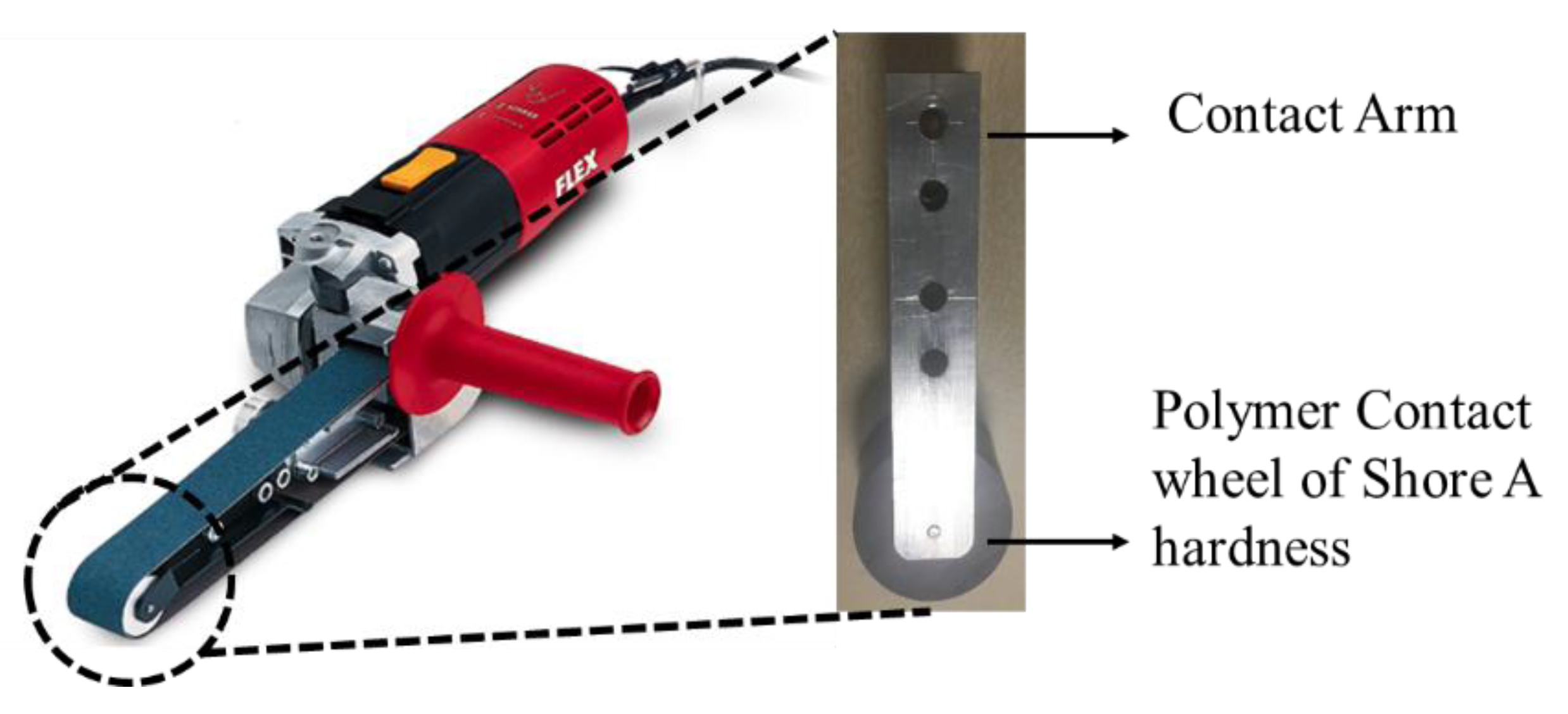
2.1. Abrasive Belt Grinding Process

Abrasive Belt Grinding is a tertiary polishing process with a geometrically indeterminate machining edge with multiple grains. The belt grinding setup has an elastic contact roller wheel made up of thermosetting polyurethane elastomer, which can be deformed to assist the coated abrasive belt that functions as the cutting edge, as illustrated in Figure 1. Compliant belt grinding corresponds to elastic grinding and has the capabilities of grinding, milling, and polishing [15].

The belt grinding process has characteristics of good workpiece-shape adaptability with uniform material removal, low grinding temperature, maintenance of residual compressive stresses, and resistance to workpiece burning like any other tertiary finishing process. The belt grinding process can quickly generate surfaces with high levels of precision and smoothness. Presently, about one-third of abrasive wheel grinding has been substituted by belt grinding [15]. Similar to any other abrasive machining process, many process parameters in belt grinding impact the last ground surface quality, including the grinding belt topography features and cutting parameters. The process parameters include belt speed, belt preloaded tension, the force imparted, feed rate, workpiece geometry, polymer hardness, and belt topography features such as grit size [3]. Hamann [5] had proposed a linear mathematical model as shown below as Equation (1), which states that the overall material removal rate (MRR) r is either relative or inversely proportional to parameters such as C_A (constant of the grinding process), K_A (combination constant of resistance factor of the work coupon and grinding ability factor of the belt), k_t (belt wear factor), V_b (grinding rate), V_w (feed-in rate), L_w (machining width), and F_A (normal force).

$$r=C_A.K_A.k_t.\frac{V_b}{V_w.L_w}.F_A$$

(1)

The material removal intensifies when the number of the interactions of the abrasive grains per unit time gets maximised [16]. Therefore it is evident that material removal is directly proportional to the cutting speed (grinding rate) of the polymer contact wheel on the belt grinder. The depth of penetration depends on the topography and the geometry of the belt/wheel surfaces, which serves as an undefined cutting-edge. The coarser grain sizes exhibit a greater ability to achieve higher cutting depth, which results in higher material removal than finer sizes. Material removal increases with a higher dwell time of interaction between the cutting grain edges, and workpiece surface, i.e., material removal, is inversely proportional to the feed-in rate [16]. Adequate force is required for the cutting edge to penetrate deeply into the workpiece to achieve grain cutting depth resulting in material removal. The penetration depth of the grains into the work coupon surface predominantly depends on the force imparted for grinding [16]. Belt finishing with contact wheels of different hardnesses results in dynamic changes in contact pressure, leading to a change in the mechanism of wear. This hints that the parameters discussed govern the belt grinding process, and changing any of the parameters will have a resultant shift in the output. Stock removal commonly requires a harder polymer contact wheel, coarse abrasive grains, greater force, reduced feed, and better cutting speed. Finishing requires the use of a softer contact wheel and fine grade abrasive grains. However, the degree of the effect will vary parameter to parameter. The amount of material removed from the workpiece surface results from the distinct local contact conditions, which are completely influenced by the process parameters/variables. The relationship between the material removal rate and process parameters is not well grasped, even though machining by belt grinding is remarkably straightforward and inexpensive. Belt grinding is used in industries based on operator’s skill and knowledge, making the process inherently exhibit poor stability and reproducibility.

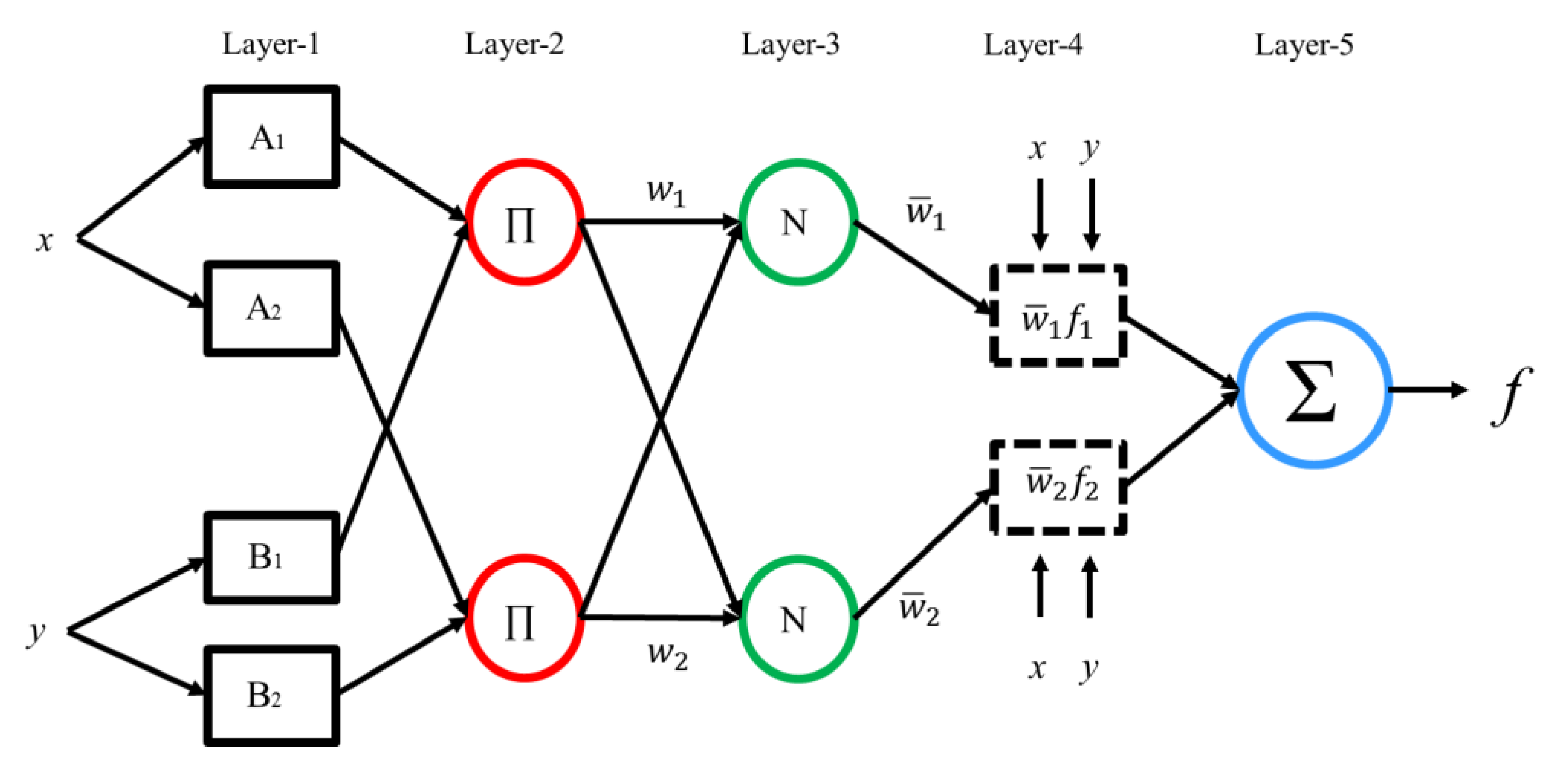
2.2. Adaptive Neuro-Fuzzy Inference System

The Adaptive Neuro-Fuzzy Inference System (ANFIS) is a blend of the neural network and fuzzy inference system. Fuzzy inference systems have no learning capabilities regarding the input-output space and no standard tuning methods for their rule bases, which make system adaptations difficult. The ANFIS technique offered a method for the fuzzy systems to acquire knowledge regarding the dataset to calculate the membership function parameters that permitted Fuzzy Inference System (FIS) for automatic system adaption. ANFIS architecture is a superimposition of FIS on the Artificial Neural Network (ANN) architecture, which will enable FIS to optimise its rule base based on the output to learn like an ANN eliminating its inherent disadvantage. The ANFIS algorithm has an in-built advantage compared to fuzzy models as it holds the learning competencies of the ANN, which augments the system performance using a priori understanding [17]. Using an input and output space relation, ANFIS forms an FIS, the membership function of which is altered by exploiting the back-propagation algorithm and least square method available with ANN [18].

In this section, the ANFIS architecture and its learning algorithm for the Sugeno fuzzy model will be described primarily. The ANFIS architecture is shown in Figure 2; ANFIS normally has five layers of neurons, of which neurons in the same layer are of the same function family. Assume that the FIS under consideration has two inputs, x and y, which form two fuzzy if–then rules based on first-order Sugeno fuzzy model [19].

• Rule 1: If x is A1 and y is B1, then f1 = p1x +q1y + r1;
• Rule 2: If x is A2 and y is B2, then f2 = p2x +q2y + r2;
• where p1, p2, q1, q2, r1, and r2 are linear parameters and A1, A2, B1, and B2 are nonlinear parameters. The output of the ith node in layer 1 is denoted as O_l,i.
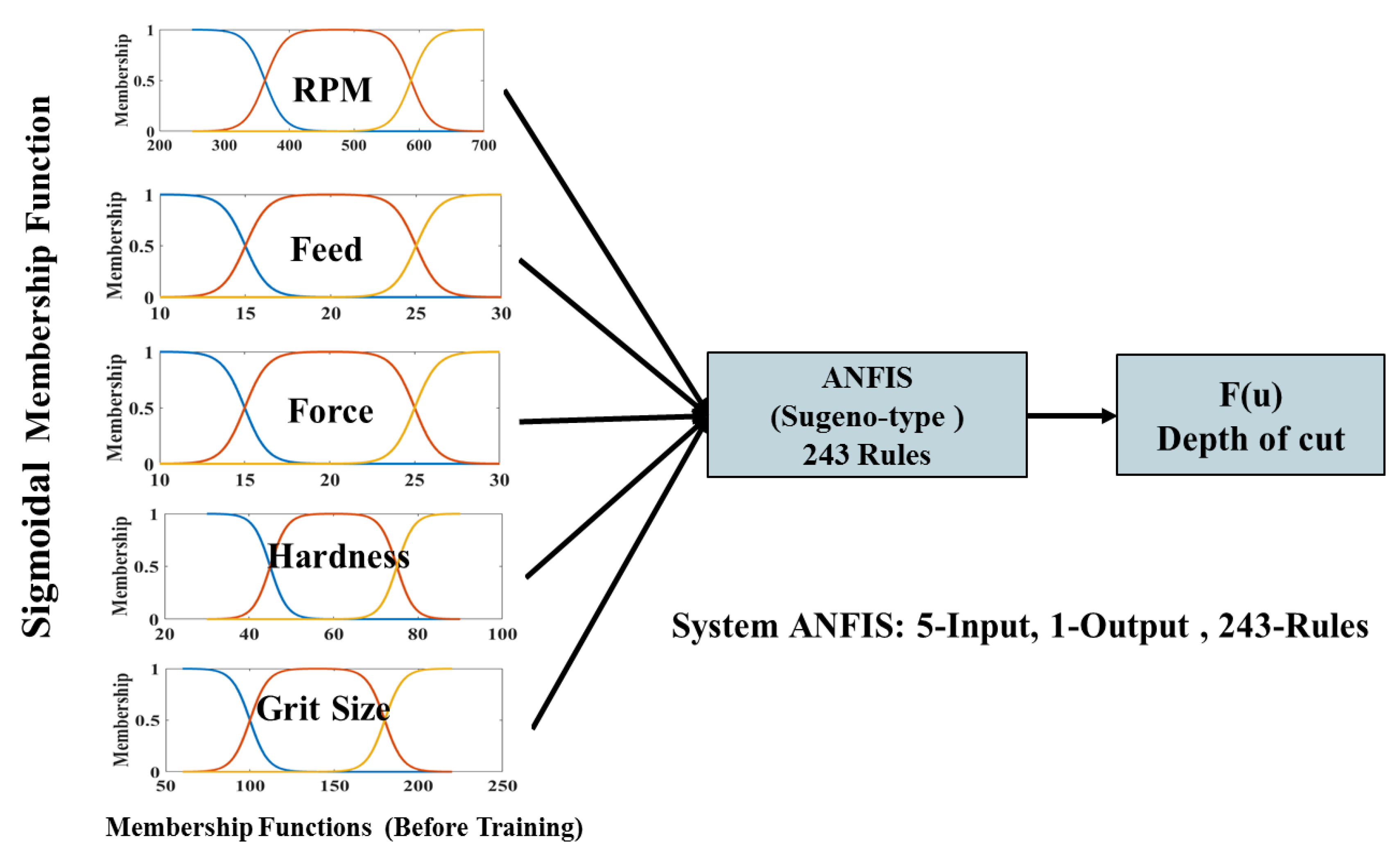
• Layer 1: Every adaptive node i in the layer 1 has a node function.

  $$O_{l,i}={\mu }_{A_i}\left(x\right)fori=1,2,or O_{l,i}={\mu }_{B_{i-2}}\left(y\right)fori=3,4$$

  (2)

  where x (or y) is the input to nodes i and A_i (or B_i–2) generating a linguistic label coupled with the node as given by Equation (2). The membership function for A (or B) can be any, parameterized as a sigmoidal membership function given by Equation (3).

  $${\mu }_{A_i}\left(x\right)=\frac{1}{1+e^{-a\left(x-c\right)}}$$

  (3)

  where (c_i, a_i) is the parameter set. These are called premise parameters. As the values of the parameters change, the shape of the membership function varies.
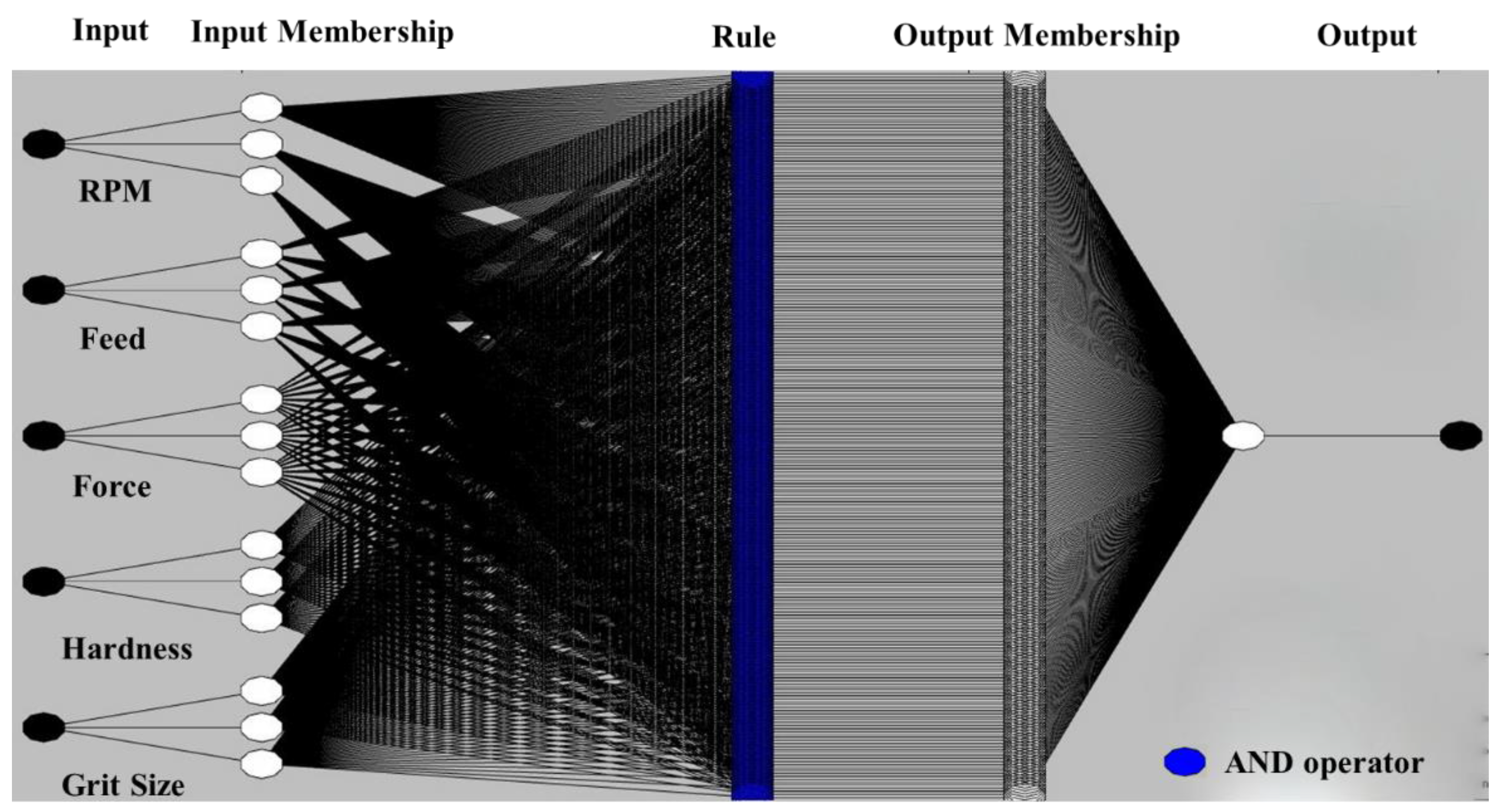
• Layer 2: Every node in layer 2 is a fixed node labelled ∏. Each node calculates the firing strength of each rule, which is the output using the simple product operator. Evaluating the rule premises results as a product of all of the incoming signals given by Equation (4)

  $$O_{2,i}=w_i={\mu }_{A_i}\left(\mathrm{x}\right)\times {\mu }_{B_i}\left(y\right)fori=1,2$$

  (4)
• Layer 3: The ratio of the ith rule’s firing strength to the sum of all of the rule’s firing strengths is calculated by Equation (5) in layer 3. The output of this layer is called normalized firing strengths.

  $$O_{3,i}={\overline{w}}_i=\frac{w_i}{{\mathsf{\Sigma }}_i^2{w}_i}=\frac{w_i}{w_1+w_2}i=1,2$$

  (5)
• Layer 4: Every node i in layer 4 is an adaptive node with a node function. The nodes compute a parameter function on the layer output. Parameters in this layer will be referred to as consequent parameters.

  $$O_{4,i}={\overline{w}}_i{f}_i={\overline{w}}_i\left(p_{i}x+q_{i}y+r_i\right)$$

  (6)

  where w_i is a normalised firing strength from layer 3 and (p_i, q_i, r_i) is the parameter set for the node.
• Layer 5: This layer has a fixed single node labelled Σ, which computes the overall output as the summation of all of the incoming signals, as shown in Equation (7). The Σ gives the overall output of the constructed adaptive network, having same functionality as the Sugeno fuzzy model.

  $$O_{5,i}={\displaystyle \sum }_i{\overline{w}}_i{f}_i=\frac{{{\displaystyle \sum }}_i{w}_i{f}_i}{{{\displaystyle \sum }}_i{w}_i}$$

  (7)

From Figure 2, it can be noticed that the input membership functions of the Takagi-Sugeno model are non-linear, whereas the output membership functions are linear.

3. Experimental Procedures

3.1. Experiment Design Based on Taguchi Method

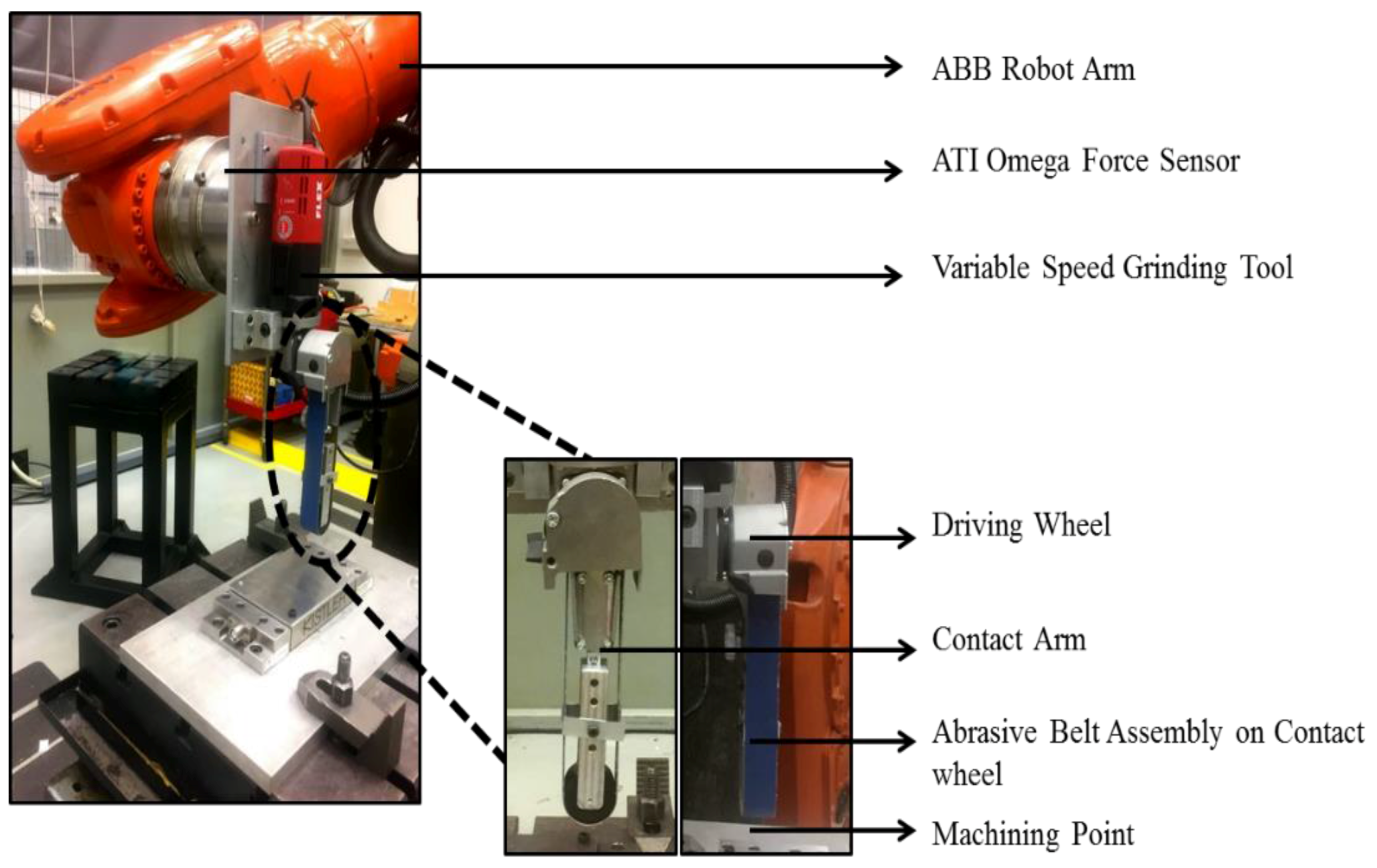
3.1.1. Experimental Setup

Belt grinding is a modification of the traditional grinding processes, with the contact wheel being made of compliant polymer material. The abrasive belt sander, as shown in Figure 3, is customised with a fixture design such that it can be used as a belt grinding tool. A belt sander is an electrically powered abrasive belt tool that can be run at different variable speeds at unloading conditions. Ester polyurethane polymer of different Shore A hardnesses is used as a contact wheel, which forms the part of the contact arm, which is used as the machining end of the custom belt grinder setup, as shown in Figure 3. The use of robots or multiple-axes machining centres improves the finishing efficiency.

The experimental trials were conducted on coupling the belt sander and an ABB 6660-205-193 multi-axes robot using a suitable fixture, as shown in Figure 4. The ABB 6660-205-193 has a parallel arm structure, powerful gears, and motors for handling fluctuating process forces prevalent within applications such as milling, deburring, and grinding. An ATI force sensor (Omega 160) connects the fixture and the robot arm end effector. This is accomplished by mounting the force sensor to the ABB robots end-effector and then attaching the customised belt grinding tool to the force sensor, as shown in Figure 4. The robot controller continuously receives the force/torque signal, compares it with the users input, and achieves force compensation. The system is close looped, and this ensures that the force programmed and the force exerted are the same. The robot arm is primarily used for toolpath control and force control.

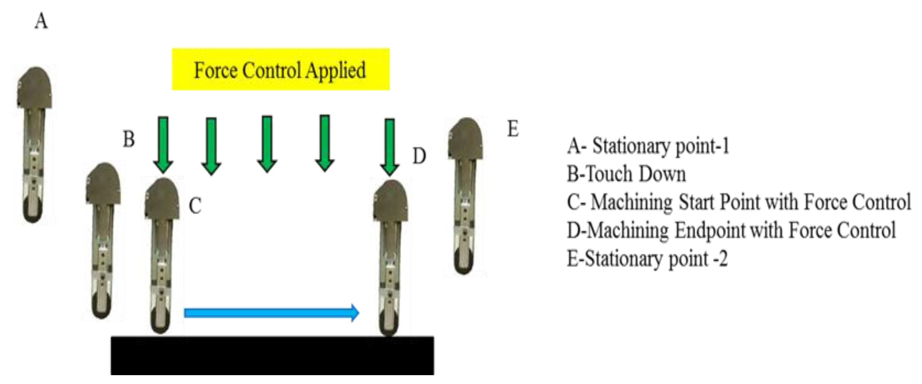
3.1.2. Toolpath Planning

Force control is essential for avoiding over and under-cutting of the material. Force control is particularly used for uniform material removal along the whole toolpath. Such an adaptive tool for path generation in the system was realised with (ATI Omega 160) force control in the experimental trials. A constant contact force throughout the abrasive belt finishing the process in the normal direction (Z-axis) is achieved by using a force sensor (ATI Omega 160) attached to the end effector of the robotic arm of an ABB 6660 robot. The force sensor maintains an adequate in-feed in the normal direction. Tool path planning has five different zones, as shown in Figure 5. Zone A and Zone B are when the abrasive belt tool enters the machining region, zone C is where the actual machining happens in force control mode, and zones D and E are where the abrasive belt tool exits the machining region. ABB Robot Studio executes tool path planning. Most of belt grinding processes are done on complicated geometries, and maintaining uniform material removal can be realised only when tool centre point (machining end) interacts with the surface normally, which is the current industrial practice employing highly automatic robotic arm manipulators.

3.1.3. Taguchi Based DoE (Design of Experiments)

As the knowledge of the likely interactions of the belt grinding parameters was not known initially, trials were planned using Taguchi orthogonal array design, showing only the effects of the individual parameters. To evaluate the effect of the belt grinding process parameters on material removal, Taguchi’s L27 orthogonal array (five-factor, three-level) model is selected, and experiments were performed based on it. In this study, the process parameters such as grit size, rubber shore A hardness, force, feed, and wheel speed are considered to analyse material removal.

Table 1. Belt grinding parameters and their levels.

Parameter	Unit	Levels
		L1	L2	L3
RPM	(m/min)	250	500	700
Feed	(mm/s)	10	20	30
Force	(N)	10	20	30
Rubber hardness	(Shore A)	30	60	90
Grit Size	-	60	120	220

shows a summary of process parameters and their level used for performing grinding trials. The experimental layout for the five cutting parameters using the L27 orthogonal array is provided in

Table 2. Taguchi Experimental design using the L27 orthogonal array and corresponding depth of cut and signal-to-noise (S/N) ratio.

Trial No.	Factors					MRR
	RPM	Feed	Force	Hardness	Grit	Depth of Cut	S/N Ratio
1	250	10	10	30	60	65.60076	36.338177
2	250	10	10	30	120	25.87109	28.256295
3	250	10	10	30	220	13.34471	22.506183
4	250	20	20	60	60	86.10453	38.70052
5	250	20	20	60	120	44.20156	32.908752
6	250	20	20	60	220	23.53456	27.434122
7	250	30	30	90	60	93.8753	39.451027
8	250	30	30	90	120	54.33391	34.701419
9	250	30	30	90	220	23.55062	27.440047
10	500	10	20	90	60	142.9324	43.102614
11	500	10	20	90	120	86.37583	38.727845
12	500	10	20	90	220	59.38035	35.472855
13	500	20	30	30	60	120.6638	41.63154
14	500	20	30	30	120	57.50747	35.194485
15	500	20	30	30	220	45.55799	33.171291
16	500	30	10	60	60	77.47286	37.782992
17	500	30	10	60	120	26.08495	28.3278
18	500	30	10	60	220	13.54166	22.633438
19	750	10	30	60	60	134.8952	42.59993
20	750	10	30	60	120	76.88529	37.716865
21	750	10	30	60	220	58.97687	35.413634
22	750	20	10	90	60	103.8255	40.326081
23	750	20	10	90	120	56.9663	35.11236
24	750	20	10	90	220	35.31606	30.959445
25	750	30	20	30	60	114.009	41.138783
26	750	30	20	30	120	56.65924	35.065415
27	750	30	20	30	220	44.31528	32.93107

. The mean S/N ratio for each level of the other machining parameters is assessed based on the material removal, i.e., depth of cut, and a greater S/N ratio corresponds to better material removal characteristics.

3.2. Experimental Conditions

The experimental studies were done on a belt grinding setup based on settings of machining parameters, which were defined by using the Taguchi experimental design method. In addition, the test conditions listed below were maintained constantly throughout to achieve a controlled experimental trial.

• The contact head of the belt grinder is kept at normal angle to keep uniformity in contact conditions throughout machining.
• Tool wear effect was ignored as the tests were conducted in the useful lifetime of the belt tool.
• The surface condition of the machined aluminium 6061 coupons was uniform with a surface roughness of 0.8 microns (μm).
• Experiments are carried out in dry conditions.
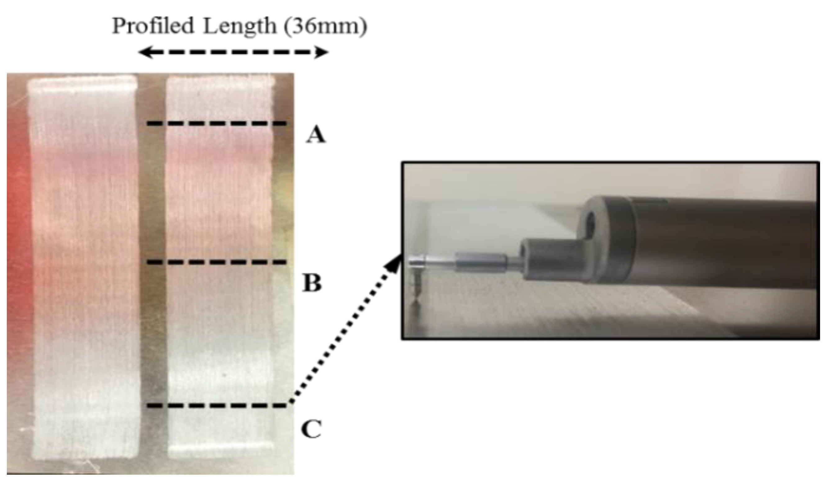
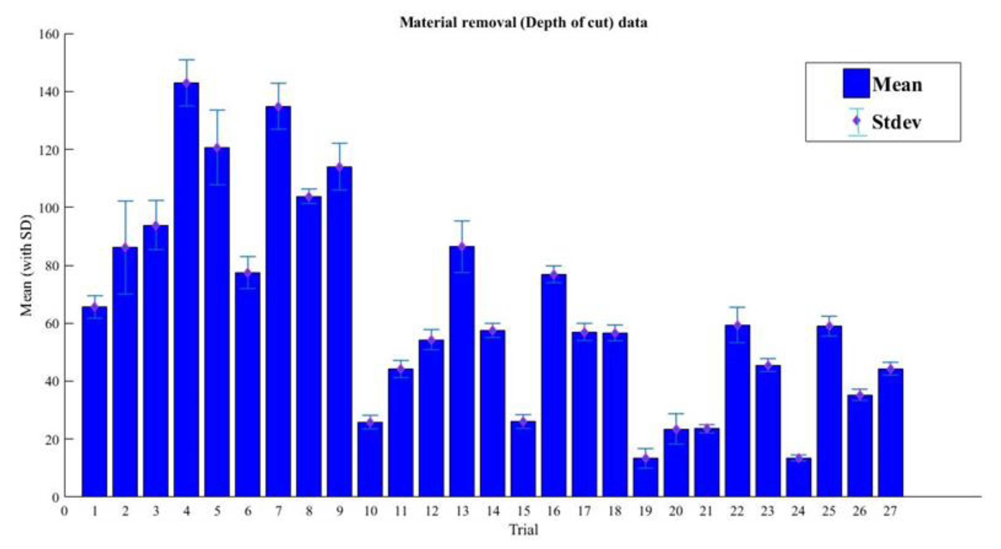
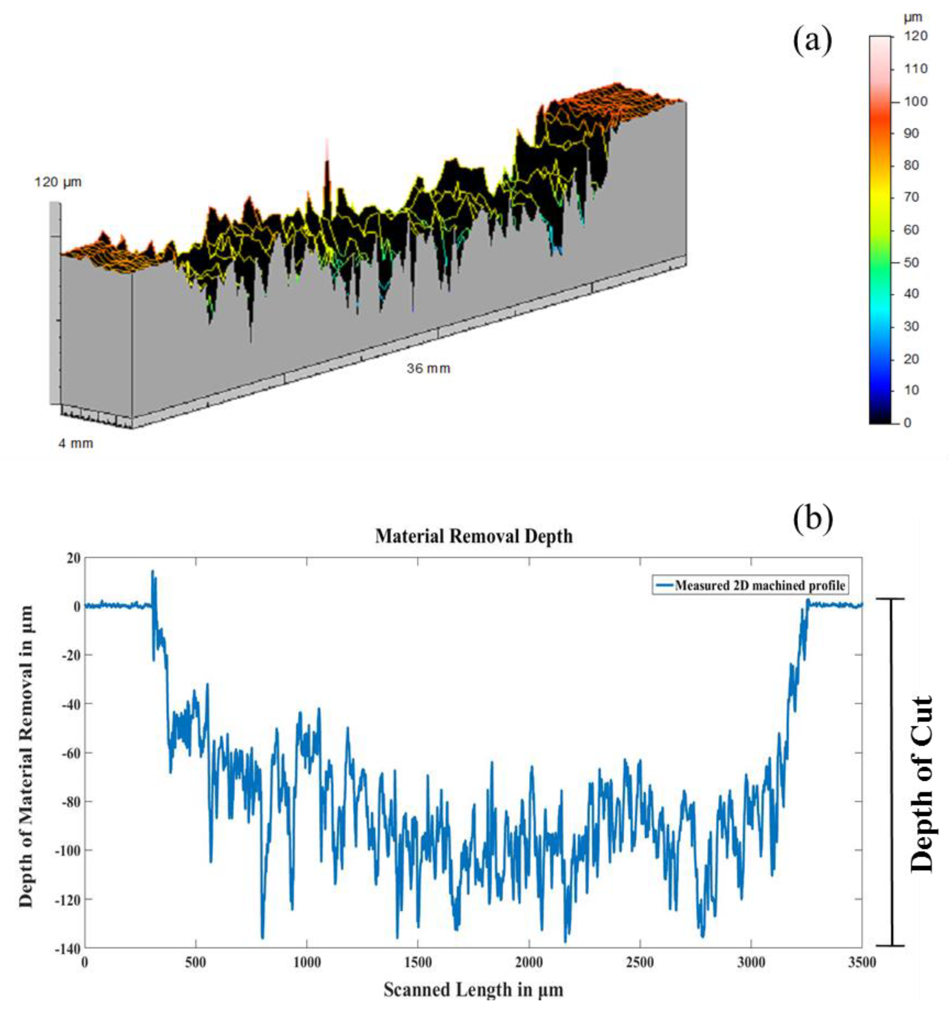
• Experiments were carried out with three passes for each trial. On each pass, the depth of cut was measured at three different locations, as shown in Figure 6, resulting in nine measurements. According to the parameter combinations from the Taguchi method, which obtained 27 trials as presented in Table 2, 243 depth of cut readings were obtained.

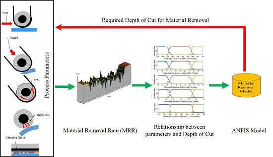
3.3. Prediction of Depth of Cut

A Mitutoyo stylus profilometer with a stylus tip radius of 5 µm was used to measure the depth of cut across the grinded path. Mitutoyo profilometer primarily consists of a traverse unit and a processor control module. The grinded workpieces are so adjusted that the area of interest of measurement is across the grinded path. The length is profiled across locations A, B, and C along the tool path, as shown in Figure 6. 3D and 2D profiles were extracted from the workpiece surface across the machined length, using the profilometer to measure the depth of cut, as illustrated in Figure 7.

The depth of cut is measured as the distance between the deepest point in the grinded path and the surface of the word coupon. Each experimental trial was repeated three times to have consistency, and depth of cut was measured across three locations for each trial, resulting in a total of nine reading per test. Figure 8 shows the standard deviation of the depth of cut measure taken from Taguchi’s L27 orthogonal array based experimental trials for all 27 test conditions. Table 2 shows the experimental results for the mean depth of cut and corresponding S/N ratios. The depth of cut, i.e., material removal, was identified as the process output as well as the quality characteristic with the concept ‘the larger-the-better’. The S/N ratio for the larger-the-better is: S/N = −10 × log (mean square deviation):

$$\frac{S}{N}=-10lo{g}_{10}\left(\frac{1}{n}{{\displaystyle \sum }}^{\text{}}\frac{1}{y^2}\right)$$

(8)

where n is the number of measurements in a trial/row, in this case, n = 1, and y is the measured value in a run/row. A higher S/N value agrees with a higher depth of cut. Consequently, the ideal level of the grinding parameters is the level with the most significant S/N value.

4. Results and Analysis

Figure 9 presents the results of the S/N ratio for the five parameters at three levels. According to Figure 9, the optimal parameters for a higher material removal rate were obtained at 750 RPM (level 3), 10 mm/s feed rate (level 1), 30 N force (level 3), 90 Shore A hardness (level 3), and 60 grit (level 1). The Material Removal Rate (MRR) increases with increasing Rotation per Minute (RPM), force, and hardness. On the contrary, it increases with decreasing feed and grit size. With coarser grain, i.e., smaller grit size, the depth of cut increases. An increase in force imparted on the work coupon and hardness of contact wheel results in an increase of material removal. The increase of RPM in the contact wheel causes greater tangential force, thereby causing the enhancement of the depth of cut. The decrease in feed rate causes the contact time between the grains and work coupon to be maximized, resulting in a higher material removal rate.

4.1. Analysis of Variance (ANOVA)

To understand a detailed visualisation of the impact of various factors influencing the depth of cut, i.e., material removal, in the belt grinding of Aluminium 6061 specimen, ANOVA was used. Based on the ANOVA, the comparative significance of the grinding parameters on the depth of cut was examined to define more accurately the optimum combination of the grinding parameters for higher material removal. The analysis is carried out for the level of significance of 5% (the level of confidence is 95%); the results are shown in

Table 3. Results of analysis of variance (ANOVA) for depth of cut.

Machining Parameter	Degrees of Freedom	Sum of Squares	Mean Square	F Ratio	Contribution (%)
RPM	2	5055.5	2527.7	26.42	13.54
Feed	2	1249.1	624.5	6.53	3.34
Force	2	4782.8	2391.4	25.00	12.79
Hardness	2	867.1	433.6	4.53	2.31
Grit	2	23,903.7	11,951.9	124.93	63.93
Error	16	1530.7	95.7	-	4.09
Total	26	37,388.8	-	-	-

. The last column of Table 3 shows the percentage impact of each parameter on the total variation, signifying their degree of effect on the results. The larger the percentage contribution, the greater the influence a parameter has on the material removal. It can be observed from Table 3 that the grit size (F = 124.93) has the greater static influence of 63.93%, followed by RPM (F = 26.42), which has an influence of 13.54%, and Force (F = 25.00), which has an influence of 12.79% on material removal rate. The feed and wheel hardnesses have an insignificant effect on the material removal of 3.34% and 2.31%.

Interaction plots are most often used to visualise interactions during ANOVA. The effect of one factor depends on the level of the other factor, and such possible interactions can be envisioned using an interaction plot. The two way interaction effects are shown as line plots in Figure 10. Figure 10, below, indicates the interaction plot among the five belt grinding parameters that have been considered in our study on the depth of cut.

4.2. Predictive Modelling of Material Removal Using ANFIS

Adaptive neuro-fuzzy inference system (ANFIS) removes the primary problem in fuzzy if-then rules by using the learning ability of an artificial neural network (ANN) for automated tuning of fuzzy if-then rules during training, resulting in a change of the membership function of parameters, thus leading to the automatic adaptation of the fuzzy system based on inputs-output space. The initial step of the ANFIS modelling system is to decide the input and output variables of the fuzzy logic controller. The ANFIS model described in this paper has five input parameters; RPM, feed, force, hardness, grit, and the output as the depth of cut, i.e., material removal rate (MRR).

The ANFIS model described in this paper is a Multiple Input Single Output (MISO) system with multiple inputs and a single output. Figure 11 shows real inputs and real output with fuzzy rule architecture of the ANFIS. A Taguchi based experimental design with 27 runs, as indicated in Table 2, is used as the inputs for the ANFIS model.

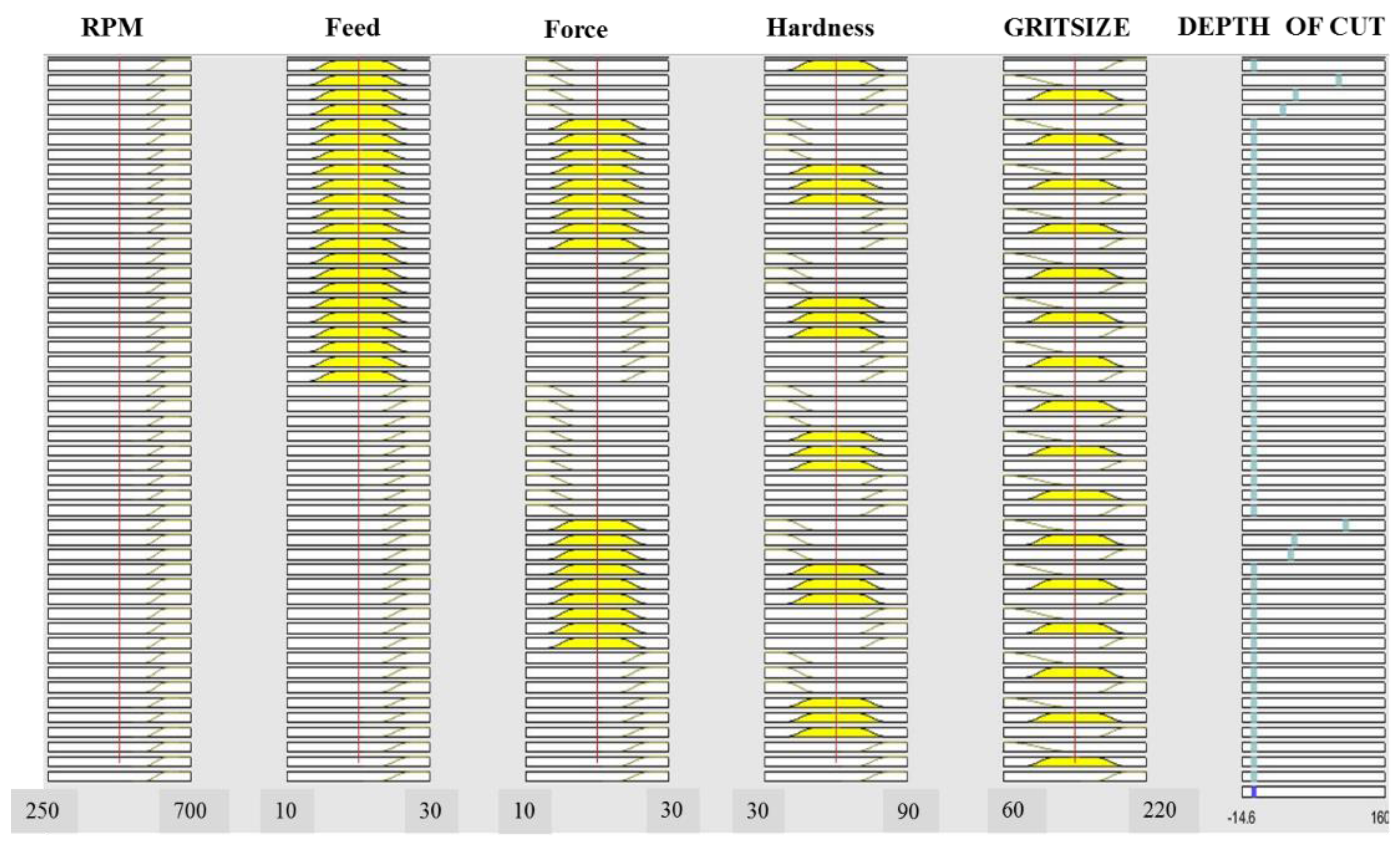
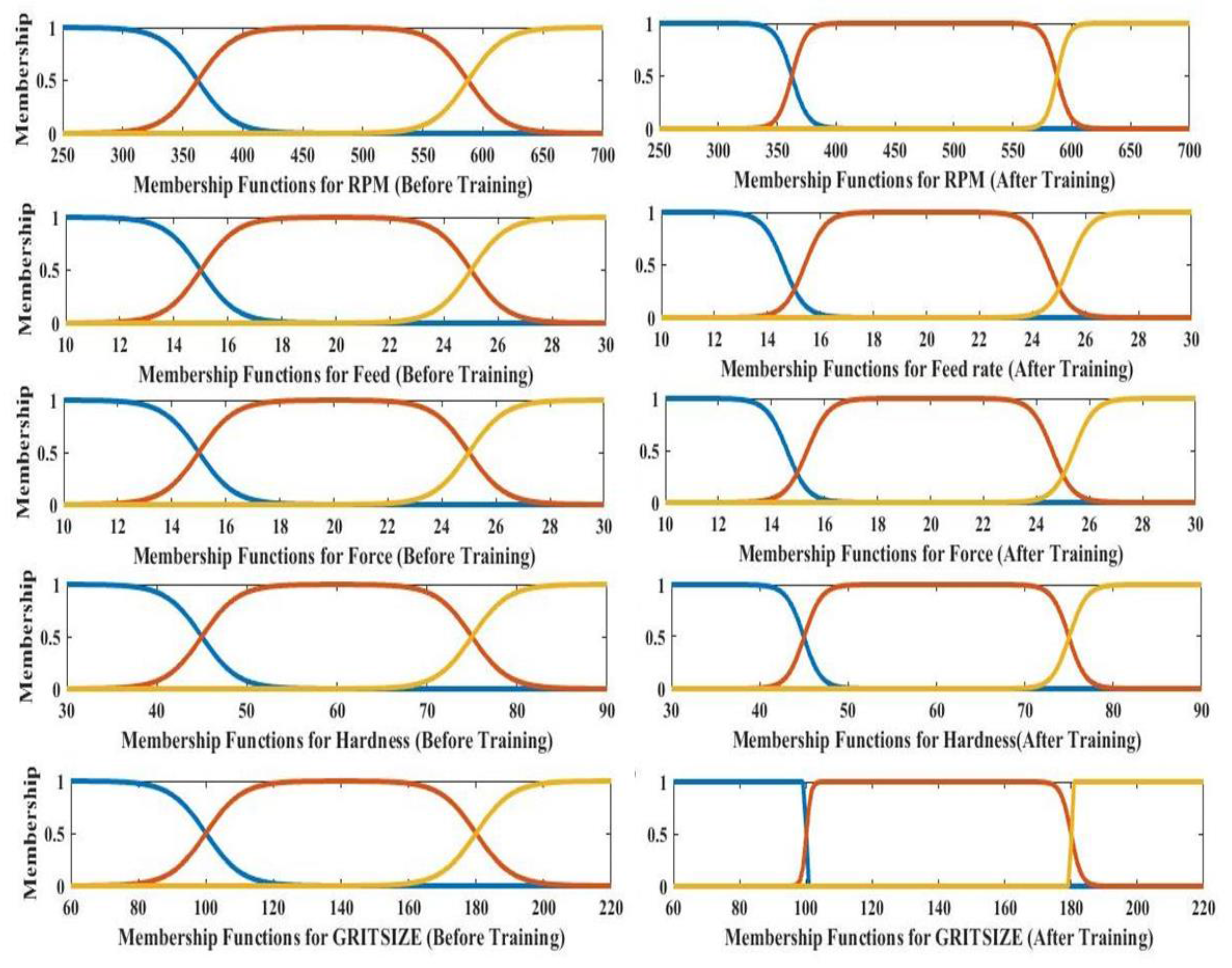
4.2.1. Membership Functions for the Input and Output Variables

A membership function allocates grades of membership extending from numbers between zero and one to the range of the possible values of the variable. Zero membership value specifies that it is not a member of the fuzzy-set; one signifies an extensive member. A membership function such as sigmoidal membership function is created for each input variable used in belt grinding, as illustrated in Figure 11. The sigmoid function is differentiable for all values of the inputs to allow the use of powerful back-propagation learning algorithms [20]. The application of general sigmoidal membership functions to the neuro-fuzzy modelling process is a very attractive methodology to characterise nonlinear processes [21]. The advantage of sigmoidal membership functions over other membership functions is the better approximation due to tapering edges.

4.2.2. ANFIS Rules Employed in Model

The fuzzy modelling of Abrasive Belt Grinding uses five input parameters and one output parameter. The five input parameters include cutting speed, shore A hardness, feed, force, and grit size, and the output parameter is the material depth of cut. Each parameter corresponds to six linguistic variables. These variables can generate a number of rules in the designed control rules of the system. The topology of ANFIS architecture that implements the sigmoidal membership function designed with 243 fuzzy rules for depth of cut prediction used in this research is illustrated in Figure 12. Figure 12 present an ANFIS architecture that is equivalent to a five-input first-order Sugeno fuzzy model. The ANFIS used contains 243 rules, with sigmoidal membership functions assigned to each input variable. The total number of fitting parameters is 303, including 60 premise (nonlinear) parameters and 243 consequent (linear) parameters. The applicable control rules formulated along with the membership function for the model are shown in rule viewer of the fuzzy model, as presented in Figure 13. These rules were implemented in a MATLAB environment using a Sugeno-type fuzzy inference system in the fuzzy logic toolbox.

Figure 14 presents the initial and final membership functions of the five belt grinding input parameters derived by sigmoidal membership function training. It can be seen from Figure 14 that the changes between the initial and final membership functions hardness and feed parameter are insignificant.

However, on comparing the shape of initial and final membership functions of belt grinding parameters such as grit size, RPM, and force, a considerable change in the final membership function after training can be seen. Analysis of the sigmoidal membership function after training indicates that the factor in the belt grinding parameters that has the most impact on material removal is grit size, followed by RPM and force, confirming the results of the ANOVA performed in Section 4.1.

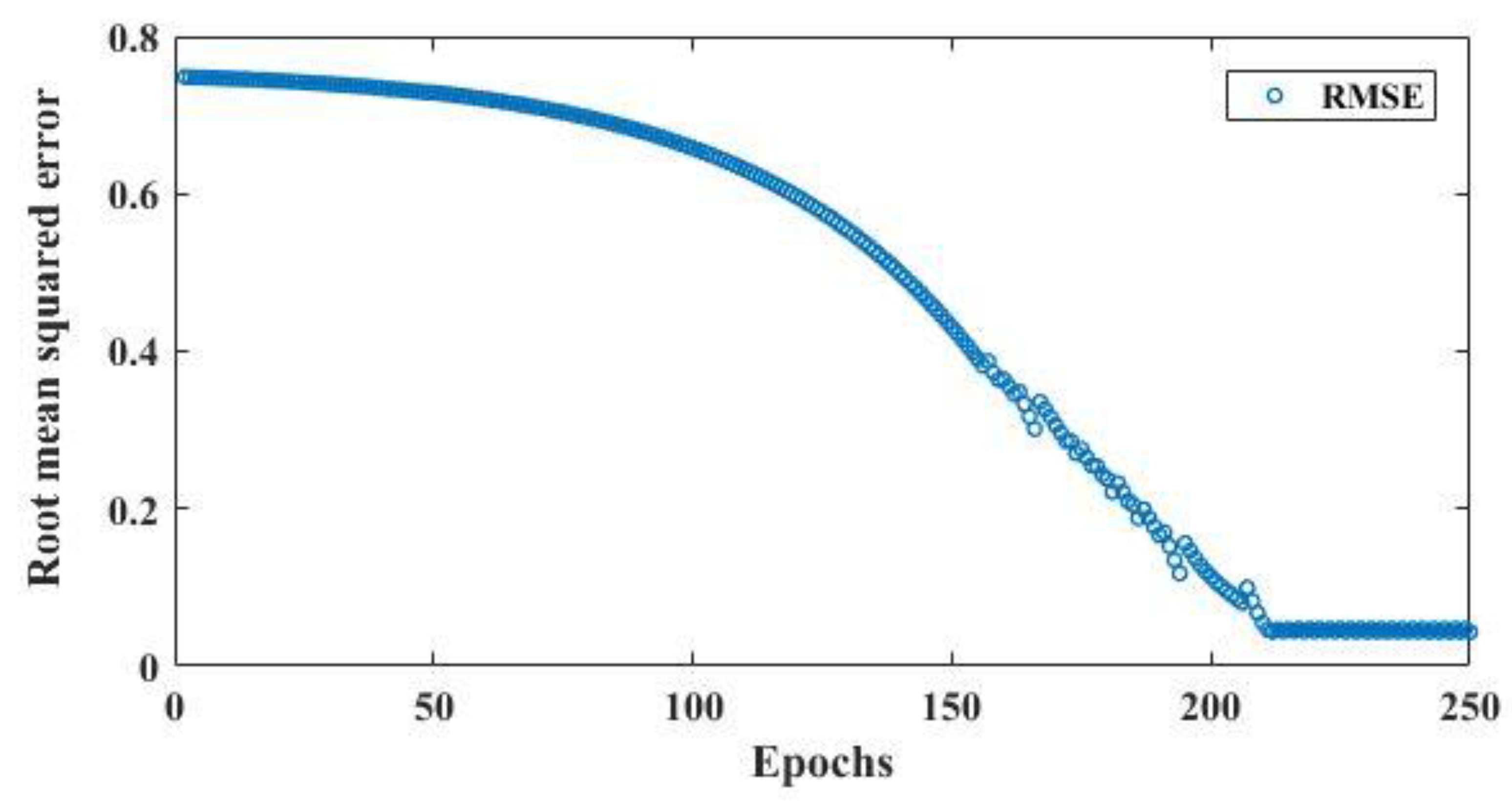
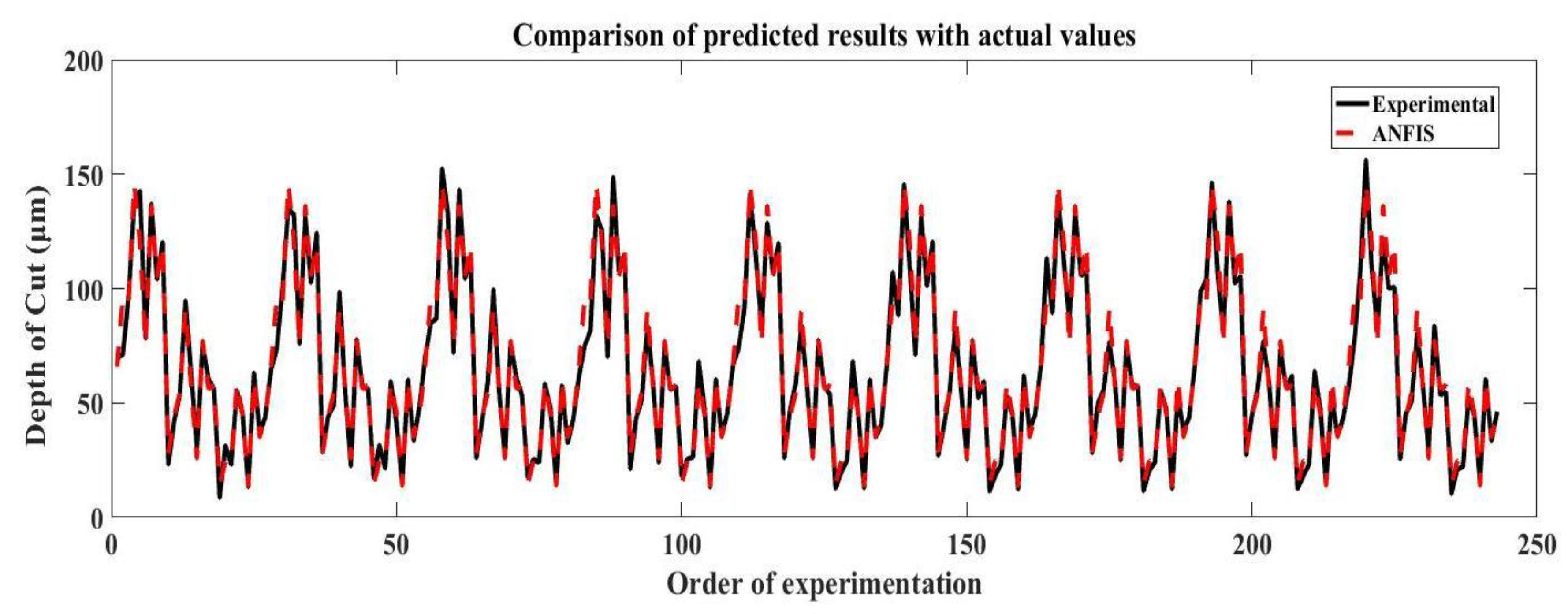
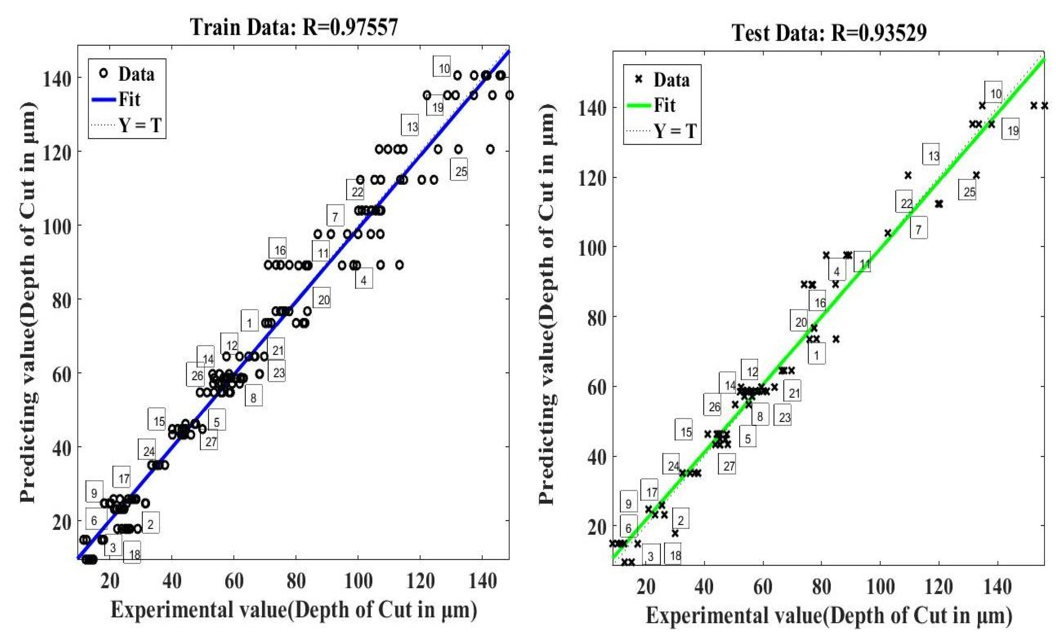
4.2.3. Training the Network and Prediction Performance

Prediction of the depth of cut of the process by ANFIS consists of two main parts; training data and testing data. Hence, among data sets, 70% data is selected stochastically for the training of the ANFIS network and 30% for testing the developed model.

During the training in ANFIS, 27 sets of data were used to conduct learning, and this ceased after 250 iterations, as shown in Figure 15. The step size for parameter adaptation had an initial value of 0.1. The proposed ANFIS training parameters are given in

Table 4. Adaptive Neuro-Fuzzy Inference System (ANFIS) training parameters.

Parameter	Value
Neuron level	5
Size of input data set	243
Training Set	70%
Testing Set	30%
andMethod	Prod
orMethod	Max
defuzzMethod	Wtaver
impMethod	Prod
aggMethod	Max
Number of output	1
Membership function	Sigmoidal membership
Learning rules	Least square estimation-Gradient descent algorithm
Number of epoch	250

. Adaptive neuro-fuzzy inference system (ANFIS) learning in this work uses the hybrid method for updating membership function parameters, which are comprised of back-propagation for the parameters linked with the input membership and least-squares estimation for the parameters related to the output membership functions. The results projected from the fuzzy model of belt grinding have been assessed with the experimental data for validation. Figure 16 gives the comparison of the predicted depth of cut using the established fuzzy model and the data taken from the belt grinding experiments.

The developed ANFIS system gave an overall 93.5% accuracy, as illustrated in Figure 17. Comparing outputs generated by the fuzzy model with the experimental data from 27 test conditions based on Taguchi DoE (Design of Experiments), the variations are found to be minimum. Thus, it can be inferred that there is a co-relation between the simulated results and the experimental results obtained at the same machining conditions.

5. Conclusions

In this study, an investigation into the influence of belt grinding parameters on material removal depth based on the Taguchi parameter design method has been analysed and presented. In the belt grinding experiments, three levels of cutting wheel speed, feed rate, force, grit size, and polymer hardness were applied. Based on the experimental results and summarising the research, the following generalised conclusions are drawn:

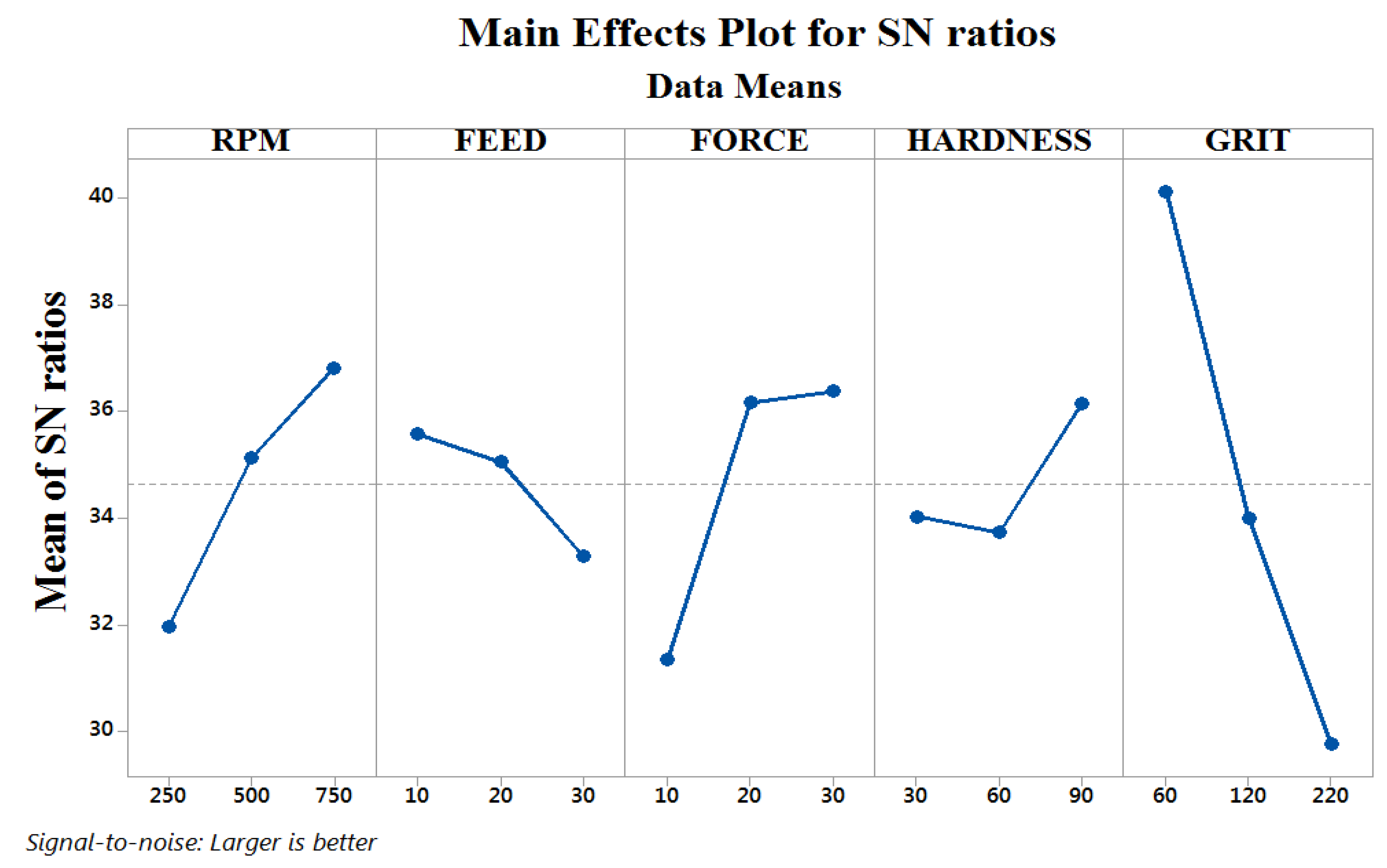
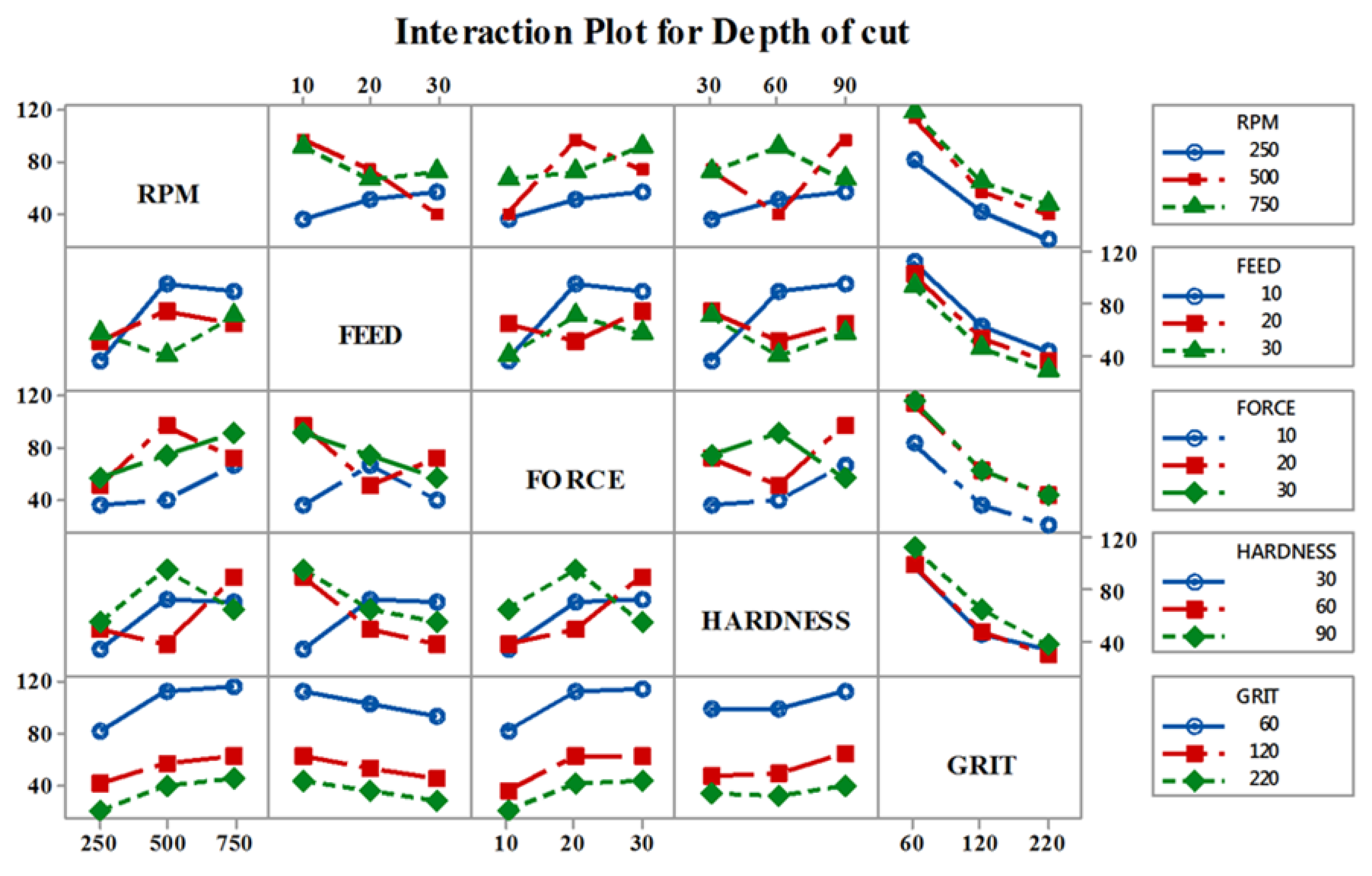
• ANOVA determined the level of significance of the machining parameters on the material depth of cut. Based on the analysis of variance (ANOVA) results at a 95% confidence level, the highly dominant parameters of material removal are identified. Namely, the grit size grinding parameter is the primary factor that has the highest influence on the material removal, and this parameter is about five times greater than the second ranking parameters (RPM and force imparted). The feed rate and polymer wheel hardness parameters do not seem to have much of an influence on the depth of cut, i.e., material removal. Results from ANOVA interactions also suggests that the experimental trials can further be optimised using Taguchi Interaction instead of orthogonal design.
• Based on the signal-to-noise ratio results in Figure 9, we can construe that 750 RPM, 10 mm/s feed rate, 30 N force, 90 Shore A hardness, and 60 grit size are the optimal grinding parameters for achieving maximum depth of cut.
• A method of modelling and calculating the material removal using ANFIS is proposed in this paper. The ANFIS model developed is validated with experimental trials for given conditions. It has been identified that results produced by the designed regression model have acceptable deviations between the predicted and the actual experimental results with 93.5% accuracy. The ANFIS model developed in this research work is viable and could be used to predict the depth of cut, i.e., material removal for an Abrasive Belt Grinding process.

References

1. Zhang, X.; Kuhlenkötter, B.; Kneupner, K. An efficient method for solving the Signorini problem in the simulation of free-form surfaces produced by belt grinding. Int. J. Mach. Tools Manuf. 2005, 45, 641–648. [Google Scholar] [CrossRef]
2. Jourani, A.; Dursapt, M.; Hamdi, H.; Rech, J.; Zahouani, H. Effect of the belt grinding on the surface texture: Modeling of the contact and abrasive wear. Wear 2005, 259, 1137–1143. [Google Scholar] [CrossRef]
3. Ren, X.; Cabaravdic, M.; Zhang, X.; Kuhlenkötter, B. A local process model for simulation of robotic belt grinding. Int. J. Mach. Tools Manuf. 2007, 47, 962–970. [Google Scholar] [CrossRef]
4. Ren, X.; Kuhlenkötter, B.; Müller, H. Simulation and verification of belt grinding with industrial robots. Int. J. Mach. Tools Manuf. 2006, 46, 708–716. [Google Scholar] [CrossRef]
5. Hamann, G. Modellierung des Abtragsverhaltens Elastischer Robotergefuehrter Schleifwerkzeuge; University of Stuttgart: Stuttgart, Germany, 1998. [Google Scholar]
6. Rufeng, X.; Chen, Z.; Chen, W.; Wu, X.; Zhu, J. Dual drive curve tool path planning method for 5-axis NC machining of sculptured surfaces. Chin. J. Aeronaut. 2010, 23, 486–494. [Google Scholar] [CrossRef]
7. Zhang, X.; Kneupner, K.; Kuhlenkötter, B. A new force distribution calculation model for high-quality production processes. Int. J. Adv. Manuf. Technol. 2006, 27, 726–732. [Google Scholar] [CrossRef]
8. Radzevich, S.P. A closed-form solution to the problem of optimal tool-path generation for sculptured surface machining on multi-axis NC machine. Math. Comput. Model. 2006, 43, 222–243. [Google Scholar] [CrossRef]
9. Pi, J.; Red, E.; Jensen, G. Grind-free tool path generation for five-axis surface machining. Comput. Integr. Manuf. Syst. 1998, 11, 337–350. [Google Scholar] [CrossRef]
10. Taguchi, G. Introduction to Quality Engineering: Designing Quality into Products and Processes; Asian Producativity Organization: Tokyo, Japan, 1986. [Google Scholar]
11. Lindman, H.R. Analysis of Variance in Experimental Design; Springer Science & Business Media: New York, NY, USA, 2012. [Google Scholar]
12. Gill, S.S.; Singh, J. An Adaptive Neuro-Fuzzy Inference System modeling for material removal rate in stationary ultrasonic drilling of sillimanite ceramic. Expert Syst. Appl. 2010, 37, 5590–5598. [Google Scholar] [CrossRef]
13. Çaydaş, U.; Hasçalık, A.; Ekici, S. An adaptive neuro-fuzzy inference system (ANFIS) model for wire-EDM. Expert Syst. Appl. 2009, 36, 6135–6139. [Google Scholar] [CrossRef]
14. Jang, J.-S.R. ANFIS: Adaptive-network-based fuzzy inference system. IEEE Trans. Syst. Man Cybern. 1993, 23, 665–685. [Google Scholar] [CrossRef]
15. Wang, S.; Li, C. Application and development of high-efficiency abrasive process. Int. J. Adv. Manuf. Technol. 2012, 47, 51–64. [Google Scholar]
16. Huang, H.; Gong, Z.M.; Chen, X.Q.; Zhou, L. Robotic grinding and polishing for turbine-vane overhaul. J. Mater. Process. Technol. 2002, 127, 140–145. [Google Scholar] [CrossRef]
17. Lei, Y.; He, Z.; Zi, Y. A new approach to intelligent fault diagnosis of rotating machinery. Expert Syst. Appl. 2008, 35, 1593–1600. [Google Scholar] [CrossRef]
18. Ying, L.-C.; Pan, M.-C. Using adaptive network based fuzzy inference system to forecast regional electricity loads. Energy Convers. Manag. 2008, 49, 205–211. [Google Scholar] [CrossRef]
19. Zadeh, L.A. Fuzzy sets. Inf. Control 1965, 8, 338–353. [Google Scholar] [CrossRef]
20. Werbos, P.J. Backpropagation through time: What it does and how to do it. Proc. IEEE 1990, 78, 1550–1560. [Google Scholar] [CrossRef]
21. Yilmaz, O.; Bozdana, A.T.; Okka, M.A. An intelligent and automated system for electrical discharge drilling of aerospace alloys: Inconel 718 and Ti-6Al-4V. Int. J. Adv. Manuf. Technol. 2014, 74, 1323–1336. [Google Scholar] [CrossRef]
Figure 1. Principle of belt grinding process.
Applsci 07 00363 g001
Figure 2. Adaptive neuro-fuzzy inference system structure.
Applsci 07 00363 g002
Figure 3. Belt Sander customised to perform grinding experimental trials.
Applsci 07 00363 g003
Figure 4. Experimental setup for compliant Abrasive Belt Grinding.
Applsci 07 00363 g004
Figure 5. Toolpath planning in force control mode by ABB Robot Studio.
Applsci 07 00363 g005
Figure 6. Profilometer with the tactile stylus used to measure the depth of cut across the grinded path at three different locations A, B and C.
Applsci 07 00363 g006
Figure 7. (a) 3D profile extracted from the workpiece surface across the machined surface using Taly-scan; (b) 2D profile obtained from the workpiece surface across the grinded path to measure the depth of cut.
Applsci 07 00363 g007
Figure 8. Standard deviation of the depth of cut taken from Taguchi based L27 orthogonal experimental trials.
Applsci 07 00363 g008
Figure 9. Mean signal-to-noise (S/N) ratio graph for depth of cut.
Applsci 07 00363 g009
Figure 10. Two way interaction effect plots between RPM, feed, force, hardness, and grit and their influence on depth of cut at different initial levels of parameters.
Applsci 07 00363 g010
Figure 11. Adaptive Neuro-Fuzzy Inference System (ANFIS) model for belt grinding showing inputs and output.
Applsci 07 00363 g011
Figure 12. Topology of adaptive neuro-fuzzy inference system architecture.
Applsci 07 00363 g012
Figure 13. A part of the rule viewer in the proposed fuzzy model.
Applsci 07 00363 g013
Figure 14. Change in shape of the sigmoidal membership function for each input before and after Training.
Applsci 07 00363 g014
Figure 15. Plot of error versus epochs for modelling material removal.
Applsci 07 00363 g015
Figure 16. Comparison of predicted with actual experimental values for depth of cut.
Applsci 07 00363 g016
Figure 17. Correlation between actual and predicted values of test and train data set.
Applsci 07 00363 g017