
Development of Height Indicators using Omnidirectional Images and Global Appearance Descriptors


Miguel Hernandez University, Department of Systems Engineering and Automation, Avda. de la Universidad s/n. Ed. Innova. 03202, Elche (Alicante), Spain
*
Author to whom correspondence should be addressed.
†
These authors contributed equally to this work.
Appl. Sci. 2017, 7(5), 482; https://doi.org/10.3390/app7050482
Submission received: 9 March 2017
/
Revised: 2 May 2017
/
Accepted: 4 May 2017
/
Published: 6 May 2017
Abstract
:Nowadays, mobile robots have become a useful tool that permits solving a wide range of applications. Their importance lies in their ability to move autonomously through unknown environments and to adapt to changing conditions. To this end, the robot must be able to build a model of the environment and to estimate its position using the information captured by the different sensors it may be equipped with. Omnidirectional vision sensors have become a robust option thanks to the richness of the data they capture. These data must be analysed to extract relevant information that permits estimating the position of the robot taking into account the number of degrees of freedom it has. In this work, several methods to estimate the relative height of a mobile robot are proposed and evaluated. The framework we present is based on the global appearance of the scenes, which has emerged as an efficient and robust alternative comparing to methods based on local features. All the algorithms have been tested with some sets of images captured under real working conditions in several indoor and outdoor spaces. The results prove that global appearance descriptors provide a feasible alternative to estimate topologically the relative altitude of the robot.
1. Introduction
Over the last few years, mobile robotics has become a technology that has gained presence in many kinds of environments to solve different problems, both in industries, educative centres and in households. To increase their range of applications, mobile robots must be able to solve the task they have been designed for in a truly autonomous way. With this aim, two crucial abilities must be developed: the robot must be able to build a model of the environment where it has to move and to estimate its position and orientation within this model.
Mobile robots may be equipped with different kinds of sensors that provide them with information that permits solving the mapping and localization problems. These sensors can be categorised into proprioceptive and exteroceptive. On the one hand, proprioceptive sensors measure the state of the robot. Encoders installed in the wheels are an example. Through an odometry process they permit estimating the displacement of the robot, but the error in this estimation tends to grow indefinitely. This is why enconders tend to be used in combination with other sources of information [1]. On the other hand, exteroceptive sensors measure some information from the environment where the robot is moving. Among them, some researchers have made use of GPS, SONAR and laser sensors in previous works. First, GPS (Global Positioning Systems) constitute a robust choice outdoors, but the information they provide close to buildings and on narrow streets is less reliable [2]. Second, SONAR and laser sensors permit measuring the distance to the objects around the robot using different technologies. The use of laser sensors has extended substantially in mobile robotics [3] because they tend to present an improved precision and angular resolution comparing to SONAR. Nevertheless, they also present a higher cost, weight and power consumption.
More recently, vision sensors have gained popularity because they present several advantages. They capture a big quantity of information from the environment, which can be used to carry out many high level tasks, apart from mapping and localization, such as people and objects detection and recognition. They also present a relatively low cost and power consumption comparing to laser rangefinders and the information they provide is stable both outdoors and indoors, unlike GPS, whose signal tends to degrade indoors. Vision sensors can be used either as the only source of information from the environment or in combination with other kinds of sensors [4]. Initially, monocular configurations were used but later works tried to expand the field of view through other configurations such as binocular [5] or omnidirectional [6,7,8]. In recent years, the use of omnidirectional vision sensors has expanded thanks to the big quantity of information they capture (as they are able to take images with a field of view of 360 deg around the robot) with a relatively low cost. Nevertheless, working with omnidirectional visual data is a complex task when the robot has to create models of large and complex environments while moving with more than 3 Degrees Of Freedom (DOF). In these cases, it is necessary to extract some information from the scenes to build a robust model that gathers relevant and invariant knowledge from the environment and that permits estimating the position of the robot with the required DOF. Extracting this useful information from the scenes is a key point since images are very high dimensional data that change not only when the robot moves along any DOF but also under other circumstances such as variations in lighting conditions.
Two main approaches have been used by the researchers to compile such information. On the one hand, some relevant landmarks or outstanding points or regions (either natural or artificial) can be extracted and described using any local descriptor that captures the appearance of the landmarks’ neighbourhood trying to get invariance to position, scale and rotation [9,10,11,12]. On the other hand, each scene can be represented through a unique global appearance descriptor that contains information on the whole scene [13,14,15,16].
Many authors have addressed the mapping and localization problems using vision sensors. The different approaches proposed can be roughly classified into three different types, depending on the contents and the internal structure of the models. First, a metric map can be built trying to define the position of some outstanding points of the environment with respect to a reference system. These models permit estimating the position of the robot with geometrical accuracy up to a specific error [17,18,19]. Second, topological maps usually represent some characteristic places of the environment and the connectivity relationships between them. They tend to be simpler representations but they contain usually enough details for most applications [20]. Third, hybrid maps try to gather the advantages of the two previous approaches. They arrange the information into several layers with different levels of detail, containing topological models in the top layers that permit a rough localization and metric models in the bottom layers to refine this localization [21,22,23].
Traditionally, metric maps have been built using methods based on the extraction, description and tracking of local features along a set of scenes captured by the vision sensor mounted on the robot. This information is often combined with other sources of information, such as odometry or laser [24]. However, these models tend to be quite complex and not easily interpretable by a human operator, and the localization process is usually elaborated and computationally expensive. In contrast, topological maps offer more intuitive representations of the environment [25]. Visual global-appearance approaches may be used to create such models, since no metric information can be extracted from global descriptors. They lead to simpler models where the localization process is more straightforward, based mainly on the pairwise comparison between image descriptors [26].
The problem of robot localization using visual models of the environment has been thoroughly studied when the trajectory of the robot is contained in the ground plane. Researchers have made use both of local features [27] and global appearance [28] to build image descriptors that permit solving this problem. Beyond that, in some applications, it may be useful to estimate the altitude of the robot with respect to this plane, without changing the visual map nor including any further visual information. The proposal of the present work fits within this area. The main objective consists in extracting some information from the images that permits estimating the relative altitude of the robot, using the previously built visual model of the environment.
About the choice of the approach to describe the scenes, some researchers have addressed the altitude estimation problem using local descriptors [29,30,31,32]. However, the literature on altitude estimation using only visual information and global appearance descriptors is quite sparse and few works can be found on this topic, despite the advantages that global appearance descriptors can offer to the mapping and localization problems [33]. Taking this into account, this work is focused on studying the performance of global-appearance methods to solve this problem. The only source of information used is a catadioptric vision sensor mounted on the mobile platform.
The contribution of this paper is twofold. On the one hand, some global appearance approaches are defined to incorporate the altitude information in the descriptors and some methods are proposed to estimate robustly this relative altitude without changing nor including any additional information to the visual model of the environment. On the other hand, a comparative evaluation of these methods is carried out to analyse their behaviour both indoors and outdoors. The altitude estimators we propose go beyond the classical topological notion of connectivity and introduce the concepts of closeness and farness, thus some altitude estimators are proposed that estimate the relative height of a robot except for a scale factor. The results of this paper jointly with the developments presented in [26,34] prove the usefulness of the global appearance descriptors to estimate the position and orientation of the robot in the ground plane and its altitude with respect to this plane, in a straightforward way. This supposes a step ahead towards the definition of global appearance descriptors that permit building models of the environment and localization when the robot moves with 6 DOF.
The remainder of the paper is structured as follows. Section 2 makes a review of some techniques to describe globally the appearance of omnidirectional visual information. Then, in Section 3 the methods implemented to estimate topological height from visual information are detailed. After that, Section 4 describes the geometry of the vision system and the sets of images used to carry out the experiments, whose results are presented in Section 5. At last, the conclusions and future works are outlined in Section 6.
2. Omnidirectional Imaging and Global Appearance Descriptors
Along the paper, the use of omnidirectional visual information along with global appearance descriptors is proposed to develop some height indicators. This section presents some fundamentals on the kind on sensors used to obtain the omnidirectional images (Section 2.1) and on the mathematical methods used to describe the global appearance of these images (Section 2.2). The information contained in these descriptors will be used in Section 3 to estimate topological height.
2.1. Catadioptric Vision Sensors
Catadioptric vision sensors consist of a conventional camera pointing towards a convex mirror with their axes aligned. In this work, a hyperbolic mirror will be considered and the axes of the mirror and the camera will be always parallel to the z-axis of the world reference system. The world information reflects onto the mirror and the camera captures this reflection, composing the omnidirectional image. Figure 1 shows the projection model of the catadioptric vision system, showing the World Reference System (WRS), the Camera Reference System (CRS), centered on the focal point of the hyperbolic mirror , and the Image Reference System (IRS). F is the focal point of the camera. The figure shows the projection of a world point P onto the mirror Q and from the mirror to the image plane m. The image projected onto the image plane (plane of projection) is the omnidirectional view. The calibration of the catadioptric system provides us with a function that permits calculating, for each pixel in the image, the coordinates of the point of the mirror that has produced this pixel, respect the CRS [35]. a is the distance between the pixel considered and the center of the image, expressed in pixels. From the omnidirectional image, other projected versions of the visual information can be obtained, such as the cylindric projection (panoramic image), the orthographic projection (projection onto a plane) or the unit sphere projection [36]. Figure 2 shows (a) a sample omnidirectional image and three different projections obtained from it; (b) orthographic projection onto a plane parallel to the ground plane; (c) unit sphere projection and (d) cylindrical projection or panoramic view.
2.2. Global Appearance Descriptors
Descriptors based on the global appearance of images captured by a catadioptric vision system have proved a good performance both in position and orientation estimation, when the movement of the robot is restricted to the floor plane, as Gaspar et al. [36] and Payá et al. [26] show. These methods extract the most relevant information from each image and reduce the amount of memory necessary to store the visual information working with the image as a whole, i.e., avoiding the extraction of landmarks or local features. In this work, three different techniques based on the Discrete Fourier Transform (DFT) are considered: the Fourier Signature (FS), the two-dimensional Discrete Fourier Transform (2D-DFT) and the Spherical Fourier Transform (SFT). In the next subsections a brief outline of these description methods is made and some relevant mathematical properties are presented. After that, in Section 3 some methods are proposed to develop height indicators using these description methods and their properties.
2.2.1. Fourier Signature
The Fourier Signature (FS) was firstly described by Menegatti et al. [37], who used it to carry out mapping and localization with a robot whose movement is restricted to the ground plane. It consists in the representation of a panoramic image calculating the one-dimensional DFT of each row. Therefore, each row of the original image , can be transformed into the sequence of complex numbers .
When the DFT of every row of the image is calculated, a new matrix is obtained, being u the frequency variable (cycles/pixel). The components of this matrix are complex numbers thus it can be decomposed into a magnitudes matrix and an arguments matrix . Taking the properties of the DFT into account [37], only a subset of k columns can be retained to represent the image: and , .
The FS presents another interesting property when used to describe a panoramic image. If the image comes from an omnidirectional vision sensor mounted vertically on the robot, then, the modules matrix is invariant against rotations around the vertical axis. Let’s consider two panoramic images captured from the same position on the ground plane but having the robot different orientations with respect to the vertical axis, with relative orientation , as shown in Figure 3. If the row m of the first image is represented as the sequence , then the same row in the second (rotated) image is , where q is the shift between images, measured in pixels, which is proportional to the relative rotation between images , where is measured in deg. Visually this shift appears as a circular shift of the columns of the image (Figure 3).
The rotational invariance can be expressed by the DFT shift theorem as:
where is the one-dimensional DFT of the shifted sequence, and are the components of the one-dimensional DFT of the non-shifted sequence (row ).
Taking this theorem into account, when the movement of the robot is contained in the ground plane, the magnitudes matrix can be used to estimate the position (since it is invariant to rotation), and the arguments matrix to estimate the relative orientation.
2.2.2. Two-dimensional Discrete Fourier Transform
The two-dimensional Discrete Fourier Transform (2D-DFT) of an image can be expressed as a new matrix that can be split into two matrices, one containing the magnitudes (or power spectrum) and other with the arguments . Since the most relevant information in the Fourier domain concentrates in the low frequency components and the high frequency information is usually more affected by noise, retaining only a number of low frequency components may lead to better results in localization with an improved computational cost. Taking this fact into account, the number of rows retained from the matrices A and will be and the number of columns .
Another interesting property when working with panoramic images is the rotational invariance, which is reflected in the shift theorem:
where is the 2D-DFT of the original image and is a shifted version of this image. According to this theorem, the power spectrum of the shifted image remains the same of the original image and only a change in the argument of the components of the transformed image is produced, whose value depends on the shift along the -axis () and the -axis (). Thanks to this property, this transform has previously been used to estimate the position and orientation of a robot when it moves on the ground plane [26]. In this case, if the robot captures two panoramic scenes and from the same position on the ground plane but with different orientations, the magnitudes matrices and are the same and only a shift along the -axis is produced, which can be calculated from the theorem and used to estimate the relative orientation.
Equation (2) also shows that the first row of the 2D-DFT, which corresponds with , is only affected by shifts along the -axis of the image, whereas the first column of the transform, which corresponds with , is only affected by shifts along the -axis.
2.2.3. Spherical Fourier Transform
Omnidirectional images can be projected onto the unit sphere when the intrinsic parameters of the catadioptric vision system are known. Being the colatitude angle, and the azimuth angle, the projection of the omnidirectional image onto the 2D sphere can be expressed as . As shown in [38], the spherical harmonic functions form a complete orthonormal basis over the unit sphere. Any square integrable function defined on the sphere can be represented by its spherical harmonic expansion as:
with and , . denotes the spherical harmonic coefficients, and the spherical harmonic function of degree l and order m defined by:
where are the associated Legendre functions.
It is also possible to build a rotationally invariant representation of omnidirectional images using the Spherical Fourier Transform (SFT). Considering B the band limit of f, the coefficients of are not affected by 3D rotations of the signal, where:
More information and examples of applications of the SFT in navigation tasks can be found in [39,40,41,42]. Makadia et al. [39] introduce the estimation of 3D rotations extending the shift theorem to the SFT. Schairer et al. [40] present a rotation estimation algorithm based on the SOFT (SO(3) Fourier Transform), being SO(3) the 3D Rotation Group. On the other hand, Huhle et al. [41] and Schairer et al. [42] show a localization method using the SFT applied to omnidirectional images and a predictive model of Gaussian probabilistic regression.
In this work, we take advantage of the rotational invariance properties of the DFT to describe the scenes, using with this aim.
3. Development of Height Indicators Using Global Appearance Descriptors
Our previous works [26,34] have focused on building a visual model of the environment and estimating the position of the mobile platform when its movement is contained in the ground plane, using the global appearance of the scenes with this aim. However, as stated previously, it is also interesting to study the possibility of estimating the altitude of the vehicle with respect to the plane where it moved when the visual model was created. With this goal, several methods are proposed in this section and analysed in the subsequent sections in order to know the accuracy and advantages of each one.
In all cases, only visual information will be used to estimate the relative altitude. The two images to compare are named reference and test image ( and respectively) and the algorithms estimate the height of with respect to . Since the objective of this work consists in studying the performance of some methods in altitude estimation, we consider the images to compare have been captured along a line which is parallel to the z-axis of the WRS, being the axis of the catadioptric system in vertical position (Figure 1). This way, we isolate the effect of height changes in the images.
To compare two scenes using their global appearance, a distance measurement must be defined. In this work, the image distance is defined as the Euclidean distance between descriptors. Being the descriptor of the test image, and the descriptor of the reference image, the image distance can be obtained as:
The best match among a set of different comparisons is found by choosing the one with minimum distance.
The next subsections present the relative height estimation methods in detail. Four methods based on global appearance have been implemented and tested. They are based on the descriptors presented in Section 2.2. Also, for comparative purposes, an additional method that uses local features is proposed in Section 3.5.
3.1. Method 1: Central Cell Correlation of Panoramic Images
In a panoramic image, the most distinctive information is usually in the central rows of the scene. In outdoor environments, the bottom rows normally correspond to the terrain, and the upper rows to the sky and in indoor environments they correspond to the floor and ceiling respectively. If the altitude of the catadioptric system changes whether upwards of downwards, the area constituted by the central rows of the panoramic image is less likely to go out of the camera field of view. Taking this fact into account, in this method, the global appearance of the central rows of the reference and test images is compared to estimate the relative height between their capture points.
First, the algorithm computes a global appearance descriptor of the central cell of (the portion composed by the central rows). To obtain this descriptor either the FS (Section 2.2.1) or the 2D-DFT (Section 2.2.2) can be used. This process is repeated for different cells situated above and below the central cell. In Figure 4 a sample image and some cells extracted from it are shown. The central cell is emphasized with a wider line, and some additional cells have been defined both above and below it. d is the vertical distance (measured in pixels) from each additional cell to the central one.
Considering now a test image , the algorithm computes the descriptor of the central cell, compares it with all the descriptors of the cells extracted from and retains the best match. The position (d) of the cell in that best matches the central cell of is a measurement of the relative altitude. Therefore, the displacement is measured in pixels and it can be considered as a topological distance
To illustrate this method, two panoramic images captured from different heights are considered (Figure 5). On the one hand, Figure 5a is the reference image (). On the other hand, Figure 5b is the test image () and it was captured from a height 60 cm higher than . In this example, the size of the cells is equal to pixels and FS is used to describe these cells.
First, is considered and its central cell is extracted. After that, the FS of this cell is calculated and its magnitudes matrix is obtained. The result is the descriptor , where the superscript indicates that this is the descriptor of the central cell. This process is repeated for different cells situated above and below the central cell. To do it, a set of cells is considered, whose distances to the central cell are, in this example, pixels. After that, the descriptors of the cells will be available, where the superscript indicates the distance to the central cell.
Second, is considered. Its central cell is extracted, the FS of this cell is calculated and the magnitudes matrix is obtained. The result is the descriptor .
When all this information is available, the algorithm calculates the Euclidean distance (Equation (6)) between the descriptor and each of the descriptors , considering . The distance d associated to the descriptor that best matches can be considered as a height indicator. Figure 6 shows versus d. In this case, the minimum is produced at . Since , the height of is higher than .
3.2. Method 2: 2D-DFT Vertical Phase
This method is based on the use of the 2D-DFT and the shift theorem presented in Section 2.2.2. Traditionally, this method has been used to estimate the relative orientation of the robot with respect to the vertical axis when its movement is contained in the ground plane [26]. In this case, a change in the orientation of the robot produces a circular shift of the columns of the panoramic image which can be estimated through the shift theorem (Equation (2)).
Besides, this descriptor can also be used to estimate relative height since a vertical displacement of the robot will produce a shift of the rows of the panoramic image that can also be estimated through the shift theorem. However, the use of the theorem in this case is not direct because, unlike a rotation around the vertical axis, a vertical movement does not produce a circular shift of rows and the information in the scene is thus modified; after the vertical displacement some rows of the original image will go out and new rows will appear. Taking this fact into account, the magnitudes matrix of the transformed image will experience some changes hence the shift theorem is not exactly met.
Despite the issues described above, the preliminary experiments showed that the great majority of the visual information remains after a vertical displacement therefore a circular shift of the image’s rows will be assumed when using this method. For this reason, in order to estimate topologically the vertical displacement between the reference and the test images, we use the arguments matrices of their 2D-DFT, and , where only the first components have been retained. We consider .
As stated before, a vertical movement in the spatial domain produces a change in the phase of the coefficients in the frequency domain. Our approach simulates different shifts on the matrix (using Equation (2)), compares each shifted matrix with and retains the shift that produces the best match. A circular shift of S deg of the rows of the reference image produces a change on its arguments matrix that can be simulated through the next expression:
where is the Vertical Rotation Matrix, defined as:
To illustrate this property we consider a sample panoramic image , where and . From it, a new image with the same size is generated, considering a circular shift of rows (the displacement is towards the top of the image). This is equivalent to generating a shift deg. The original and the shifted images are shown in Figure 7a,b respectively.
Using these two images, the next sequence of operations is carried out. First, the 2D-DFT of both images is calculated, resulting the matrices and . Second, the magnitudes and the arguments matrices of both transforms are obtained and just the first rows and columns are retained. Equation (9) shows the two magnitudes matrices and Equation (10) the two arguments matrices, expressed in the range deg.
On the one hand, Equation (9) shows that both magnitudes matrices are identical, as expected according to Equation (2). On the other hand, the relationship between both arguments matrices meets Equation (7), as detailed in the next equation:
Taking all these facts into consideration the next steps are followed in the height estimation application. First, from the reference image , a set of rotated versions is generated considering . In the experiments, is given a value equal to .
Second, when a new test image arrives, the arguments matrix of its 2D-DFT is obtained and compared with the set of matrices generated from the reference image. The coefficient S that produces the best match (the minimum distance) is a topological measurement of the relative altitude between images.
3.3. Method 3: Multiscale Analysis of the Orthographic View
In this method a multiscale analysis is carried out to estimate the relative height. This analysis consists in carrying out several artificial zoomings of the central area of the scenes and has been used previosly to estimate the topological distance between the capture points of two scenes when the robot moves in the ground plane [43]. To obtain consistent results, the projection plane of the images must be perpendicular to the direction of the movement. Since we consider vertical movements in this work, an orthographic projection of the omnidirectional image onto a horizontal plane must be used.
The method consists in generating several orthographic projections of the reference image, considering different focal distances to the plane where the image is projected. This is equivalent to generating a set of orthographic projections with different zooms. Figure 8 shows a sample omnidirectional image and three of its orthographic views, assuming three different focal distances for the projection plane.
After that, the different projections are described using global appearance. This way, a set of descriptors is generated from , each one with a focal distance associated: .
When a new omnidirectional test image arrives, the algorithm computes an orthographic view with a specific focal distance and calculates its descriptor, obtaining the pair . Next, the descriptor of the test image is compared with all the descriptors of the reference image and the best match (minimum distance) is retained.
We retain the focal distance of the reference image where the minimum is found, . The difference between the focal distance of the test image projection and the focal distance of the matched reference image projection is a topological measurement of relative height: .
In the experiments, the set of focal distances for the reference image are generated in the range = [4, 11], while the focal distance of the test image is .
3.4. Method 4: Change of the Camera Reference System (CRS)
The fourth method consists in simulating an artificial movement of the camera and calculating the new coordinates of the pixels of the image after the movement. Some researchers (such as Valiente et al. [44]) have used this technique to simulate a displacement of the Camera Reference System (CRS) using the epipolar geometry.
To obtain the new image after the artificial displacement, the next steps are followed. First, each pixel of the original omnidirectional image is retroprojected to obtain its coordinates with respect to the WRS. Let be the coordinates of one pixel of the omnidirectional image (with respect to the IRS) and a the distance from this pixel to the center of the omnidirectional image. The function (an example is shown in Equation (15)), obtained from the calibration of the catadioptric system, permits calculating the point of the mirror Q that projects onto this pixel m. This point can be retroprojected onto the unit sphere and, as a result, the coordinates of this projection respect to the CRS can be obtained. After that, a movement of the camera is simulated through a change of the CRS and the new coordinates respect the new CRS system will be:
being the unitary displacement vector, and the scale factor, which is proportional to the amount of displacement. In this work, to simulate a vertical displacement .
Using the new coordinates of the projection of the point onto the unit sphere , the corresponding point on the mirror can be obtained and projected onto the new image plane, where the new coordinates respect the IRS will be . Repeating this operation for all the pixels of the original image, the result will be the new omnidirectional image after the simulated movement. After this process, some pixels of the original image may lay out the new image plane and some pixels of the new image may be empty. In this case, the value of these pixels is estimated as the average value of its 8 nearest neighbours.
Once the new omnidirectional image after the artificial movement has been calculated, different projections can be obtained. Specifically, in this work, the orthographic view, the panoramic image and the unit sphere projection are considered. Figure 9 shows the simulated vertical movement of the catadioptric system. On the one hand, Figure 9a shows the projection of a world point P onto the original image plane m (plane of projection 1) and onto the new image plane after the simulated vertical movement (plane of projection 2) obtained using epipolar geometry. and are the focal points of the hyperbolic mirror before and after the movement and and are the focal points of the camera. On the other hand, Figure 9b shows two sample omnidirectional images and panoramic projections considering the original image plane () and the new image plane after the simulated movement ().
In order to estimate the relative height between two scenes, the algorithm simulates several displacements of the reference image by giving different values to , and compares each of them with the test image , considering , i.e., without CRS movement, and using global appearance. Finally, the algorithm selects the best match. The coefficient associated with this match is a topological measurement of the vertical distance between images. In the experiments, the coefficient of the reference image will be given values between and .
3.5. Method 5: Matching of SURF Features
The last method makes use of local features extracted from the omnidirectional scenes to estimate topological height. SURF features are used with this aim [45]. This method has been introduced for comparative purposes, since using local features is a mature approach to solve the localisation problem.
The method starts extracting and describing the SURF features of the reference and test omnidirectional scenes. After that, a matching process is carried out; the points of the test image are matched with the points of the reference image. Considering a purely vertical movement, the points of the test image will move along the radial direction, towards the centre of the image if the movement is upwards and towards the periphery if the movement is downwards.
Taking this fact into account, the matching process can be optimized by searching the possible match along the radial line associated to each point in the test image. Figure 10a shows two sample omnidirectional images captured indoors and superimposed, with a relative vertical movement between them. The SURF points have been extracted from the reference image (red points) and from the test one (green crosses), described, and matched (yellow lines show the matches). This figure shows a number of outliers (those matches which are not produced in the radial direction). Figure 10b shows the same two images, but the matches of the test image SURF points have been searched along the radial line in the reference image. In these sample images, the local features of the test image tend to be closer to the centre of the image. This means that the robot has moved upwards to capture the test image with respect to the reference one.
If and are, respectively, the set of SURF points extracted and matched from the reference and the test image (where the point matches the point ), then, the average distance between each pair of matched points (Figure 10b) can be considered as a topological measurement of the height difference between images:
where is the Euclidean distance between and . This distance is considered positive when is closer to the centre than and negative otherwise. This indicator is expected to provide a topological estimation of height. Furthermore, its linearity will depend on how linear the average displacement of the corresponding SURF points is when the omnidirectional vision system changes its altitude.
A popular alternative to obtain more robust results from the corresponding landmarks is the use of RANSAC (RANdom SAmple Consensus) [46]. An example of application in mobile robotics can be found in [47]. This way, in this paper, we also propose using RANSAC to estimate the relative topological altitude. Initially, a random subset of matched points can be used to have an estimation of the relative altitude, , calculated using Equation (14). After that, the rest of matched points can be used to corroborate this estimation. A pair of matched points corroborates this estimation if the distance between them is equal to plus or less a specific threshold. After repeating this process a number of times with different initial subsets of matched points, the estimation which is corroborated by a higher number of matched points is considered a measurement of the relative altitude.
During the experiments, both methods will be considered. First, the average distance between all the matched points will be calculated (the estimated height is ) and second, the RANSAC-based method will be considered () and the linearity of both methods will be assessed using a variety of images captured both indoors and outdoors.
4. Sets of Images
Several complete sets of images captured both indoors and outdoors have been used to test the five methods proposed in the previous section. They have been captured by ourselves inside and in the surroundings of the Innova building at Miguel Hernandez University (Spain), and they are available from [48]. In this section, the main features of these sets of images are presented.
The catadioptric vision sensor used consists of an Imaging Source DFK 21BF04 color camera with pixels resolution, and a hyperbolic mirror, whose model is Eizoh wide 70. Table 1 shows the main specifications of the mirror. Additional information on the mirror can be found in [49].
The camera has been adapted to a tripod that permits capturing images with a range of 165 cm along the z-axis of the WRS. Also, the mirror has been mounted above the camera, with their axes aligned. The distance between the focal points of the mirror and the camera is equal to 65 mm. Figure 11 shows the equipment used. The calibration of the camera has provided the following equation:
As stated in Section 2, this function permits obtaining the coordinates of the retroprojection of each pixel of the image onto the hyperbolic mirror with respect to the CRS. a represents the distance in pixels between the pixel considered and the center of the omnidirectional image.
To capture the sets of images, 21 positions have been defined on the ground plane indoors and outdoors. On each position a line parallel to the z-axis of the WRS has been considered and a set of images has been captured along each vertical line. Outdoors, 10 positions have been defined and 12 omnidirectional images per position have been captured, changing only the coordinate along the z-axis. This coordinate takes values between 125 cm and 290 cm with a gap of 15 cm between consecutive capture points. Indoors, 11 positions have been defined. The ceiling has limited the number of images captured from some positions. Table 2 shows the z-coordinate of each capture point and the number of images captured from each z-coordinate, considering both the oudoor and the indoor database. Figure 12 shows the position of the different ground positions above which each set of images has been captured. For each omnidirectional image, a cylindrical and an orthographic projection have been calculated with and pixels each.
About the choice of the capture positions, on the one hand, the outdoor images were captured both close to and far from buildings, in a parking area and gardens. Some sample omnidirectional images captured outdoors, from different positions, are shown in Figure 13. On the other hand, indoor scenes have been captured in several rooms of the building, including a laboratory, the hall and common areas. These rooms present very different visual appearances. Figure 14 presents 3 scenes of different indoor locations. The images have been captured in different times of the day in order to include different lighting conditions. Also, although the coordinates of each set and the orientation of the system around the z-axis are considered to be constant, the nature of the acquisition system has introduced small position and orientation changes between capture points. There are two main phenomena that produce these changes. On the one hand, the camera may suffer a small swing angle, due to the bending of the tripod. On the other hand, when changing the height of the tripod, the camera may experience a small change of orientation around the z-axis. In our experiments, the maximum value of both angles is equal to 3 deg. This way, it constitutes a challenging database that permits testing the algorithms under real working conditions. The whole set of images and more information on it is available on [48].
To see the effect that a height change has on the images, Figure 15 shows three images captured above the same position but with different z-coordinates. As the height increases, most of the visual information corresponds to the ceiling.
5. Experiments and Results
This section presents the results of the comparative analysis of the methods we propose to estimate relative altitude. First, the configuration of the experiments is detailed. Second, the results are shown and analysed.
5.1. Configuration of the Experiments
In the previous section, five methods are proposed to estimate the altitude using visual information. On the one hand, the methods 1 and 2 make use of the panoramic image, the method 3 employs the orthographic view, the method 4 can use any of the three projections: panoramic, orthographic or unit sphere projection and finally, the method 5 uses the omnidirectional scene. On the other hand, different appearance descriptors can been used to describe each kind of image projection. Taking this into account, a total of 12 combinations method + image projection + descriptor are considered during the experiments, to test their feasibility. Table 3 shows the configuration of each combination, specifying the height estimation method, the image projection, the description method and the final measurement of topological relative height obtained.
As far as the choice of the reference and test images is concerned, the following three conditions have been considered in order to broaden the scope of the experiments:
- (c1)
- The bottom image of each set ( in Table 2) is considered to be the reference image, and the rest of images of each set are considered as test images. Since each test image presents a different altitude with respect to the reference image in each set, this situation allows us to analyse the linearity of the estimated relative altitude versus the actual relative altitude.
- (c2)
- The image captured at (intermediate position, equivalent to cm according to Table 2) is considered to be the reference image, and the rest of images of each set are considered as test images. This permits studying the behaviour of the methods to estimate both positive and negative relative altitudes and analysing the symmetry of the behaviour.
- (c3)
- Different reference images and altitude gaps are considered. This permits assessing the behaviour of the algorithms independently on the image chosen as reference image and on the altitude gap. For each set of images, we carry out as many comparisons as possible considering different images as reference. For example, considering a gap , equivalent to 30 cm, we compare the first image with the third, the second with the fourth, and so on until carrying out all the experiments that the range of height permits. Table 4 shows the number of experiments for each height gap and data set in this condition. All these experiments are carried out both with positive and negative relative heights.
5.2. Results
This subsection presents the results of the experiments. First, the computational cost of the altitude estimation process is shown. Second, the accuracy of the methods to estimate the altitude is analysed, according to the experimental configurations explained above.
To study the computational cost, the experiments have been carried out using Matlab running on a 2.4 GHz Intel Core i5 processor. Table 5 shows the results. We analyse separately the necessary time to describe a reference image (column in the table) and the necessary time to describe a test image, compare it with the reference image and estimate the relative height (column in the table). In general, in the case of global-appearance methods, tends to be higher than because describing the reference image implies using different cells in the method 1 (Central Cell Correlation method), several scales in the method 3 (Multiscale Analysis) and a number of artificial movements in method 4 (CRS Movement). On the one hand, methods 1 and 2 are the computationally lighter methods. Both of them need less than s to describe a reference image and to estimate the relative height of a test image. On the other hand, methods 3 and 4 are more expensive to describe each reference image. Comparing both methods is lower in the case of the method 4, except when using SFT to describe the images. The combination of the method 4 along with the SFT is, computationally, the most expensive global-appearance choice. Comparing with the local-features method (method 5), all the global-appearance methods present a lower , except method 4 with the SFT.
In typical applications, a set of images is usually available initially to create a model of the environment. Using this model, the height of the robot can be estimated subsequently. This way, the description of the reference image is a process that can be carried out offline, during the creation of the model. Also, we have given priority to the precision over the computational cost to describe the reference image in this work. In a real application, the number of scales, cells or artificial movements could be reduced depending on the accuracy required. Once the model is available, during the localization process, the necessary time to estimate the height is . This time is critical so that the robot can navigate in real time. Table 5 shows that all the algorithms proposed present a reasonable to be implemented in a real application. The greatest part of this time is used to describe the test image. This implies that once described, comparing it with a number of reference images would be a very quick process.
Table 6 shows the size of the descriptor for every configuration analysed. The table shows separately the necessary memory to store the descriptor of a reference image () and the descriptor of a test image (). In general, the size of the FS descriptor is similar to the SFT, and the 2D-DFT is the most compact descriptor. Global-appearance methods tend to produce more compact descriptors for the test image, compared to the local-features method.
After studying the computational cost, the accuracy in height estimation will be analysed in the next paragraphs. The results will be represented graphically using the average value of the estimations the actual height of the test image , according to Table 2. Standard deviation bars are also shown on each data point.
Figure 16 presents the results obtained outdoors in conditions (c1) and (c2) (considering and as reference images, blue continuous and green dashed curves respectively). In all cases, the height measurement behaves monotonically increasing as the actual height of the test image rises. Moreover, when the height of the test image is below the reference image (in the case of ), indicators are negative.
When the actual height difference is lower than ( cm), the standard deviation in all cases is low enough to determine the relative height between images unequivocally. In general, the variance of the results is high for test images that were captured far away of the reference image. This effect is specially pronounced when using panoramic images, both with the central cell correlation (Figure 16a,b), and with the CRS movement methods (Figure 16f,g). A high variance in the results means that the indicator is not reliable in those height gap ranges. On the other side, the configurations that use orthographic projections tend to present a relatively low variance.
The results of the 2D-DFT Vertical Phase method (Figure 16c) present a high variance for those test images which are distant from the reference image. It is important to highlight that, as presented in Section 3.2, this method is based on the DFT shift theorem, which assumes that a pure circular shift of rows occurs. However, when the visual system moves vertically, new information is introduced and other existing disappears. This fact produces a difference in the 2D-DFT coefficients that implies an intrinsic error on the vertical phase estimation. As the height gap between images increases, this error tends to be more significant.
As far as description methods are concerned, in the case of panoramic and orthographic projections, results do not present remarkable differences between the FS and the 2D-DFT, although the variance is slightly lower using the first descriptor. About the unit sphere projection, no comparative can be carried out as the only method to describe this projection is the SFT. Its results show a clear linear tendency, whereas deviation of the results is high for vertical gaps higher than 60 cm.
As a conclusion, the techniques that use the orthographic view tend to present a quite linear behaviour with a relatively low variance in outdoor environments. Also, no relevant differences can be found in the linearity of global-appearance methods comparing to local-features methods. However, some global-appearance configurations present an improved deviation.
Figure 17 shows the results obtained indoors in conditions (c1) and (c2) (considering and as reference images, blue continuous and green dashed curves respectively). To make it possible a homogeneous comparison, the same scale is used in the equivalent subfigures in Figure 16 and Figure 17. Compared to the outdoors results, the sensitivity of the height indicators is higher as the slope of the curves is greater, specially when using the panoramic projection. The main reason for this behaviour is the relative distance of the elements with respect to the catadioptric vision sensor. Indoors, the elements of the environment are generally closer to the catadioptric system than outdoors. For this reason, when the height of the visual system changes, the distribution of the elements in the image suffers a greater variation, since the angle of incidence of the rays that represent the objects has also a higher variation. Figure 18 presents the variation of the angle of incidence of two world points and whose distance to the vision system is different, when the height of this system changes. The figure shows that , which represents the change of the angle of projection of the closest point () is higher than the angle of (). Moreover, the objects in an indoor scene generally present a greater range of distances with respect to the visual system. For that reason, when the catadioptric system moves vertically, the objects contained in the scenes experience movements with different magnitude depending on the distance from these objects to the catadioptric system. Figure 19 shows the panoramic view of two images captured from the same ground point but with different heights. We can observe that the element highlighted in red suffers a greater height variation in the scene () comparing to the object highlighted in green (), which is more distant to the sensor. Also, when the camera is near the ceiling, there is a loss of visual information as the ceiling is more present in the scene.
Therefore, the results obtained indoors (Figure 17) show how the linear trend tends to degrade and the standard deviation tends to be higher in the case of the greater height gaps when using the panoramic image. This behaviour is specially remarkable when the 2D-DFT Vertical Phase method is used (Figure 17c). The techniques based on the orthographic projection present again a quite linear behaviour with a relatively low deviation, since they gather elements that are located at a similar distance from the camera (mainly the floor plane). The use of local-features presents the same general problems (lack of linearity and relatively high deviation in high altitude gaps).
Finally, Figure 20 and Figure 21 present the results of the experiment in condition (c3) (considering positive and negative gaps respectively), according to the configurations shown in Table 4. These results show again a quite linear behaviour, which is similar, in several cases, to the behaviour of local-appearance methods, and the ability of the algorithms to distinguish between positive and negative displacements. It is worth highlighting the results of the orthonormal projection because they present, in general, a quite linear behaviour with a relatively low standard deviation.
In general, outdoor experiments present a more linear tendency comparing to indoors. Also, the height indicators present clearly higher absolute values when working with indoor images, except for methods based on the orthographic projection. Multiscale analysis techniques and the CRS applied to the orthographic projection are the techniques that present a lower difference between indoor and outdoor images and the standard deviation of their results is relatively low.
6. Conclusions
In this work, five methods to estimate the height of a mobile platform have been proposed and a comparative evaluation has been carried out. All the methods use only omnidirectional images captured by a catadioptric vision sensor mounted on the platform. Four of them are based on global appearance and, also, an additional method based on local features has been included, with comparative purposes. A complete and exhaustive set of experiments has been carried out to test the validity of each approach. Some challenging sets of images captured both indoors and outdoors have been used to carry out the experiments.
Next, we enumerate the principal conclusions obtained from the results:
- All the methods proposed are able to detect the relative height between the capture points of two images captured along a vertical line, dealing successfully with little displacements in the floor plane and small changes in the orientation of the visual system produced during the capture.
- Some of the indicators present a quite linear tendency. In general, this linear tendency is clearer when using images captured outdoors.
- The sign of the indicators provides information about the direction of the vertical movement. Therefore, a negative sign indicates that the test image is below the reference image.
- In some cases, the results present a relatively high standard deviation, mainly when the height gap between the reference and the test images increases. In general, this effect is more clearly noticeable indoors.
- Techniques based on the orthographic projection of the omnidirectional images present the most linear behaviour and the lowest deviation, specially with the method based on the Camera Reference System (CRS) movement. This way, a larger working range can be obtained with this method.
- The different techniques rely on the movement of the scene objects to estimate the relative height. Since this movement is quantitatively higher indoors, the indicators obtained with this database present, in general, higher absolute values. As the orthographic projection mainly gathers the floor information, the methods based on this projection present less difference between indoor and outdoor scenes. Therefore, the magnitude of the indicators based on this projection is less dependent on the capture environment. This is an additional advantage of this kind of projection, specially when using the CRS method along with the FS.
- In the indoor environment, the slope of some indicators tends to decrease as the height increases. It happens mainly in the methods based on multiscale analysis and in CRS movement. Also, the effect is more pronounced when the reference image is , what means estimating higher height gaps. The effect shown in Figure 19 may have an influence on this behaviour: the objects in the scene experience movements with different magnitude as the height of the camera changes, and this effect will be more pronounced in the case of the higher height gaps, leading to a loss of linearity in these cases.
- When comparing to methods based on local features, only the global-appearance methods that make use of the panoramic image have shown relatively worse results (as they present a higher standard deviation in most cases). The other global appearance-methods prove to be an efficient alternative to local features both considering their computational cost, and the linearity and standard deviation of the results.
In the light of the above, this work has demonstrated the possibility of using descriptors based on global appearance to carry out height estimation with accuracy. The results would permit the development of integrated visual navigation systems as future developments. Provided that a robot has 4 DOF ( and change of orientation around the z-axis), first, an estimation of the coordinates x, y, and could be carried out using the principles presented in the work [26]. Once this position and orientation is known, the methods exposed in the present paper could be used to estimate topologically the relative height z.
The methods based on the orthographic projection, both using the Multiscale Analysis and the CRS Movement, have presented the best performance. It is interesting to highlight that, despite the fact that the height estimators calculated cannot be considered metric estimators, they go beyond the classical concept of topological distance because they contain not only connection or neighborhood relations but they also give us an idea of closeness or farness from the reference image. This is an interesting conclusion as it would permit using these estimators to build hybrid maps of a large environment, including height information, using the methods explained in [34].
Future works will focus on this mapping line, since having complete maps of an environment would be very useful in many applications, when the robot has to estimate this position with more than 3 DOF. Also, these methods may be complemented to estimate the pose of the mobile platform when it has 6 DOF, using a unique initial model that contains information on all the necessary DOF. For this purpose, the SFT seems to be the most suitable descriptor, thanks to its invariance against rotations around any axis, and a deeper experimentation with this method could be carried out.
Acknowledgments
This work has been supported by the Spanish Government through the project DPI 2016-78361-R (AEI/FEDER, UE): “Creación de mapas mediante métodos de apariencia visual para la navegación de robots”. This project has also provided funds for covering the costs to publish in open access.
Author Contributions
The work presented in this paper is a collaborative development by all the authors. Luis Payá, Oscar Reinoso and Francisco Amorós defined the research line. Francisco Amorós, Luis Payá and Mónica Ballesta acquired the database. Francisco Amorós, Luis Payá, Oscar Reinoso and Mónica Ballesta designed and implemented height estimation algorithms and performed the experiments. Finally the authors wrote collaboratively the document.
Conflicts of Interest
The authors declare no conflict of interest. The founding sponsors had no role in the design of the study; in the collection, analyses, or interpretation of data; in the writing of the manuscript, and in the decision to publish the results.
Abbreviations
The following abbreviations are used in this manuscript:
| DOF | Degree of Freedom |
| WRS | World Reference System |
| CRS | Camera Reference System |
| IRS | Image Reference System |
| DFT | Discrete Fourier Transform |
| 2D-DFT | Two-Dimensional Discrete Fourier Transform |
| FS | Fourier Signature |
| SFT | Spherical Fourier Transform |
| VRM | Vertical Rotation Matrix |
References
- Fernández, L.; Payá, L.; Reinoso, O.; Jiménez, L. Appearance-based approach to hybrid metric-topological simultaneous localisation and mapping. IET Intell. Transp. Syst. 2014, 8, 688–699. [Google Scholar] [CrossRef]
- Saito, T.; Kuroda, Y. Mobile robot localization using multiple observations based on place recognition and GPS. In Proceedings of the 2013 IEEE International Conference on Robotics and Automation, Karlsruhe, Germany, 6–10 May 2013; pp. 1548–1553. [Google Scholar]
- Cherubini, A.; Chaumette, F. Visual navigation of a mobile robot with laser-based collision avoidance. Int. J. Robot. Res. 2013, 32, 189–205. [Google Scholar] [CrossRef]
- Fotiadis, E.P.; Garzon, M.; Barrientos, A. Human Detection from a Mobile Robot Using Fusion of Laser and Vision Information. Sensors 2013, 13, 11603–11635. [Google Scholar] [CrossRef] [PubMed]
- Yong-Guo, Z.; Wei, C.; Guang-Liang, L. The Navigation of Mobile Robot Based on Stereo Vision. In Proceedings of the 2012 Fifth International Conference on Intelligent Computation Technology and Automation (ICICTA), Zhangjiajie, Hunan, China, 12–14 January 2012; pp. 670–673. [Google Scholar]
- Sturm, P.; Ramalingam, S.; Tardif, J.P.; Gasparini, S.; Barreto, J. Camera Models and Fundamental Concepts Used in Geometric Computer Vision. Found. Trends Comput. Graph. Vis. 2011, 6, 1–183. [Google Scholar] [CrossRef]
- Liu, M.; Pradalier, C.; Siegwart, R. Visual Homing From Scale with an Uncalibrated Omnidirectional Camera. IEEE Trans. Robot. 2013, 29, 1353–1365. [Google Scholar] [CrossRef]
- Rituerto, A.; Murillo, A.; Guerrero, J. Semantic labeling for indoor topological mapping using a wearable catadioptric system. Robot. Auton. Syst. 2014, 62, 685–695. [Google Scholar] [CrossRef]
- Lowe, D. Distinctive Image Features from Scale-Invariant Keypoints. Int. J. Comput. Vis. 2004, 60, 91–110. [Google Scholar] [CrossRef]
- Valgren, C.; Lilienthal, A.J. SIFT, SURF and seasons: Appearance-based long-term localization in outdoor environments. Robot. Auton. Syst. 2010, 58, 149–156, Selected papers from the 2007 European Conference on Mobile Robots (ECMR 2007). [Google Scholar] [CrossRef]
- Rublee, E.; Rabaud, V.; Konolige, K.; Bradski, G. ORB: An efficient alternative to SIFT or SURF. In Proceedings of the 2011 International Conference on Computer Vision, Barcelona, Spain, 6–13 November 2011; pp. 2564–2571. [Google Scholar]
- Alahi, A.; Ortiz, R.; Vandergheynst, P. FREAK: Fast Retina Keypoint. In Proceedings of the 2012 IEEE Conference on Computer Vision and Pattern Recognition (CVPR), Providence, RI, USA, 16–21 June 2012; pp. 510–517. [Google Scholar]
- Oliva, A.; Torralba, A. Building the gist of a scene: The role of global image features in recognition; Progress in Brain Reasearch Volume 155; Elsevier: Amsterdam, The Netherlands, 2006. [Google Scholar]
- Lazebnik, S.; Schmid, C.; Ponce, J. Beyond Bags of Features: Spatial Pyramid Matching for Recognizing Natural Scene Categories. In Proceedings of the 2006 IEEE Computer Society Conference on Computer Vision and Pattern Recognition, New York, NY, USA, 17–22 June 2006; Volume 2, pp. 2169–2178. [Google Scholar]
- Leonardis, A.; Bischof, H. Robust Recognition Using Eigenimages. Comput. Vis. Image Underst. 2000, 78, 99–118. [Google Scholar] [CrossRef]
- Murillo, A.; Singh, G.; Kosecka, J.; Guerrero, J. Localization in Urban Environments Using a Panoramic Gist Descriptor. IEEE Trans. Robot. 2013, 29, 146–160. [Google Scholar] [CrossRef]
- Se, S.; Lowe, D.G.; Little, J.J. Vision-based global localization and mapping for mobile robots. IEEE Trans. Robot. 2005, 21, 364–375. [Google Scholar] [CrossRef]
- Choi, Y.W.; Kwon, K.K.; Lee, S.I.; Choi, J.W.; Lee, S.G. Multi-robot Mapping Using Omnidirectional-Vision SLAM Based on Fisheye Images. ETRI J. (Electron. Telecommun. Res. Inst.) 2014, 36, 913–923. [Google Scholar] [CrossRef]
- Caruso, D.; Engel, J.; Cremers, D. Large-Scale Direct SLAM for omnidirectional cameras. In Proceedings of the 2015 IEEE/RSJ International Conference on Intelligent Robots and Systems, Hamburg, Germany, 28 September–2 October 2015; IEEE: Hamburg, Germany, 2015; pp. 141–148. [Google Scholar]
- Bacca, B.; Salvi, J.; Cufí, X. Appearance-based mapping and localization for mobile robots using a feature stability histogram. Robot. Auton. Syst. 2011, 59, 840–857. [Google Scholar] [CrossRef]
- Kostavelis, I.; Charalampous, K.; Gasteratos, A.; Tsotsos, J.K. Robot navigation via spatial and temporal coherent semantic maps. Eng. Appl. Artif. Intell. 2015, 48, 173–187. [Google Scholar] [CrossRef]
- Dayoub, F.; Morris, T.; Upcroft, B.; Corke, P. Vision-only autonomous navigation using topometric maps. In Proceedings of the2013 IEEE/RSJ International Conference on Intelligent Robots and Systems, Tokyo, Japan, 3–7 November 2013; pp. 1923–1929. [Google Scholar]
- Berenguer, Y.; Payá, L.; Ballesta, M.; Reinoso, O. Position Estimation and Local Mapping Using Omnidirectional Images and Global Appearance Descriptors. Sensors (Basel) 2015, 10, 26368–26395. [Google Scholar] [CrossRef] [PubMed]
- Gallegos, G.; Meilland, M.; Rives, P.; Comport, A.I. Appearance-based SLAM relying on a hybrid laser/omnidirectional sensor. In Proceedings of the 2010 IEEE/RSJ International Conference on Intelligent Robots and Systems (IROS), Taipei, Taiwan, 18–22 October 2010; pp. 3005–3010. [Google Scholar]
- Garcia-Fidalgo, E.; Ortiz, A. Vision-based topological mapping and localization methods: A survey. Robot. Auton. Syst. 2015, 64, 1–20. [Google Scholar] [CrossRef]
- Payá, L.; Amorós, F.; Fernández, L.; Reinoso, O. Performance of Global-Appearance Descriptors in Map Building and Localization Using Omnidirectional Vision. Sensors 2014, 14, 3033. [Google Scholar] [CrossRef] [PubMed]
- Chang, C.K.; Siagian, C.; Itti, L. Mobile robot vision navigation and localization using Gist and Saliency. In Proceedings of the 2010 IEEE/RSJ International Conference on Intelligent Robots and Systems (IROS), Taipei, Taiwan, 18–22 October 2010; pp. 4147–4154. [Google Scholar]
- Maohai, L.; Han, W.; Lining, S.; Zesu, C. Robust omnidirectional mobile robot topological navigation system using omnidirectional vision. Eng. Appl. Artif. Intell. 2013, 26, 1942–1952. [Google Scholar] [CrossRef]
- Hsia, K.H.; Lien, S.F.; Su, J.P. Height estimation via stereo vision system for unmanned helicopter autonomous landing. In Proceedings of the 2010 International Symposium on Computer, Communication, Control and Automation (3CA), Tainan, Taiwan, 5–7 May 2010; Volume 2, pp. 257–260. [Google Scholar]
- Mondragón, I.F.; Olivares-Méndez, M.A.; Campoy, P.; Martínez, C.; Mejias, L. Unmanned aerial vehicles UAVs attitude, height, motion estimation and control using visual systems. Auton. Robot. 2010, 29, 17–34. [Google Scholar] [CrossRef]
- Lee, K.Z. A Simple Calibration Approach to Single View Height Estimation. In Proceedings of the 2012 Ninth Conference on Computer and Robot Vision (CRV), Toronto, ON, Canada, 28–30 May 2012; pp. 161–166. [Google Scholar]
- Pan, C.; Hu, T.; Shen, L. BRISK based target localization for fixed-wing UAV’s vision-based autonomous landing. In Proceedings of the 2005 IEEE International Conference on Information and Automation, Lijiang, China, 18–22 April 2015; IEEE: Lijiang, China, 2015; pp. 2499–2503. [Google Scholar]
- Amorós, F.; Payá, L.; Reinoso, O.; Fernández, L.; Valiente, D. Towards Relative Altitude Estimation in Topological Navigation Tasks using the Global Appearance of Visual Information. In Proceedings of the International Conference on Computer Vision Theory and Applications, VISAPP 2014, Lisbon, Portugal, 5–8 January 2014; SciTePress—Science and Technology Publications: Setúbal, Portugal, 2014; Volume 1, pp. 194–201, ISBN 978-989-758-003-1. [Google Scholar]
- Payá, L.; Reinoso, O.; Berenguer, Y.; Úbeda, D. Using Omnidirectional Vision to Create a Model of the Environment: A Comparative Evaluation of Global-Appearance Descriptors. J. Sens. 2016, 2016. [Google Scholar] [CrossRef] [PubMed]
- Scaramuzza, D.; Martinelli, A.; Siegwart, R. A Flexible Technique for Accurate Omnidirectional Camera Calibration and Structure from Motion. In Proceedings of the IEEE International Conference on Computer Vision Systems, 2006 ICV ’06, New York, NY, USA, 4–7 January 2006; p. 45. [Google Scholar]
- Gaspar, J.; Winters, N.; Santos-Victor, J. Vision-based navigation and environmental representations with an omnidirectional camera. IEEE Trans. Robot. Autom. 2000, 16, 890–898. [Google Scholar] [CrossRef]
- Menegatti, E.; Maeda, T.; Ishiguro, H. Image-based memory for robot navigation using properties of omnidirectional images. Robot. Auton. Syst. 2004, 47, 251–267. [Google Scholar] [CrossRef]
- Driscoll, J.; Healy, D. Computing Fourier Transforms and Convolutions on the 2-Sphere. Adv. Appl. Math. 1994, 15, 202–250. [Google Scholar] [CrossRef]
- Makadia, A.; Sorgi, L.; Daniilidis, K. Rotation estimation from spherical images. In Proceedings of the 17th International Conference on Pattern Recognition, ICPR 2004, Cambridge, UK, 23–26 August 2004; Volume 3, pp. 590–593. [Google Scholar]
- Schairer, T.; Huhle, B.; Strasser, W. Increased accuracy orientation estimation from omnidirectional images using the spherical Fourier transform. In Proceedings of the 3DTV Conference: The True Vision-Capture, Transmission and Display of 3D Video, Potsdam, Germany, 4–6 May 2009; pp. 1–4. [Google Scholar]
- Huhle, B.; Schairer, T.; Schilling, A.; Strasser, W. Learning to localize with Gaussian process regression on omnidirectional image data. In Proceedings of the 2010 IEEE/RSJ International Conference on Intelligent Robots and Systems (IROS), Taipei, Taiwan, 18–22 October 2010; pp. 5208–5213. [Google Scholar]
- Schairer, T.; Huhle, B.; Vorst, P.; Schilling, A.; Strasser, W. Visual mapping with uncertainty for correspondence-free localization using Gaussian process regression. In Proceedings of the 2011 IEEE/RSJ International Conference on Intelligent Robots and Systems (IROS), San Francisco, CA, USA, 25–30 September 2011; pp. 4229–4235. [Google Scholar]
- Amorós, F.; Payá, L.; Reinoso, O.; Mayol-Cuevas, W.; Calway, A. Global Appearance Applied to Visual Map Building and Path Estimation Using Multiscale Analysis. Math. Probl. Eng. 2014, 65. [Google Scholar] [CrossRef]
- Valiente, D.; Gil, A.; Fernández, L.; Reinoso, O. View-based SLAM using Omnidirectional Images. In Proceedings of the International Conference on Informatics in Control, Automation and Robotics, ICINCO 2012, Rome, Italy, 28–31 July 2012; pp. 48–57. [Google Scholar]
- Bay, H.; Tuytelaars, T.; Gool, L. SURF: Speeded Up Robust Features. In Computer Vision at ECCV 2006; Leonardis, A., Bischof, H., Pinz, A., Eds.; Lecture Notes in Computer Science; Springer: Berlin/Heidelberg, Germany, 2006; Volume 3951, pp. 404–417. [Google Scholar]
- Fischler, M.A.; Bolles, R.C. Random Sample Consensus: A Paradigm for Model Fitting with Applications to Image Analysis and Automated Cartography. Commun. ACM 1981, 24, 381–395. [Google Scholar] [CrossRef]
- Se, S.; Lowe, D.; Little, J. Global localization using disctinctive visual features. In Proceedings of the 2002 IEEE/RSJ International Conference on Intelligent Robots and Systems, Lausanne, Switzerland, 30 September–4 October 2002; pp. 226–231. [Google Scholar]
- ARVC: Automation, Robotics and Computer Vision Research Group. Miguel Hernandez University. Set of Images for Altitude Estimation. Available online: http://arvc.umh.es/db/images/altitude/ (accessed on 10 April 2017).
- Eizoh Ltd. Wide 70 Hyperbolic Mirror. Available online: http://www.eizoh.co.jp/mirror/wide70.html (accessed on 10 April 2017).
Figure 1.
Projection model of the catadioptric vision system. The image projected onto the image plane (plane of projection) is the omnidirectional view.
Figure 1.
Projection model of the catadioptric vision system. The image projected onto the image plane (plane of projection) is the omnidirectional view.

Figure 2.
(a) Sample omnidirectional image and (b) orthographic; (c) unit sphere and (d) cylindrical projections.
Figure 2.
(a) Sample omnidirectional image and (b) orthographic; (c) unit sphere and (d) cylindrical projections.

Figure 3.
Two panoramic images captured indoors from the same position in the floor plane and a change of orientation deg. The result is a circular shift of the columns.
Figure 3.
Two panoramic images captured indoors from the same position in the floor plane and a change of orientation deg. The result is a circular shift of the columns.
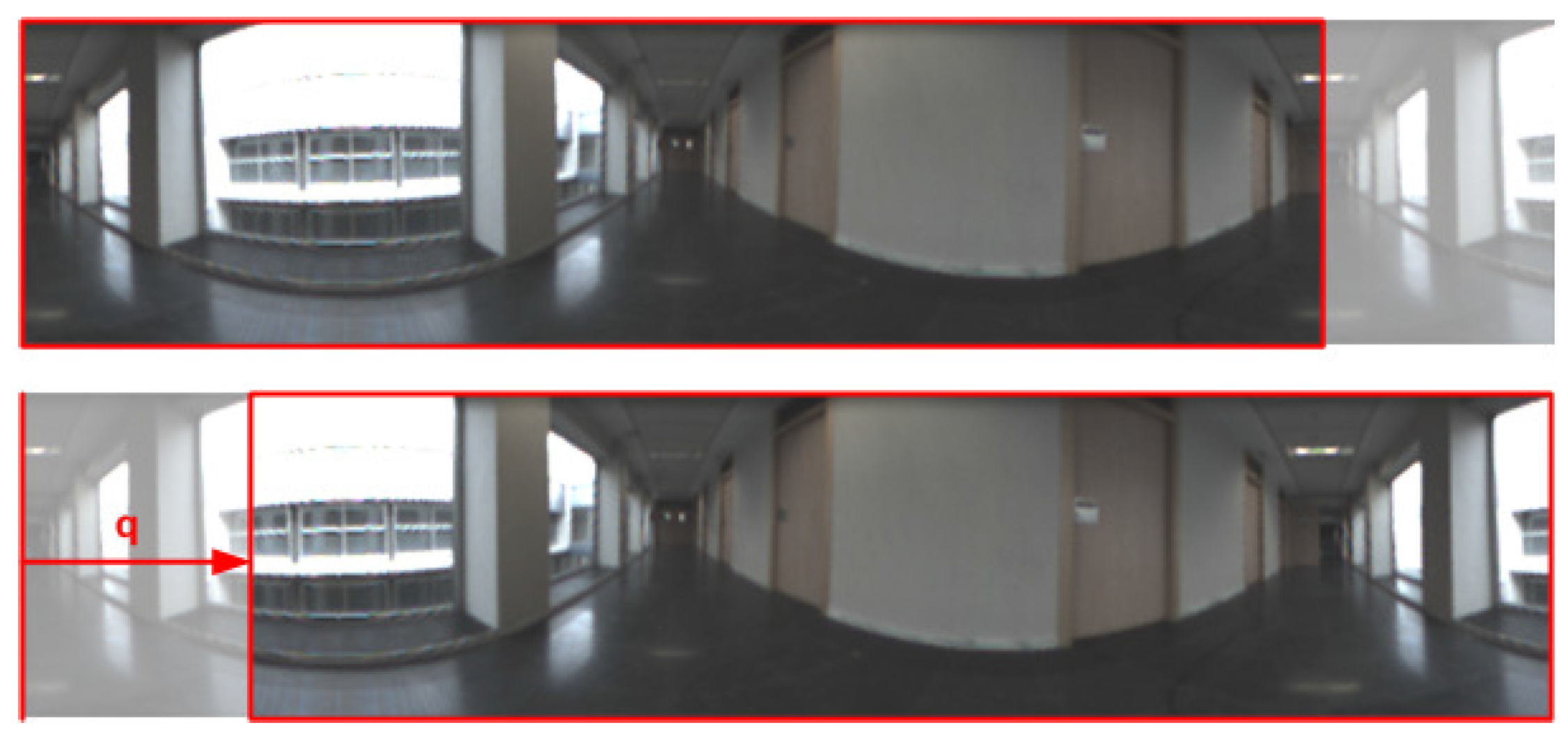
Figure 4.
Set of cells defined in a reference panoramic image for height estimation using the central cell correlation technique.
Figure 4.
Set of cells defined in a reference panoramic image for height estimation using the central cell correlation technique.

Figure 5.
Two panoramic images captured from different heights, to illustrate method 1. (a) Reference image and (b) test image.
Figure 5.
Two panoramic images captured from different heights, to illustrate method 1. (a) Reference image and (b) test image.

Figure 6.
Euclidean distance between the magnitudes matrices of the reference image cells and the test image central cell versus d.
Figure 6.
Euclidean distance between the magnitudes matrices of the reference image cells and the test image central cell versus d.

Figure 7.
(a) Original panoramic image and (b) resulting image after considering a circular shift of rows equivalent to deg.
Figure 7.
(a) Original panoramic image and (b) resulting image after considering a circular shift of rows equivalent to deg.
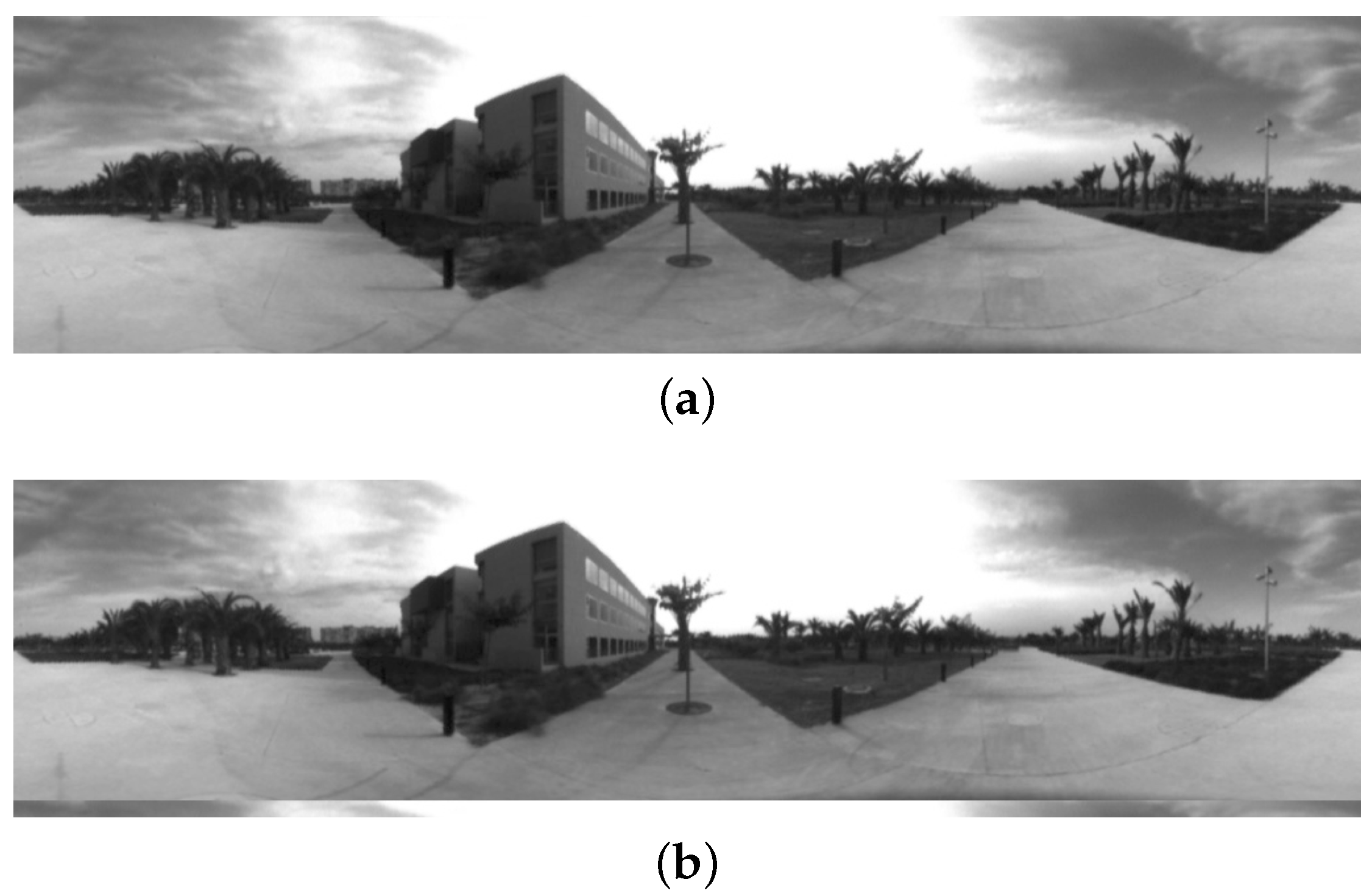
Figure 8.
(a) Original omnidirectional image and (b), (c), (d) three of its orthographic projections considering different focal distances
Figure 8.
(a) Original omnidirectional image and (b), (c), (d) three of its orthographic projections considering different focal distances
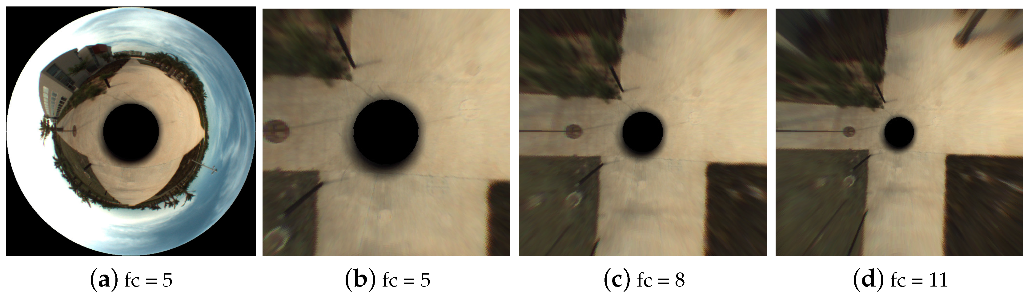
Figure 9.
(a) Projection of a world point P onto the image plane before and after the simulated vertical movement and (b) omnidirectional images and their panoramic projections considering the two different CRS positions.
Figure 9.
(a) Projection of a world point P onto the image plane before and after the simulated vertical movement and (b) omnidirectional images and their panoramic projections considering the two different CRS positions.

Figure 10.
SURF points matched in two images captured with a different relative height (a) with no constraint and (b) searching a match only along the radial line.
Figure 10.
SURF points matched in two images captured with a different relative height (a) with no constraint and (b) searching a match only along the radial line.

Figure 11.
(a) Hyperbolic mirror, (b) Color CCD Camera and (c) tripod.

Figure 12.
Bird’s eye view of the positions above which each set of images was captured (a) outdoors and (b) indoors.
Figure 12.
Bird’s eye view of the positions above which each set of images was captured (a) outdoors and (b) indoors.

Figure 13.
Sample omnidirectional images captured outdoors from three different locations varying the relative position to buildings and lighting conditions. (a) Location 8, (b) location 3 and (c) location 6.
Figure 13.
Sample omnidirectional images captured outdoors from three different locations varying the relative position to buildings and lighting conditions. (a) Location 8, (b) location 3 and (c) location 6.
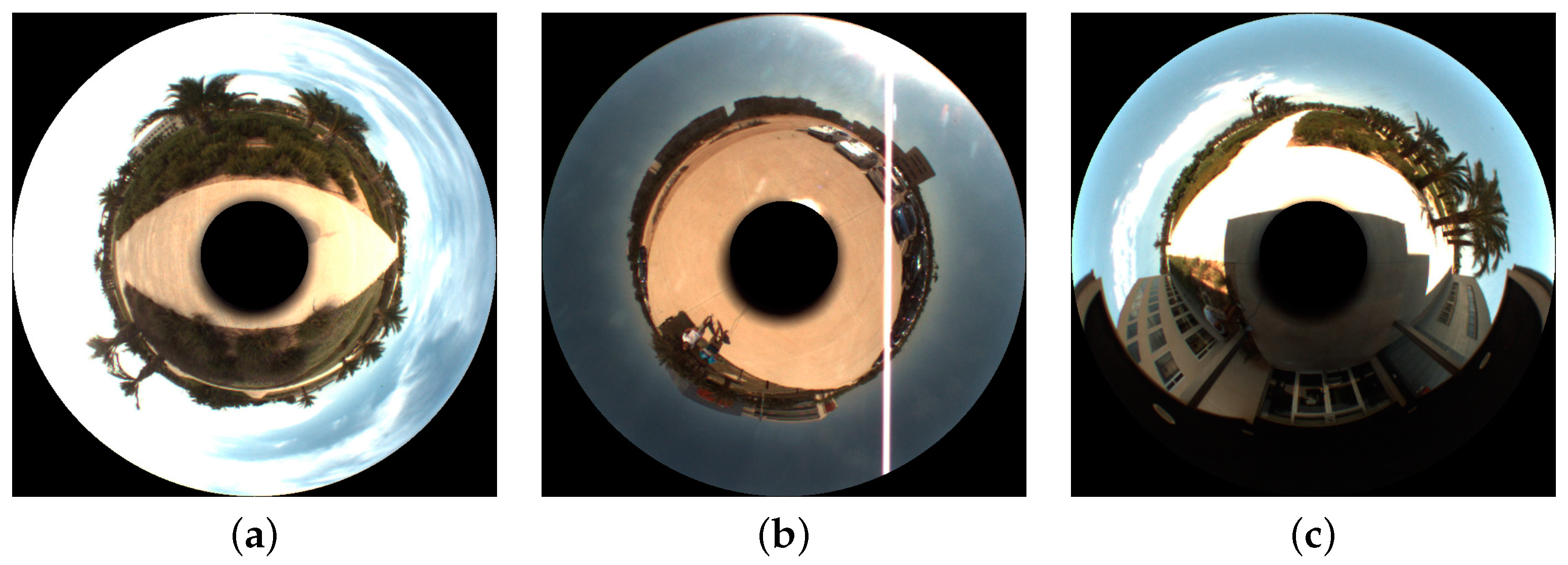
Figure 14.
Sample omnidirectional images captured indoors, in three different rooms. (a) Location 7, (b) location 10 and (c) location 11.
Figure 14.
Sample omnidirectional images captured indoors, in three different rooms. (a) Location 7, (b) location 10 and (c) location 11.

Figure 15.
Sample omnidirectional images captured indoors, from the same location, varying only the height of the capture points. (a) cm (); (b) cm () and (c) cm ().
Figure 15.
Sample omnidirectional images captured indoors, from the same location, varying only the height of the capture points. (a) cm (); (b) cm () and (c) cm ().
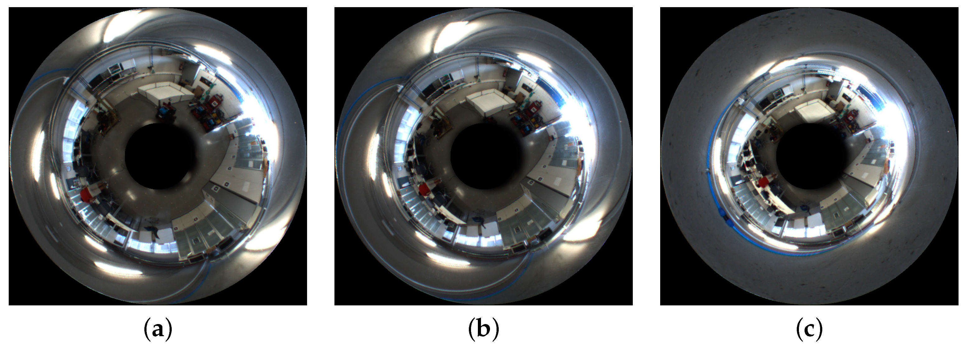
Figure 16.
Results of the experiments in conditions (c1) (blue continuous) and (c2) (green dashed curves), considering all the combinations method-image projection-descriptor shown in Table 3. Outdoor images. (a) Method 1 + Pano. Im. + FS. (b) Method 1 + Pano. Im. + 2D-DFT. (c) Method 2 + Pano. Im. + 2D-DFT. (d) Method 3 + Orthogr. View + FS. (e) Method 3 + Orthogr. View + 2D-DFT. (f) Method 4 + Pano. Im. + FS. (g) Method 4 + Pano. Im. + 2D-DFT. (h) Method 4 + Orthogr. View + FS. (i) Method 4 + Orthogr. View + 2D-DFT. (j) Method 4 + Unit Sphere Proj. + SFT. (k) Method 5 + SURF. (l) Method 5 + SURF + RANSAC.
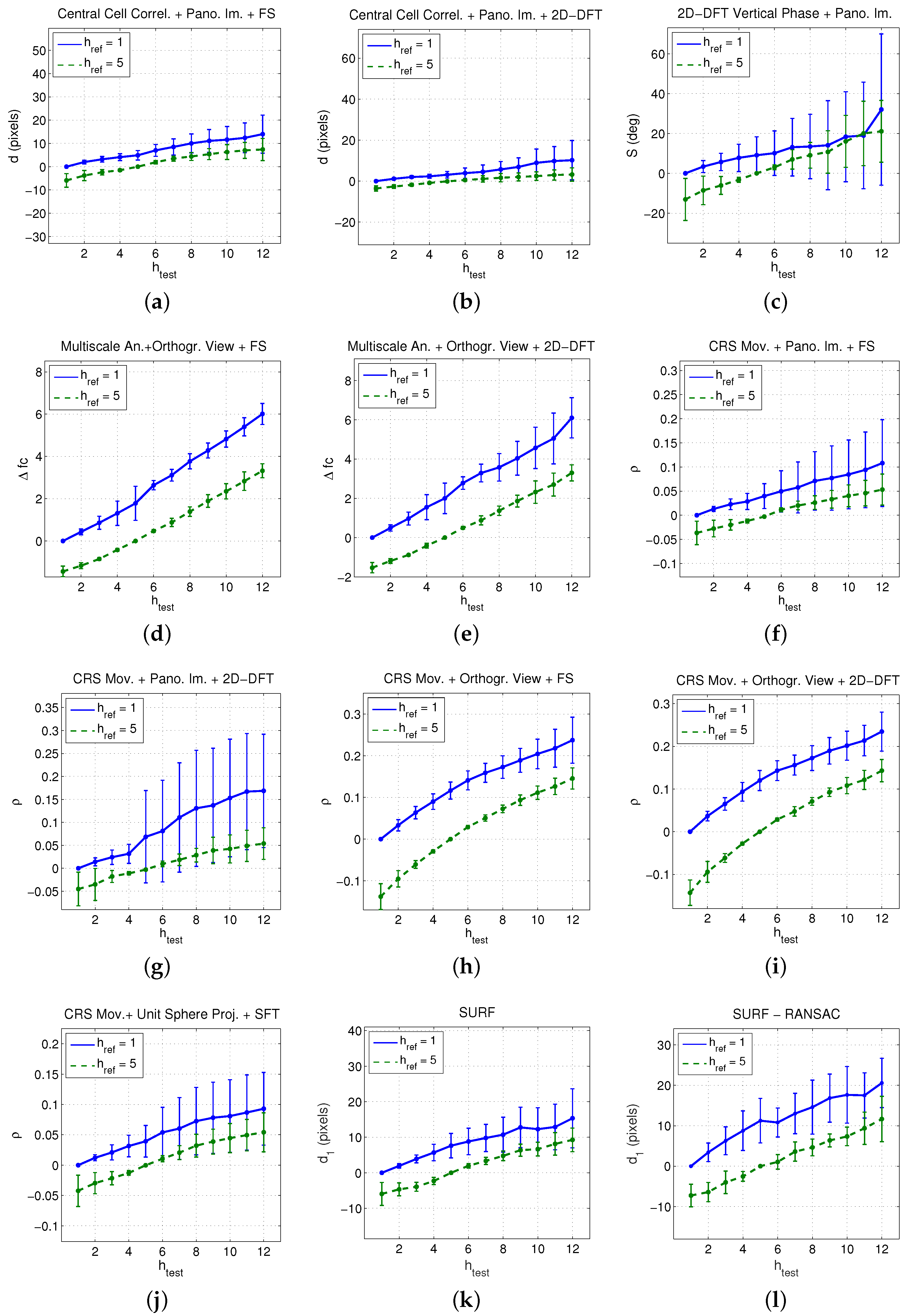
Figure 17.
Results of the experiments in conditions (c1) (blue continuous) and (c2) (green dashed curves), considering all the combinations method-image projection-descriptor shown in Table 3. Indoor images. (a) Method 1 + Pano. Im. + FS. (b) Method 1 + Pano. Im. + 2D-DFT. (c) Method 2 + Pano. Im. + 2D-DFT. (d) Method 3 + Orthogr. View + FS. (e) Method 3 + Orthogr. View + 2D-DFT. (f) Method 4 + Pano. Im. + FS. (g) Method 4 + Pano. Im. + 2D-DFT. (h) Method 4 + Orthogr. View + FS. (i) Method 4 + Orthogr. View + 2D-DFT. (j) Method 4 + Unit Sphere Proj. + SFT. (k) Method 5 + SURF. (l) Method 5 + SURF + RANSAC.
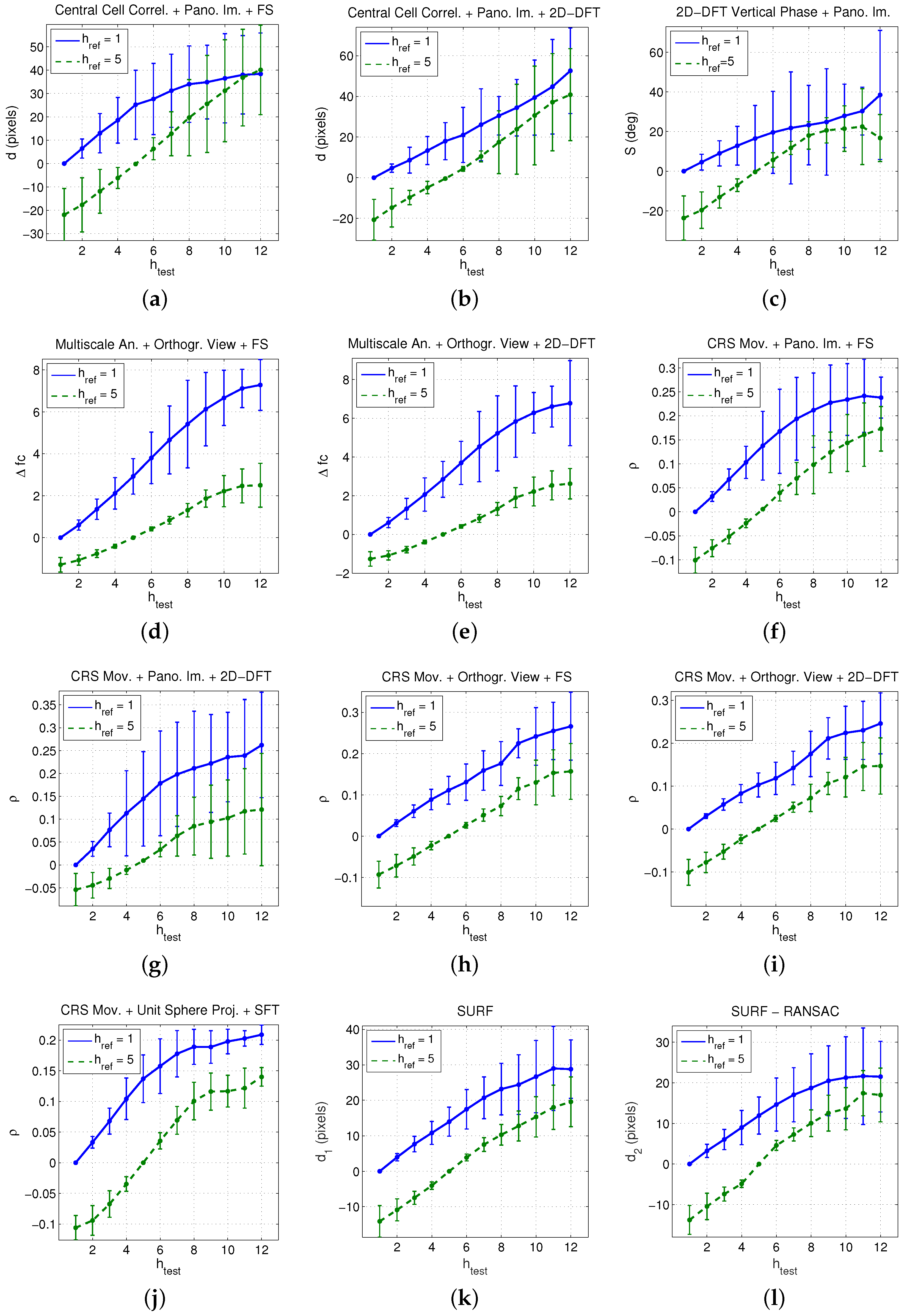
Figure 18.
Variation of the angle of incidence of rays from two points of the environment that are situated at a different distance when the height of the visual system changes.
Figure 18.
Variation of the angle of incidence of rays from two points of the environment that are situated at a different distance when the height of the visual system changes.

Figure 19.
Two sample panoramic scenes captured indoors from different heights. The objects contained in the scenes experience movements with different magnitude.
Figure 19.
Two sample panoramic scenes captured indoors from different heights. The objects contained in the scenes experience movements with different magnitude.

Figure 20.
Results of the experiments in conditions (c3) using outdoor (blue continuous curves) and indoor (green dashed curves) sets of images and considering all the combinations method-image projection-descriptor shown in Table 3. Only positive vertical height gaps are considered in this experiment. (a) Method 1 + Pano. Im. + FS. (b) Method 1 + Pano. Im. + 2D-DFT. (c) Method 2 + Pano. Im. + 2D-DFT. (d) Method 3 + Orthogr. View + FS. (e) Method 3 + Orthogr. View + 2D-DFT. (f) Method 4 + Pano. Im. + FS. (g) Method 4 + Pano. Im. + 2D-DFT. (h) Method 4 + Orthogr. View + FS. (i) Method 4 + Orthogr. View + 2D-DFT. (j) Method 4 + Unit Sphere Proj. + SFT. (k) Method 5 + SURF. (l) Method 5 + SURF + RANSAC.

Figure 21.
Results of the experiments in conditions (c3) using outdoor (blue continuous curves) and indoor (dashed curves) sets of images and considering all the combinations method-image projection-descriptor shown in Table 3. Only negative vertical height gaps are considered in this experiment. (a) Method 1 + Pano. Im. + FS. (b) Method 1 + Pano. Im. + 2D-DFT. (c) Method 2 + Pano. Im. + 2D-DFT. (d) Method 3 + Orthogr. View + FS. (e) Method 3 + Orthogr. View + 2D-DFT. (f) Method 4 + Pano. Im. + FS. (g) Method 4 + Pano. Im. + 2D-DFT. (h) Method 4 + Orthogr. View + FS. (i) Method 4 + Orthogr. View + 2D-DFT. (j) Method 4 + Unit Sphere Proj. + SFT. (k) Method 5 + SURF. (l) Method 5 + SURF + RANSAC.


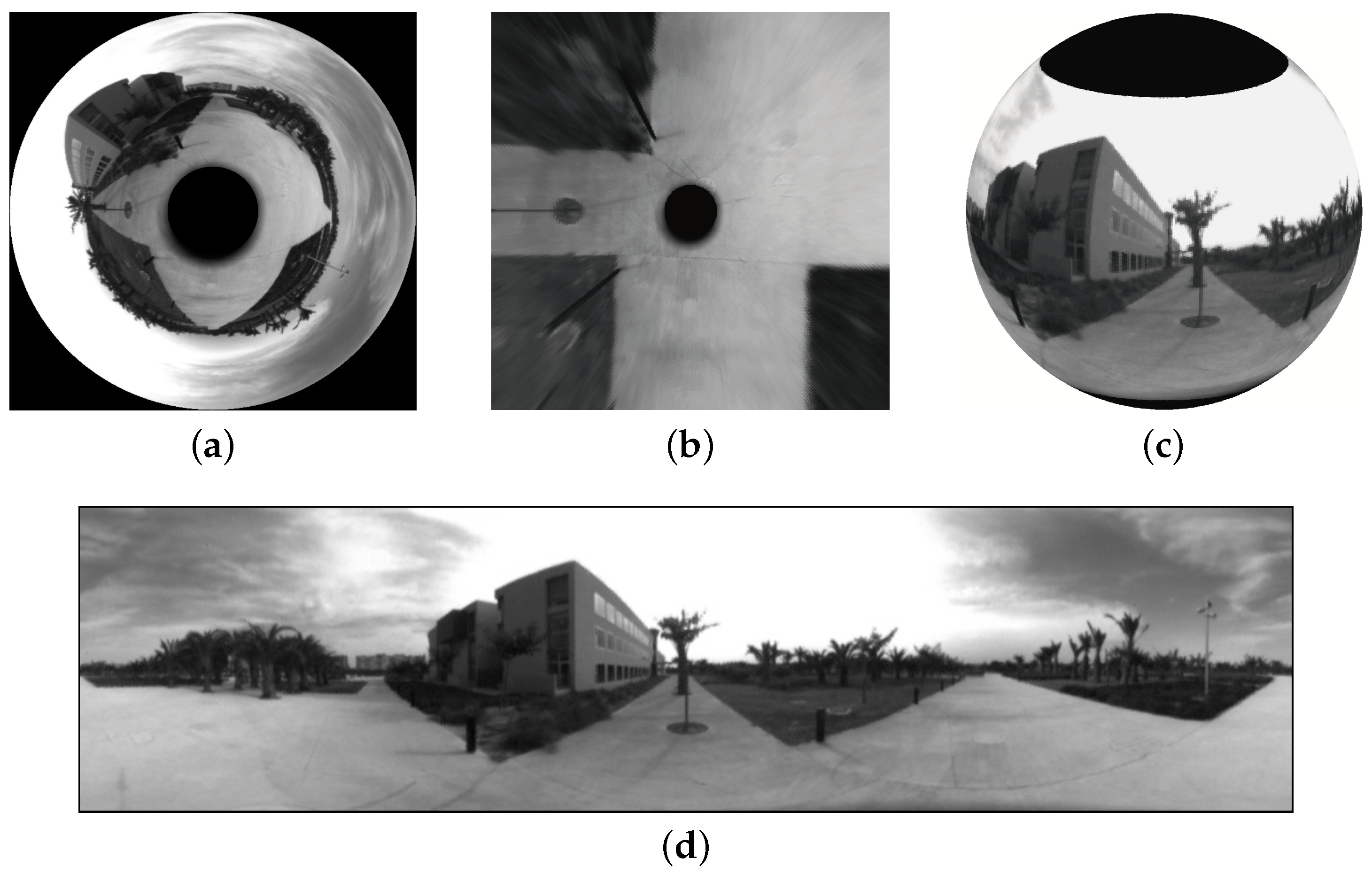
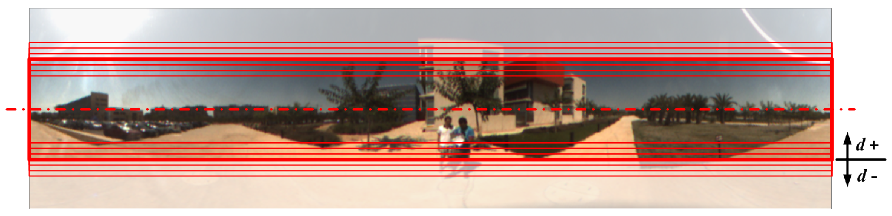
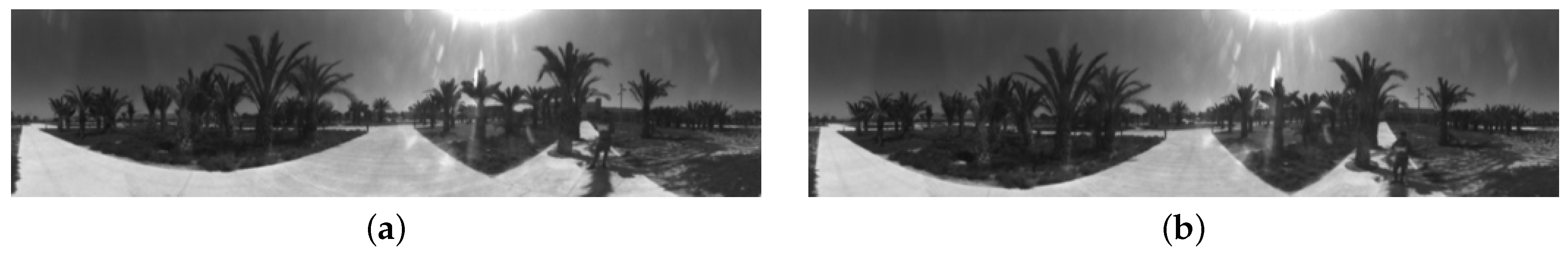
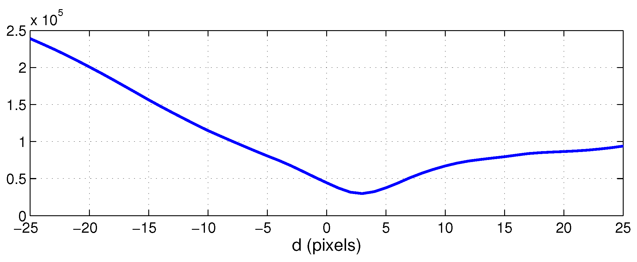
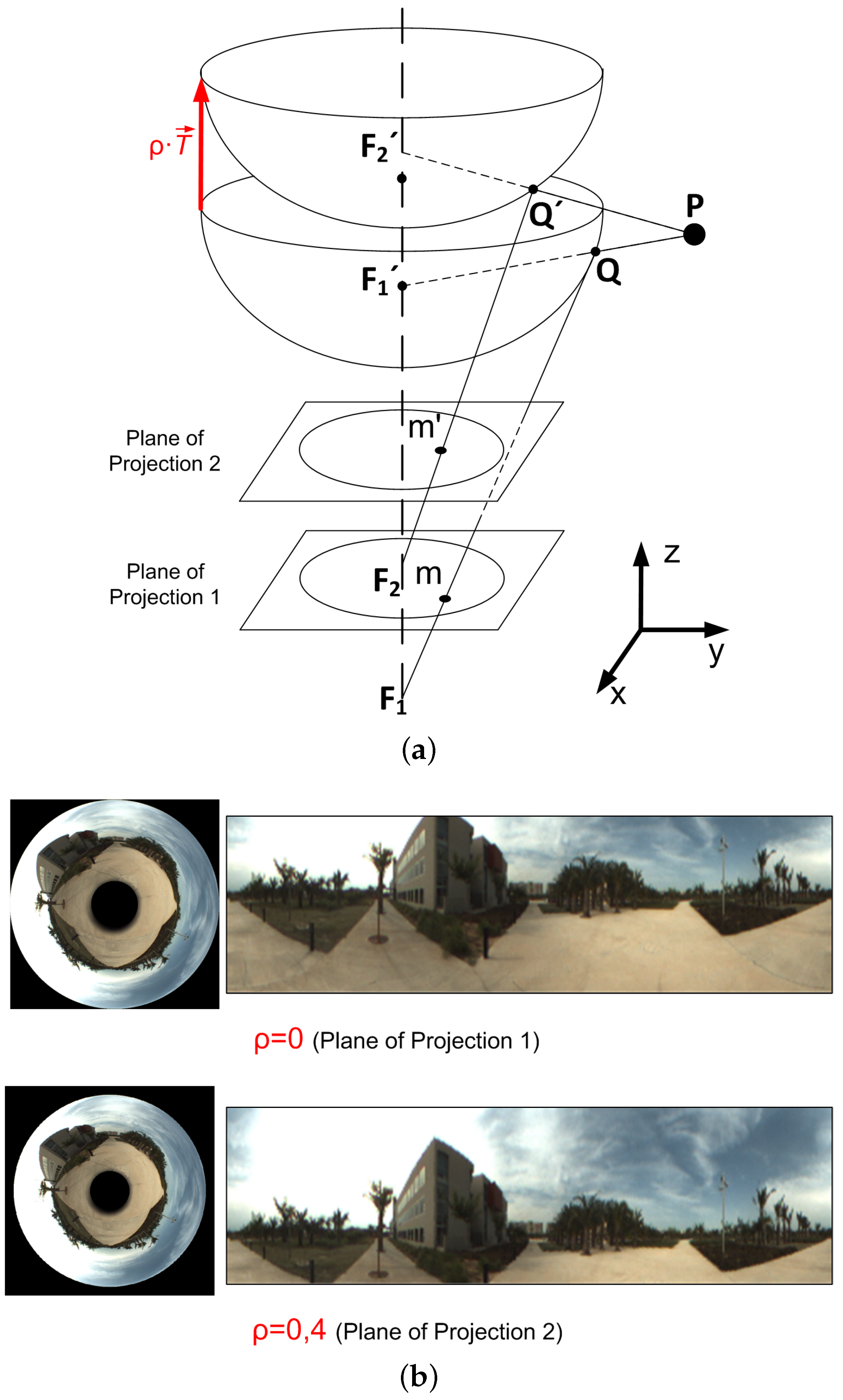
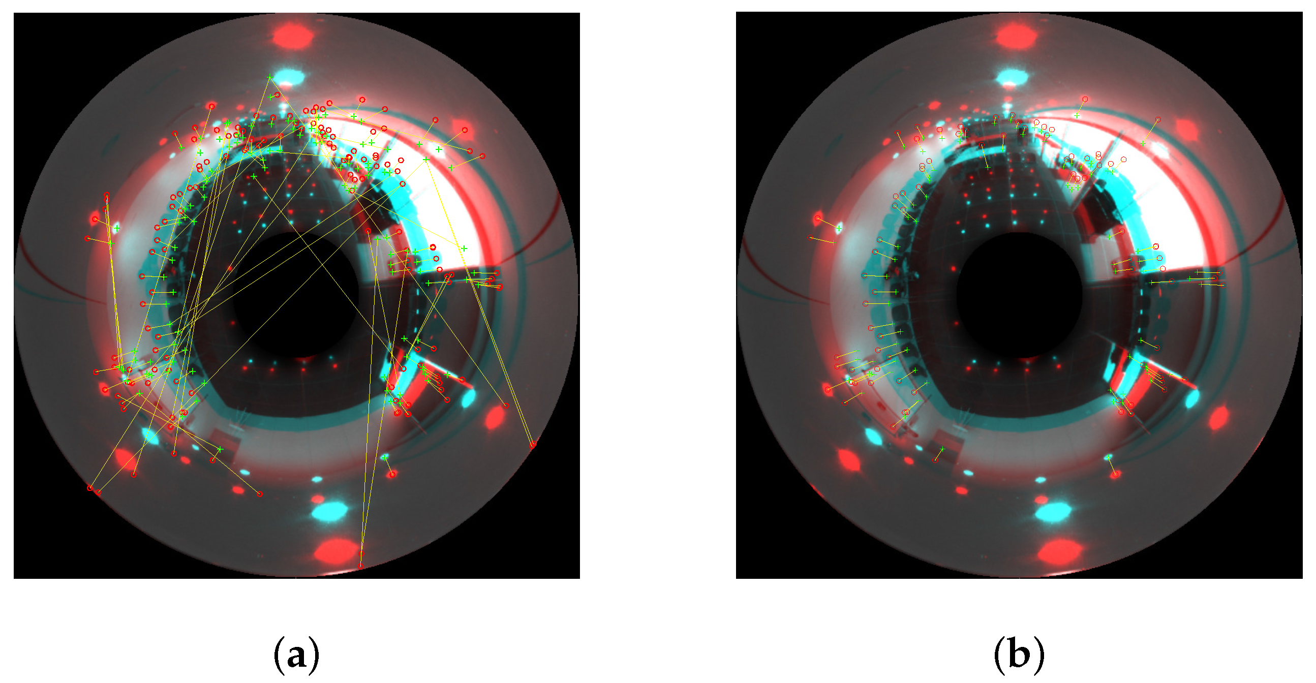
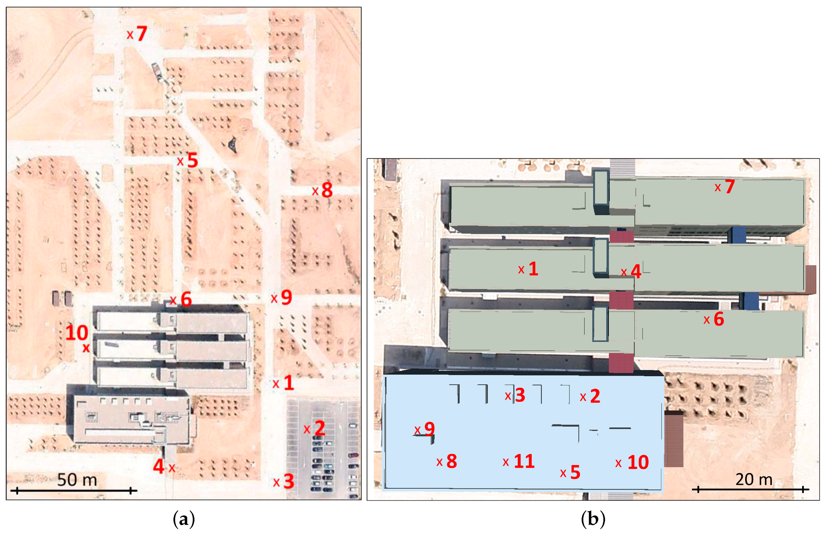
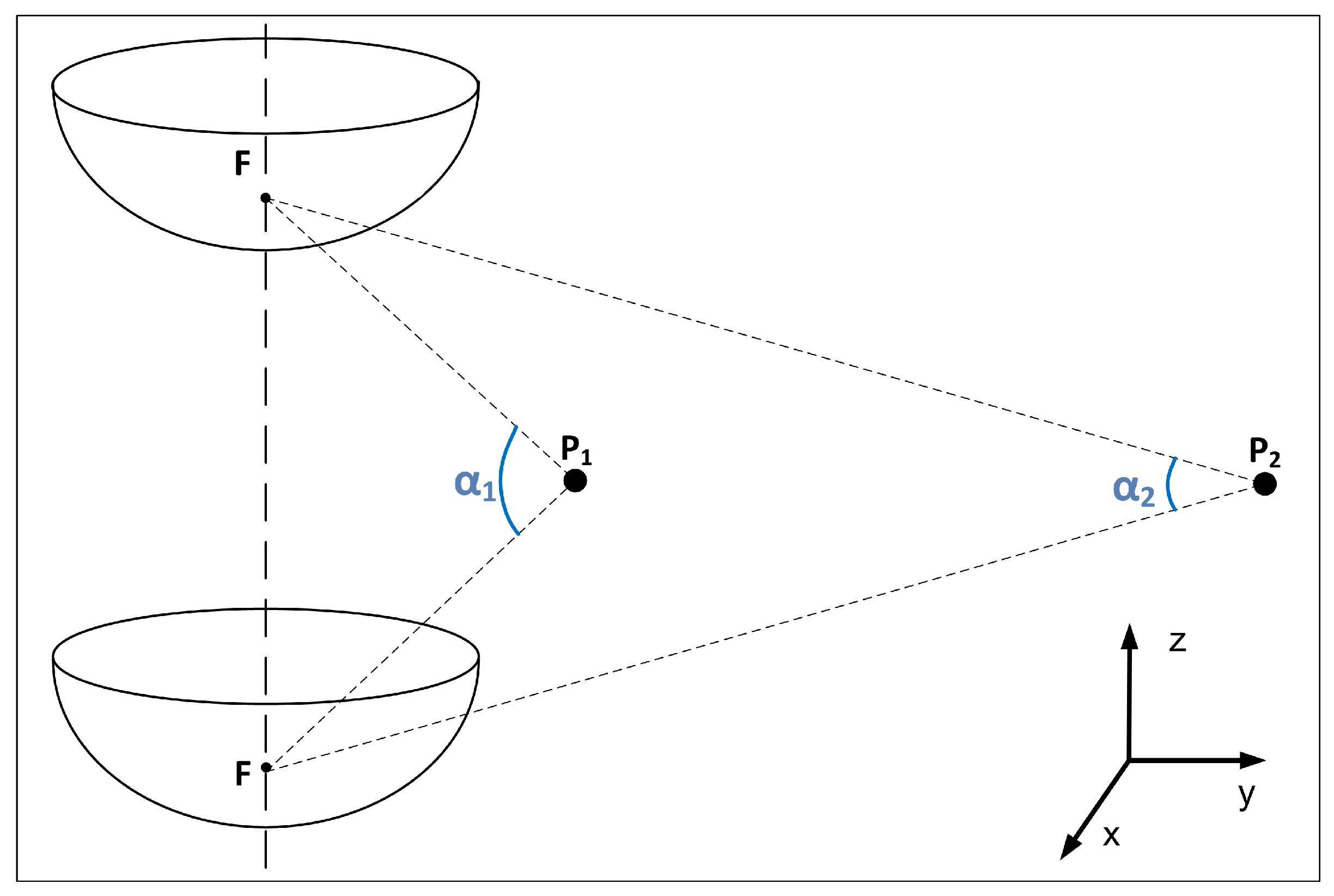
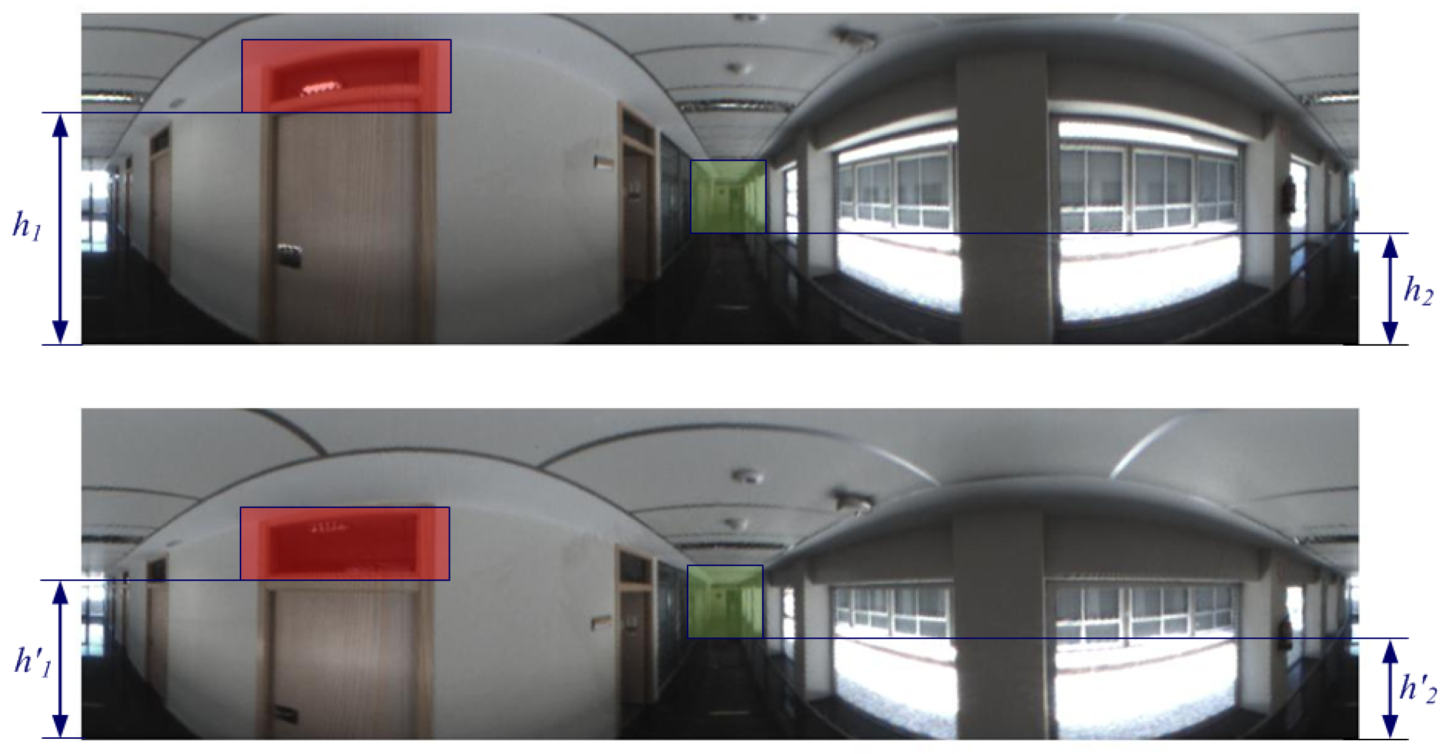
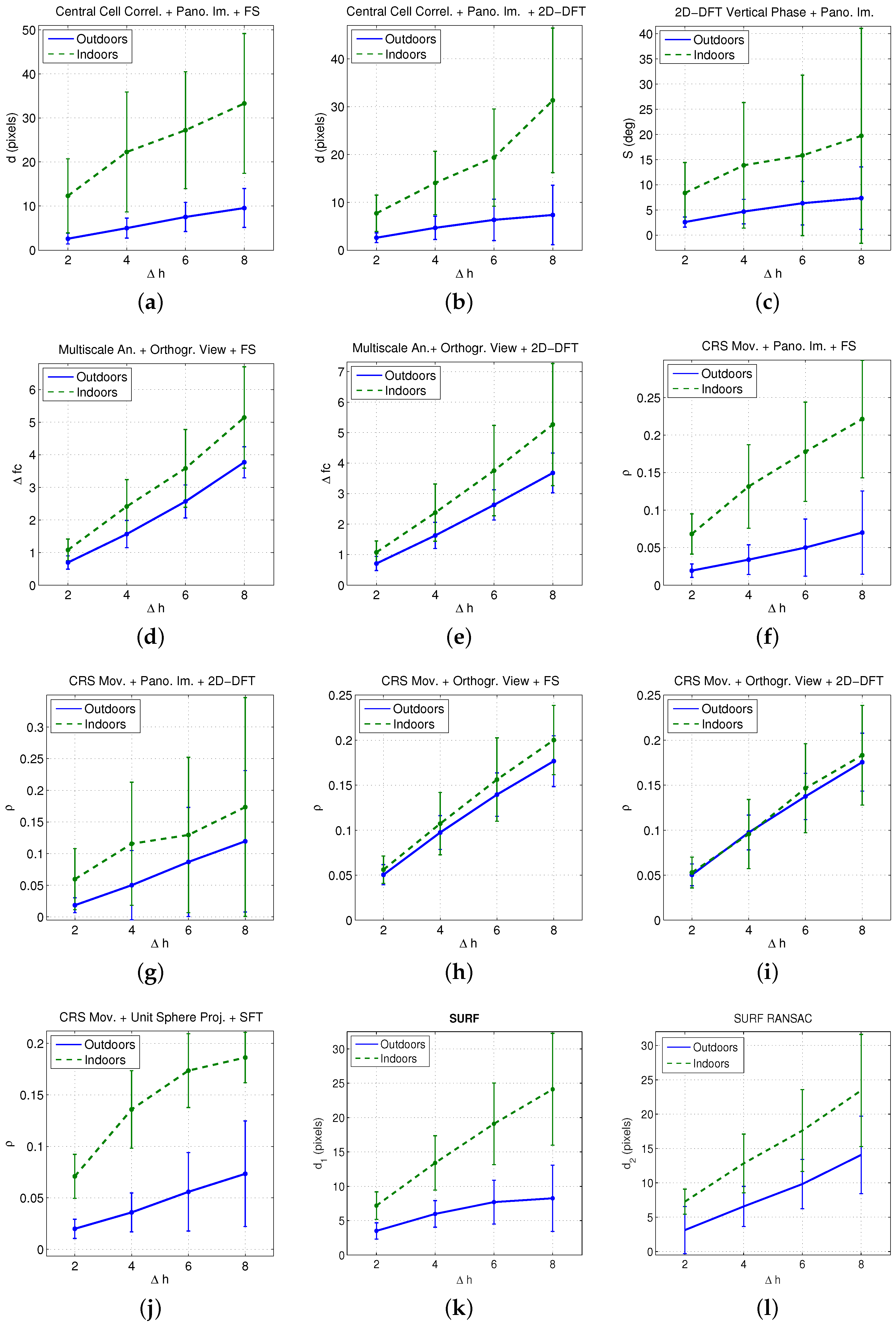
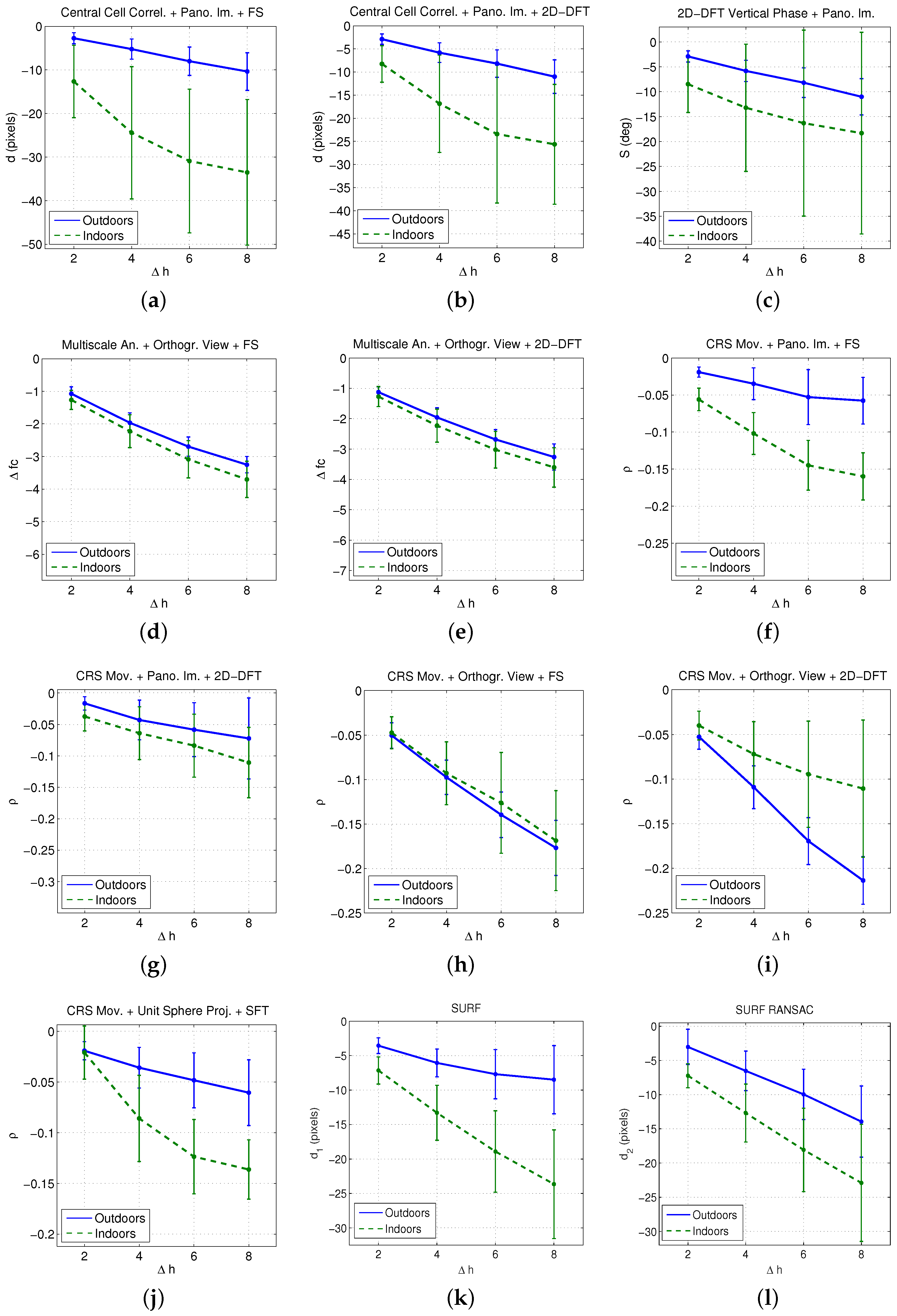
Table 1.
Specifications of the mirror.
| Parameters | Mirror Eizoh Wide 70 |
|---|---|
| Geometry | Hyberbolic |
| Maximum Diameter | 70 mm |
| Height | 35 mm |
| Angle of view above the horizon | 60 deg |
| Angle of view below the horizon | 60 deg |
Table 2.
z-coordinates of the capture points of the sets of images and number of images captured from each z-coordinate.
Table 2.
z-coordinates of the capture points of the sets of images and number of images captured from each z-coordinate.
| h | z (cm) | # Im. Outdoors | # Im. Indoors |
|---|---|---|---|
| 1 | 125 | 10 | 11 |
| 2 | 140 | 10 | 11 |
| 3 | 155 | 10 | 11 |
| 4 | 170 | 10 | 11 |
| 5 | 185 | 10 | 11 |
| 6 | 200 | 10 | 11 |
| 7 | 215 | 10 | 11 |
| 8 | 230 | 10 | 10 |
| 9 | 245 | 10 | 8 |
| 10 | 260 | 10 | 6 |
| 11 | 275 | 10 | 6 |
| 12 | 290 | 10 | 5 |
| TOTAL # IMAGES | 120 | 112 | |
Table 3.
Combinations of height estimation methods, kind of image projection and description method considered to carry out the experiments. The final topological height measurement is also shown.
Table 3.
Combinations of height estimation methods, kind of image projection and description method considered to carry out the experiments. The final topological height measurement is also shown.
| Height Estimation Method | Image Projection | Descriptor | Height Indicator |
|---|---|---|---|
| 1. Central Cell Correlation | Panoramic Image | FS | d (pixels) |
| 2D-DFT | d (pixels) | ||
| 2. 2D-DFT Vertical Phase | Panoramic image | 2D-DFT | S |
| 3. Multiscale Analysis | Orthographic View | FS | |
| 2D-DFT | |||
| 4. Camera Reference System Movement | Panoramic Image | FS | |
| 2D-DFT | |||
| Orthographic View | FS | ||
| 2D-DFT | |||
| Unit Sphere Projection | SFT | ||
| 5. Matching Local Features | Omnidirectional Scene | SURF | |
| SURF-RANSAC |
Table 4.
Configuration of the experiments considered in condition (c3). Height gaps considered and number of experiments for the outdoor and indoor sets of images.
Table 4.
Configuration of the experiments considered in condition (c3). Height gaps considered and number of experiments for the outdoor and indoor sets of images.
| () | # Experiments Outdoors | # Experiments Indoors | |
|---|---|---|---|
| 2 | 30 | 100 | 90 |
| 4 | 60 | 80 | 68 |
| 6 | 90 | 60 | 46 |
| 8 | 120 | 40 | 25 |
Table 5.
Computational cost to describe a reference image, and to describe a test image and estimate its relative height, .
Table 5.
Computational cost to describe a reference image, and to describe a test image and estimate its relative height, .
| Height Estimation Method | Image projection | Descriptor | (s) | (s) |
|---|---|---|---|---|
| 1. Central Cell Correlation | Panoramic Image | FS | 0.0450 | 0.0011 |
| Panoramic Image | 2D-DFT | 0.0709 | 0.0017 | |
| 2. 2D-DFT Vertical Phase | Panoramic Image | 2D-DFT | 0.0032 | 0.0662 |
| 3. Multiscale Analysis | Orthographic View | FS | 11.5117 | 0.1908 |
| 2D-DFT | 10.6323 | 0.1800 | ||
| 4. Camera Reference System Movement | Panoramic Image | FS | 11.8509 | 0.0405 |
| 2D-DFT | 11.3911 | 0.0385 | ||
| Orthographic View | FS | 11.6408 | 0.0273 | |
| 2D-DFT | 11.3409 | 0.0241 | ||
| Unit Sphere Proj. | SFT | 17.8813 | 0.2985 | |
| 5. Matching Local Features | Omnidirectional Scene | SURF | 0.0939 | 0.2354 |
| SURF-RANSAC | 0.0978 | 0.3810 |
Table 6.
Necessary memory to store all the necessary information from a reference image, , and to store the information from a test image, .
Table 6.
Necessary memory to store all the necessary information from a reference image, , and to store the information from a test image, .
| Height Estimation Method | Image Projection | Descriptor | (KB) | (KB) |
|---|---|---|---|---|
| 1. Central Cell Correlation | Panoramic Image | FS | 1312 | 32 |
| 2D-DFT | 328 | 8 | ||
| 2. 2D-DFT Vertical Phase | Panoramic Image | 2D-DFT | 8 | 8 |
| 3. Multiscale Analysis | Orthographic View | FS | 3904 | 64 |
| 2D-DFT | 488 | 8 | ||
| 4. Camera Reference System Movement | Panoramic Image | FS | 1296 | 16 |
| 2D-DFT | 162 | 8 | ||
| Orthographic View | FS | 2496 | 64 | |
| 2D-DFT | 312 | 8 | ||
| Unit Sphere Proj. | SFT | 1952 | 64 | |
| 5. Matching Local Features | Omnidirectional Scene | SURF | 99 | 99 |
| SURF-RANSAC | 99 | 99 |
© 2017 by the authors. Licensee MDPI, Basel, Switzerland. This article is an open access article distributed under the terms and conditions of the Creative Commons Attribution (CC BY) license (http://creativecommons.org/licenses/by/4.0/).
Share and Cite
MDPI and ACS Style
Amorós, F.; Payá, L.; Ballesta, M.; Reinoso, O. Development of Height Indicators using Omnidirectional Images and Global Appearance Descriptors. Appl. Sci. 2017, 7, 482. https://doi.org/10.3390/app7050482
AMA Style
Amorós F, Payá L, Ballesta M, Reinoso O. Development of Height Indicators using Omnidirectional Images and Global Appearance Descriptors. Applied Sciences. 2017; 7(5):482. https://doi.org/10.3390/app7050482
Chicago/Turabian StyleAmorós, Francisco, Luis Payá, Mónica Ballesta, and Oscar Reinoso. 2017. "Development of Height Indicators using Omnidirectional Images and Global Appearance Descriptors" Applied Sciences 7, no. 5: 482. https://doi.org/10.3390/app7050482
Note that from the first issue of 2016, this journal uses article numbers instead of page numbers. See further details here.