
An Efficient Compensation Method for Limited-View Photoacoustic Imaging Reconstruction Based on Gerchberg–Papoulis Extrapolation

1
Department of Electronic Engineering, Fudan University, No. 220 Handan Road, Shanghai 200433, China
2
Key Laboratory of Medical Imaging Computing and Computer Assisted Intervention (MICCAI) of Shanghai, Fudan University, Shanghai 200433, China
*
Author to whom correspondence should be addressed.
Appl. Sci. 2017, 7(5), 505; https://doi.org/10.3390/app7050505
Submission received: 29 March 2017
/
Revised: 8 May 2017
/
Accepted: 9 May 2017
/
Published: 17 May 2017
(This article belongs to the Special Issue Biomedical Photoacoustic and Thermoacoustic Imaging)
Abstract
:The reconstruction for limited-view scanning, though often the case in practice, has remained a difficult issue for photoacoustic imaging (PAI). The incompleteness of sampling data will cause serious artifacts and fuzziness in those missing views and it will heavily affect the quality of the image. To solve the problem of limited-view PAI, a compensation method based on the Gerchberg–Papoulis (GP) extrapolation is applied into PAI. Based on the known data, missing detectors elements are estimated and the image in the missing views is then compensated using the Fast Fourier Transform (FFT). To accelerate the convergence speed of the algorithm, the total variation (TV)-based iterative algorithm is incorporated into the GP extrapolation-based FFT-utilized compensation method (TV-GPEF). The effective variable splitting and Barzilai–Borwein based method is adopted to solve the optimization problem. Simulations and in vitro experiments for both limited-angle circular scanning and straight-line scanning are conducted to validate the proposed algorithm. Results show that the proposed algorithm can greatly suppress the artifacts caused by the missing views and enhance the edges and the details of the image. It can be indicated that the proposed TV-GPEF algorithm is efficient for limited-view PAI.
1. Introduction
Photoacoustic imaging (PAI), also known as optoacoustic tomography, is a novel biomedical imaging technique. It uses laser as the energy source and detects the excited ultrasound signals. Therefore, it combines the advantages of both the ultrasound imaging and the optical imaging [1,2,3]. Firstly, PAI inherits the advantage of the optical imaging’s high contrast [1]. Secondly, it breaks through the imaging depth limitation of the optical imaging and can acquire an image at higher imaging depth with ideal resolution [3]. Thirdly, PAI is also a noninvasive imaging technique that is harmless to the tissue as long as the energy of laser is controlled. Furthermore, because PAI reflects the light absorption distributions of the tissue, it can indicate such physiological parameters as hemoglobin concentration and blood oxygen saturation [4,5,6]. With all these above-mentioned advantages, PAI serves as a great tool in many fields of biomedical application, e.g., brain imaging [7,8], blood vessel imaging [9], tumor detection [10] and molecular imaging [11].
Currently, there are two kinds of PAI: computed-tomography PAI [12,13] and photoacoustic microscope [14,15]. This paper focuses on the computed-tomography PAI. Under these circumstances, the tissue is irradiated by laser uniformly followed by photoacoustic signals generated through the photoacoustic effect [1,2,3] and then the photoacoustic signals are detected by a transducer array or by an ultrasound transducer scanning around the tissue. The collected signals contain the light absorption property information of the tissue. Therefore, the optical absorption distribution of the tissue can be reconstructed by a certain image reconstruction algorithm. In this process, the photoacoustic image reconstruction algorithms play a significant role in ensuring the quality of the reconstructed images.
Since the initial study, many efforts have been made for the development of the photoacoustic image reconstruction algorithms. Analytical reconstruction algorithms are the first kind of photoacoustic image reconstruction algorithms [16,17,18,19,20]. In 1995, Kruger et al. proposed the first photoacoustic image reconstruction algorithm by using the inverse Radon transform [16]. After that, the filtered back-projection method (FBP) proposed by Xu et al. was the most popular reconstruction algorithm for PAI [18,21,22,23,24]. Mohajerani et al. proposed a fast Fourier backprojection-based algorithm to solve the photoacoustic equation in frequency domain [17]. The deconvolution reconstruction algorithm proposed by Zhang et al. utilized the deconvolution-based method to improve the results of both full-view and limited-view scanning [20]. The advantage of the analytical reconstruction algorithms lies in its fastness and concision. However, they have poor accuracy and high dependence on data. To overcome the shortcomings of the analytical reconstruction algorithms, the iterative reconstruction algorithms which set up a forward model from the photoacoustic signals to the image have been applied into PAI and have obtained excellent results [25,26]. This kind of reconstruction method is also called model-based photoacoustic [27]. Paltauf et al. proposed an iterative reconstruction algorithm for optoacoustic imaging [26]. Huang et al. incorporated the full-wave mode into the iterative reconstruction algorithm to effectively solve the problem caused by the inhomogeneities of the sound speed [25]. The compressed sensing theory was also applied in the photoacoustic image reconstruction algorithms [28,29,30,31]. Among the iterative algorithms, total variation-based (TV) algorithms are reported to work best [32,33,34]. Zhang et al. proposed a gradient descent-based TV (TV-GD) algorithm which has greatly improved the reconstruction results, especially in sparse-view sampling [34]. Arridge et al. proposed a TV-based Bregman iteration to effectively solve the PAI sub-sampling problem [32].
Under the circumstance of full-view scanning, most existing photoacoustic image reconstruction algorithms are capable to get satisfactory results. In practice, however, it is often the case that the acquired data does not meet the condition of data completeness due to the restriction of many physical conditions such as human body shape, anatomical position, light exposure and data detection time. For the limited-view scanning where only incomplete sampling data can be acquired, many reconstruction algorithms fail to perform well [34,35,36,37]. There are mainly two types of scan patterns for limited-view PAI: limited-angle circular scanning and straight-line scanning. Besides, some irregular scanning with unclosed scanning curves also belongs to limited-view scanning. The reconstruction for the limited-view has always been a difficult issue for PAI. Since the angle range of the projection cannot meet the data integrity conditions, severe stripped artifacts appear and details of the image are seriously affected [35,37]. Although traditional iterative reconstruction algorithms such as TV based algorithms can substantially reduce the number of measured angles required, lack of some angular projection data will lead to such problems as blurring image edges and obvious artifacts, which will seriously affect the quality of the reconstruction images especially when data is seriously inadequate [38,39,40,41]. It is reported that, in the case of limited-view scanning, reconstruction algorithms for PAI (e.g., the iterative adaptive weighted FBP method proposed by Liu et al. [42]) can improve their performance, but problems such as the severe dependence on the data and obvious artifacts still remain. There is still plenty of room for improvement [42,43]. Other methods improve the results of limited-view PAI by designing more advanced experimental setups [44,45,46]. For example, Huang et al. proposed an improved limited-view PAI method through an acoustic reflector [45]. However, these methods will increase the complexity of the setup as well as the cost of PAI. Therefore, we need to develop a new photoacoustic reconstruction algorithm to further reduce the artifacts while enhancing the image edges and reducing the requirements for the amount as well as the completeness of the data for limited-view PAI.
In this paper, we propose an efficient reconstruction method for limited-view PAI based on the Gerchberg–Papoulis (GP) extrapolation. We incorporate the GP-based extrapolation method [47,48] into the TV-based iterative reconstruction algorithm to compensate for the deficiency of data. For every iteration, the missing detectors are estimated by the reconstructed image obtained in that iteration and the image in those missing angles is back projected by the estimated missing detectors. Then the reconstructed image is compensated by weighted addition to the estimated image in the missing region. By using the fast Fourier transform (FFT) between Fourier space and image space in GP-extrapolation, it can improve the speed and accuracy of the algorithm (GPEF). Then the GPEF method (GP extrapolation method using FFT) is embedded into the TV-based optimization. We use TV-GPEF to stand for this method which incorporates the TV minimization into GPEF method to update each GPEF iteration. We adopt the efficient variable splitting and Barzilai–Borwein based method to solve the constrained TV minimization problem. The reconstruction performances of the proposed TV-GPEF algorithm are compared to those of the TV-GD (TV-based algorithm solved by gradient descent method) and TV-VB (the TV-based algorithm solved by the variable splitting and Barzilai–Borwein based method, the same method as that of TV-GPEF but not compensated by the GP-based method). Numerical simulations and in vitro experiments for both limited-angle circular scanning and straight-line scanning verify the efficiency of the TV-GPEF algorithm and show great improvement over the other two algorithms for limited-view PAI. The artifacts caused by the deficiency of data are well suppressed and edges of the image in those information-missing region are well enhanced. In addition, the peak signal-to-noise rations (PSNR), the noise robustness and the convergence of the algorithms are also discussed and compared.
The main contribution of the paper is that we have developed a novel photoacoustic reconstruction algorithm to effectively solve the problem of limited-view PAI. Firstly, by incorporating the GP-extrapolation based method into PAI iterative reconstruction algorithm, excellent results for the compensation of the missing data have been obtained. Then, through constraining the GP-based compensation method with the TV-based optimization, the convergence of the algorithm can be improved. Finally, we implement the variable splitting and Barzilai–Borwein based method to solve the TV-based optimization problem and thus to accelerate the convergence speed of the algorithm.
2. Theory and Methods
2.1. Model-Based Photoacoustic
In computed-tomography PAI, we usually use a short laser pulse to vertically and uniformly incident upon the tissue. Then, the energy of the laser is absorbed by the tissue and the initial ultrasound field is inspired through the photoacoustic effect. The generated photoacoustic signals propagate in the medium and are detected by the ultrasound transducer scanning around the tissue. The relationship between the photoacoustic signals and the photoacoustic images could be described by the following equation [3]:
where p(r, t) is the generated acoustic pressure at the position r and the time t, A(r) is the light absorption deposition of the tissue, c is the speed of sound, β is the isobaric expansion coefficient and Cp is the specific heat.
Assuming that the acoustic property of the medium is homogeneous and the laser pulse approximates the delta function, for the two-dimensional case, which is mainly concerned in this paper, Equation (1) can be solved by Green’s function [3]:
where r0 is the position of the transducer.
In the model-based PAI, a forward model is usually established to express the relationship between photoacoustic image and photoacoustic signals in matrix multiplication. From Equation (2), it can be derived that:
Defining the left side of Equation (3) as:
where g(r0, t) is the integral for the sampled signal at r0 multiplied with t.
Then, Equation (3) can be rewritten as:
In a practical reconstruction system, the photoacoustic image and the detected signals usually need to be discretized. The photoacoustic image is discretized to a matrix A with the size of Nx × Ny and g is discretized to the column vector g. From Equation (5), we can see that g is the line integral of A so every element in the vector g can be expressed as the weighted sum of the elements in matrix A and the weight value is related to the position of the integral arc [34]:
where l refers to the number of the sampling point. (*)T means transpose of the matrix. N is total number of the sampling points. A′ is a column vector which is rearranged from A. Wl is the corresponding weight matrix.
As a method of the compressed sensing, the TV measures the local variation of an image which can be expressed as the L1 norm of the discrete gradient-matrix of the image [49]:
where Ai,j is the gray value of the image at the pixel (i,j).
When TV is incorporated into the iterative reconstruction method, the optimization problem of the TV-based photoacoutic model-based reconstruction method can be expressed as:
Define the finite difference which approximates to the gradient of A at the kth pixel as: uk = DkA, Equation (8) can be written as:
2.2. GPEF Compensation Method
The GP extrapolation was firstly proposed by Gerchberg and Papoulis as a new method to calculate the Fourier transform of a band-limited function [47,48]. It is executed by means of the FFT between Fourier space and image space and thus improve the accuracy and the speed of the algorithm [50]. The GPEF method to compensate for the limited-view of PAI is demonstrated as the following equation:
where An is the obtained image in the nth iteration. η is the relax factor which is between 0 to 1. MS and MI are the operators that express the regions of the corresponding missing views to the signals and image, respectively. is the corresponding region of missing views of the image A calculated from MIAn in image space. MS and MI are defined as:
where S represents the support of the position of the missing detectors which need to be estimated. I represents the support of missing views of the image, to be blurred during the reconstruction and need to be compensated. Xu et al. in [38] had described the general rule for finding the “detection region” as well as “invisible region” in detail. As it was said in [38], the parts of the boundaries’ normal lines to which pass through a detector position can be stably recoverable. This region is the measured region or the known. While the complement forms the invisible part that is the missing views I in the manuscript. This region is to be blurred during the reconstruction and need to be compensated. S denotes the positions of the missing detectors which is in the projection space. S is chosen to make sure that all the normal lines of the boundaries pass through a detector position so that all the images can be reconstructed stably. L and L−1 denote the operator of the forward and backward projection between signals and the image which is conducted using the FFT in frequency domain based on the following relationship [51]:
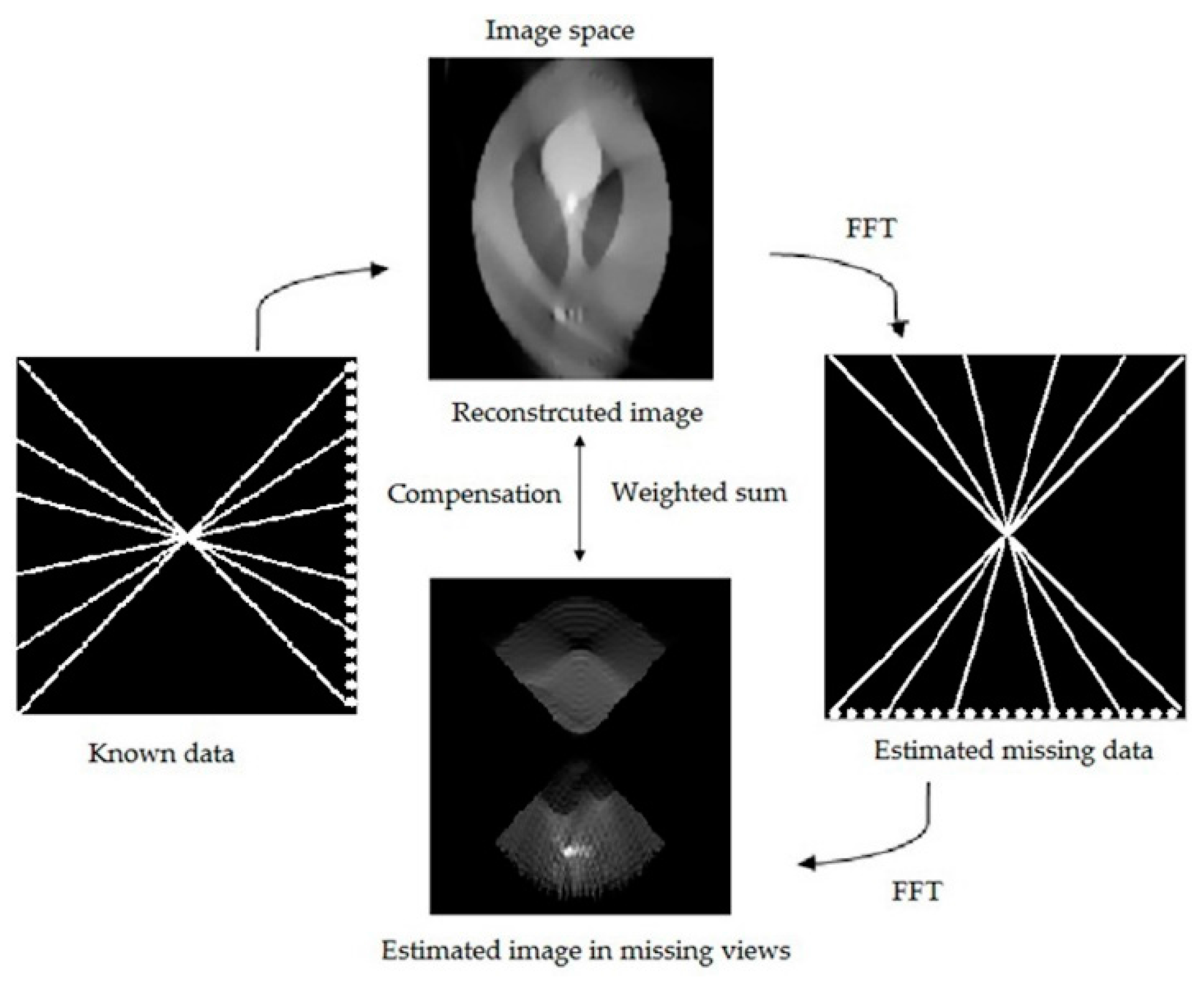
where is the Fourier transform of the photoacoustic image A(i,j). is the Fourier transform of photoacoustic signal p(i,j,t). Implementing Equation (14) requires the following steps: (1) Fourier transform the photoacoustic signal p(i,j,t) to obtain ; (2) use the relationship in Equation (14) to obtain ; and (3) inverse Fourier transform to reconstruct the photoacoustic image A(i,j). The diagram of the Gerchberg-Papoulis-based compensation method is displayed in Figure 1.
The main idea of the GP algorithm is that it compensates for missing data via extrapolations between two spaces. The extrapolations in GP are carried out using FFT so that it is between signal space and Fourier space. As can be seen in Equations (10) and (11), during the iteration, missing detector elements are estimated from MsLAn in the Fourier space. Then, the missing views of A usually blurred by the artifacts are estimated by the missing detectors and compensated by weighted addition to this part of re-estimated image. Implementing the extrapolation in the frequency domain will guarantee the speed and accuracy of the compensation method.
2.3. TV-GPEF Algorithm
The convergence of the GP-type extrapolation has been theoretically proven. However, the pure application of the GP-type extrapolation to compensate for the loss caused by the data deficiency is still not stable in practical for its weak noise robustness and frequent oscillations. Therefore, we combine the GPEF compensation method with the TV-based optimization to improve the stableness and the convergence of the algorithm.
The variable splitting and Barzilai–Borwein based method is implemented to solve the optimization problem [52]. This method is known to have excellent performance in resolving the TV-based minimization problem. The optimization problem for the TV-based algorithm in Equation (9) can be rewritten as:
where α and λ are weights of two parts of the objective function.
By using the standard augmented Lagrangian method and incorporating the Barzilai–Borwein step size to obtain faster convergence [52,53], the problem of Equation (15) can also be deduced as:
where is the defined step parameter for the TV in the nth iteration and δn is the defined Barzilai–Borwein step size in the nth iteration. The updating of δn can be determined by the Barzilai–Borwein method. After using the variable splitting method, Equation (16) can be transformed into the following two sub-problems [41,52]:
The two sub-problems can be solved as follows using the shrinkage operator method [41,52]:
where F is the Fourier transform matrix.
We apply the TV-based algorithm into the GPEF compensation method. In every iteration, the image is first updated by the TV optimization and then compensated by the GPEF method. The iteration steps of the TV-GPEF algorithm are summarized as follows:
- Initialization: Input A, α, λ, η. Set δ0 = 1, b0 = 0. Determine MS and MI according to the scan patterns of the reconstruction based on the rule in [38] as is mentioned above.
- Update un using Equation (18) for the given An−1’. Update An using Equation (19) for the given un. Update bn and δn using Equation (17).
- Input the image An to Equations (10) and (11) to obtain the compensated image in the nth iteration An’.
- If the terminal condition is met, end the iteration. Otherwise, n = n + 1 and return to Steps 2 and 3. The exiting condition is as follows:
3. Simulation Results
In order to validate the proposed TV–GPEF algorithm, a series of numerical simulations are conducted for limited-view scanning. First, straight-line scanning with different sampling points are carried out for the Sheep–Logan phantom which is a widely used phantom in biomedical imaging. Then, limited-angle circular scanning with varying sampling views is also tested. The reconstruction results for the TV–GPEF algorithm are compared to those of the TV–GD and the TV–VB algorithm quantitatively and qualitatively. The PSNRs of these three algorithms are compared and the noise robustness, the convergence speed of the algorithms are also studied. The simulations are conducted using Matlab R2013a on a personal computer with a 2.4 GHz Intel(R) Xeon® CPU and 64 GB memory. The speed of sound is set to 1500 m/s. The simulations for photoacoustic signals and image reconstruction are all carried out in a two-dimensional plane.
3.1. Straight-Line Scanning
The Sheep–Logan phantom is chosen as the original distribution of the light absorption of the image which is shown in Figure 2. The number of pixels in the image are 128 × 128 corresponding to the simulation area of 76.8 mm × 76.8 mm. The transducer detects the signals from the right side of the phantom. The perpendicular distance from the center of the image to the scanning line is 38 mm. The length of the scanning line is 76 mm which remains unchanged but the numbers of sampling points are varying resulting in different sampling intervals. The diagram of the straight-line scanning is also shown in Figure 2. The simulations with the sampling points of 50, 20 and 10 are executed, respectively. The number of iterations is 10 for all three algorithms. The adaptive tunable parameter for the TV-GD algorithm is set to 2 at first iteration and decreased to 0.2 when iteration number is greater than 10, which, as [34] reported, is the best selection when the iteration time is 10. The parameter settings for the TV-VB and the TV-GPEF are estimated by testing the values that provides the best performance for the simulations. The values of the parameters are set to α = 0.4, λ = 1. η is set to 0.15, 0.10, and 0.07, corresponding to 50, 20, and 10 points sampling. The position of the compensated missing views for the signals and image are also shown in Figure 3. The white region in Figure 3 is the corresponding image region to the missing views corresponding to I defined in Section 2.2. The rule to determine this region is also illustrated in Section 2.2. Because the missing views of the image is to be blurred due to the missing of the detector elements, this part of the image need to be compensated while keep the known part (black area) as is because this part can be stably recovered. The axis labels in Figure 3 are the same as that of the phantom in Figure 2.
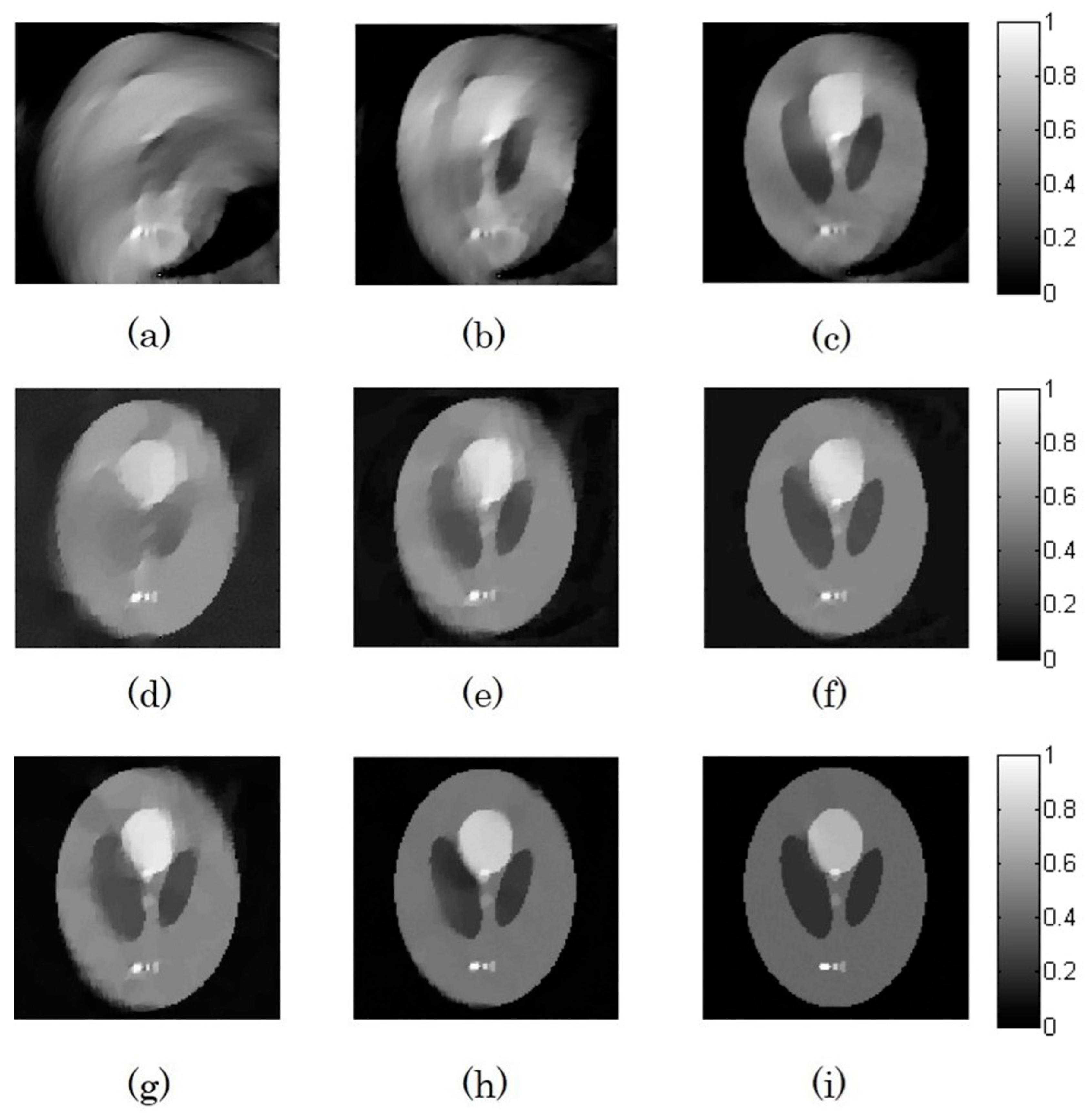
The reconstructed images for three algorithms are shown in Figure 4. It is seen in the first line of Figure 4 that plenty of artifacts exist and blurry edges perpendicularly in the results of the TV-GD on account of the deficiency of data in vertical direction. When the number of sampling data decreases, the blurry phenomenon becomes even more serious and the quality of the image is damaged gravely. It is hard to obtain the useful diagnostic information from the missing views and its application is limited. For the TV-VB algorithm in the second line, due to the efficiency of the Barzilai–Borwein based method, the artifacts caused by the missing views are improved with sufficient sampling points but it has poor results when the sampling points become sparse. As for the TV-GPEF algorithm in the third line, we can see that the results are greatly improved. There are almost no blurs in the reconstructed images and the artifacts are reduced remarkably. Even with sparse sampling points, the degree of vagueness in the missing views is significantly less than those of other two algorithms. Moreover, the contrast of the image is also improved and the background noise is effectively suppressed.
To present the results quantitatively, we also compare the PSNRs of the reconstructed images for these three algorithms. The computation formula of PSNR is as follows:
where MAXI is the maximum gray value of the image. Ri,j is the gray value of the original image. The results of PSNRs are displayed in Table 1. Results show that the TV-GPEF acquires the highest PSNRs compared to those of other two algorithms with the average of 11 dB higher than that of the TV-GD and 7 dB higher than that of the TV-VB. From the results of PSNR, we can see that the TV-GPEF algorithm is superior to the other two algorithms.
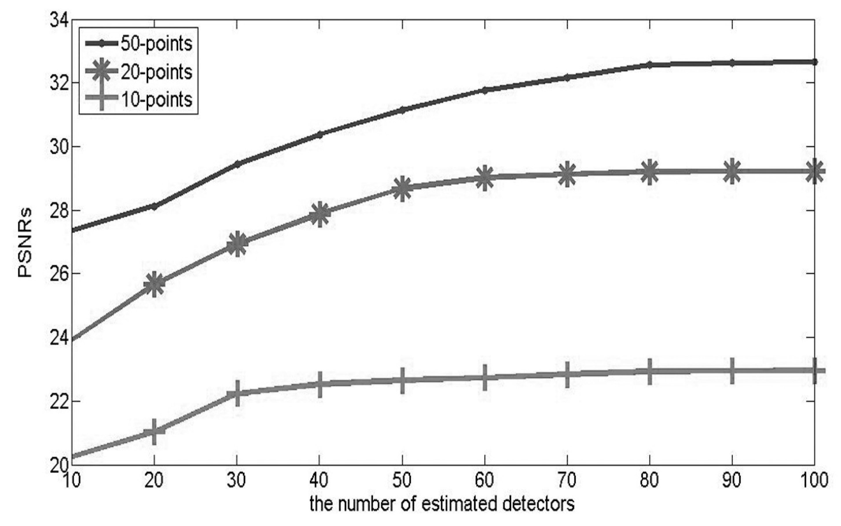
The number of the estimated detectors is another factor which need to consider for TV-GPEF algorithm. We have represented the PSNRs versus the number of estimated detectors for the straight-line scanning in the line chart in Figure 5. It is found that properly increasing the number of estimated detectors elements would improve the results to some extent. However, as the number of estimated detectors continues to increase, the trend of improvement would tend to mitigation. When the increase comes to a certain degree, there would be almost no improvement for the results. Meanwhile, the calculation time would increase greatly. Considering the factors of PSNR and calculation time comprehensively, we choose the number of the estimated detectors of 80, 50, and 30 for 50-points, 20-points and 10-points scanning, respectively.
3.2. Limited-Angle Circular Scanning
Simulations for limited-angle circular scanning are also carried out. In this case, the scanning step of angle remains unchanged, and is set to 6°. The number of the sampling points are set to 10, 15 and 20, respectively, corresponding to 60-views, 90-views and 120-views circular scanning. The radius of the scanning is 36 mm. The values of the parameters are set as α = 0.6, λ = 1. η is set to 0.16, 0.08, 0.05 corresponding to 120-views, 90-views, 60-views scanning. The diagrams of the scanning are shown in Figure 6a–c. Figure 7a–c shows the corresponding areas of compensated missing views.
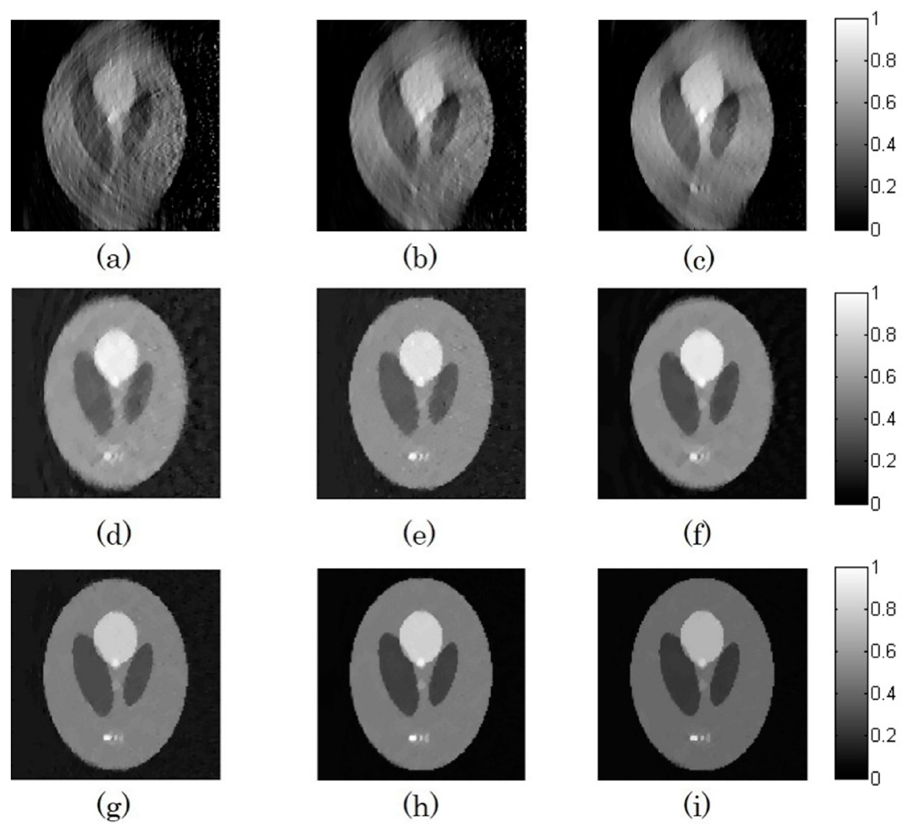
The simulation results are demonstrated in Figure 8. Results show that the TV-GD has the poor performance for the reconstruction. There exists a great degree of distortion in the top right corner as well as the left bottom of the reconstructed images. It has the large error for the geometrical shape between the original image and the reconstructed images. Especially when the views decrease, the result is getting even worse. You can see that for the 60-views scanning in Figure 8a, there is almost no useful information can be obtained from the image except for large tracts of fuzziness. The performance of the TV-VB is better than that of the TV-GD. However, there are still many artifacts that blur the edges of the image in the missing views especially for the 60-views scanning. Besides, the background noise of the results for the TV-VB is serious which affects the image quality. The reconstruction results of the TV-GPEF are superior to that of other two algorithms. The artifacts in those missing views are well suppressed and the image edge information is preserved relatively intact. Almost no blur appears in the reconstructed images for 120-views and 90-views scanning in Figure 8h,i. The contrasts of the images are high and the images are little affected by the noise.
The PSNRs of these three algorithms are shown in Table 2. The results of PSNR also validate the superiority of the proposed algorithm. On average, the PSNR of the TV-GPEF is higher than that of the TV-VB, by about 9 dB and 12 dB, than that of the TV-GD algorithm.
3.3. Noise Robustness
In practical applications, the detected signals are vulnerable to the interference of thermal noise, which is usually Gaussian. Therefore, it is of great importance to test the noise robustness of the algorithm. White Gaussian noise with different powers is added to the detected signals for the case of 20-points straight-line scanning. Then, three groups of noisy signals are acquired with a signal to noise ratio (SNR) of 10 dB, 5 dB and 0 dB, respectively.
The reconstructed images for the three algorithms from the noise-polluted signals are shown in Figure 9. Results show that the TV-GPEF has stronger noise resistance than the other two algorithms. The images from the noisy signals are very close to those from the noise-free signals. Light absorbers in images are clear and distinguishable. The detailed information is quite consistent with the original image. The background noise is well suppressed and there is no significant effect of the added noise to the reconstructed image. However, for the TV-VB and the TV-GD, the added noise has a great influence on the reconstructed images. For the TV-VB, a certain degree of fuzziness appears which blurs the edges of the optical absorbers and there is a lot of background noise in the reconstructed images. The effects of noise are even worse when the SNR decreases. For the result for 0 dB SNR, serious artifacts fuzz up the reconstructed image, which seriously debases the quality of the image. For the TV-GD, the image is severely affected by the added noise and almost all light absorbers are damaged in the reconstructed results.
The PSNRs of the reconstructed images from the noise-added signals for the three algorithms are displayed in Table 3. From the table we can see that the TV-GPEF algorithm outperforms other two algorithms. The PSNR of the TV-GPEF is about 11 dB higher than that of the TV-VB and about 8 dB higher than that of the TV-GD on average. Therefore, we can get the conclusion that the TV-GPEF has the strongest noise robustness compared to the other two algorithms.
3.4. Convergence Speed
Another important performance index for the iterative reconstruction algorithm is the convergence speed. The convergence of an iterative algorithm represents the speed of the reconstructed image approaching to the original one. In order to study the convergence speed of the algorithm, we define the distance between the reconstructed image and the standard image d as follows:
A smaller d means that the reconstructed image is closer to the original image thus the reconstructed result is more accurate and vice versa.
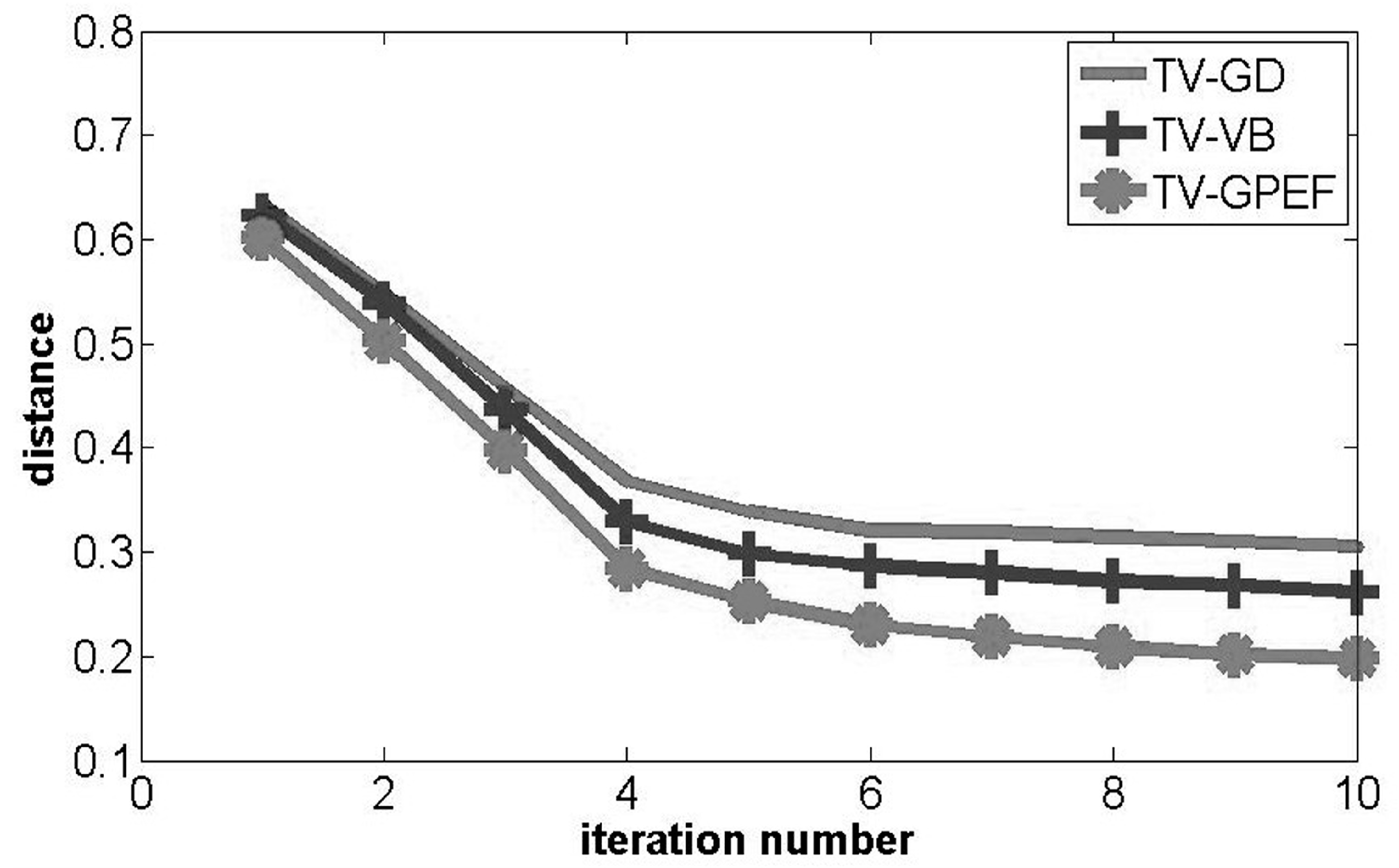
We choose the 90-views limited-angle circular scanning for the study. After each iteration, the obtained reconstructed image is used to calculate the distance d and the calculated d for every step of three algorithms is recorded and compared in a line chart in Figure 10. Results show that the reconstructed image of the TV-GPEF is closer to the real one than other two algorithms for every iteration step. Especially for the first several steps, the d of the TV-GPEF falls even faster than the other two algorithms. After ten iterations, d for three algorithms converges to a certain value and the value of the TV-GPEF is much smaller than those of the two other algorithms. This means that the TV-GPEF is more accurate than other two algorithms. It can be inferred that the proposed TV-GPEF algorithm has faster convergence speed than the other two algorithms.
The computation times for the three algorithms are also compared. The time costs of the three algorithms for 120-views, 90-views, and 60-views limited-angle circular scanning are shown and compared in Table 4. Results show that using variable splitting and Barzilai–Borwein based method to solve the TV-based minimization (TV-VB) can greatly reduce the computation time compared to that of TV-GD. TV-GPEF algorithm has slightly higher computational cost compared to that of the TV-based ones due to the compensation procedure for every iteration. However, the convergence speed for TV-GPEF is greatly improved. In fact, TV-GPEF can obtain better results than that of TV-GD and TV-VB after the same computation time.
From the above discussion, it can be indicated that the TV-GPEF algorithm precedes the other two algorithms in terms of convergence.
4. In Vitro Experiment
In-vitro experiments were also conducted to validate the effectiveness of the proposed TV-GPEF algorithm. Limited-angle circular scanning with 180-views, 90-views and 60-views as well as straight-line scanning were carried out and the reconstructed results for three algorithms were compared and discussed.
The platform for the experiment is shown in Figure 11. The laser we use was a Nd:YAG laser device ( Surelite I, Contimuum, San Jose, CA, USA). The laser pulse with the wavelength of 532 nm was irradiated from the device and reflected by a mirror. Then, it is expanded by a concave mirror and illuminates the object uniformly. The duration of the laser was 4–6 ns and the frequency was 10 Hz. The settings of the laser meeted the American National Standards Institute (ANSI) laser radiation safety standard. The photoacoustic signals were detected by a transducer (V383-SU, Panametrics, Waltham, MA, USA) driven by a stepping motor to scan around the imaged object. The center frequency of the transducer was 3.5 MHz and the bandwidth was 1.12 MHz. The sampling rate of the system was 16.67 MHz.
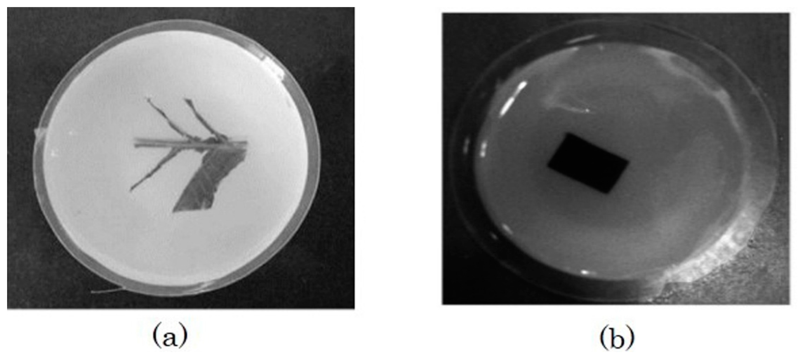
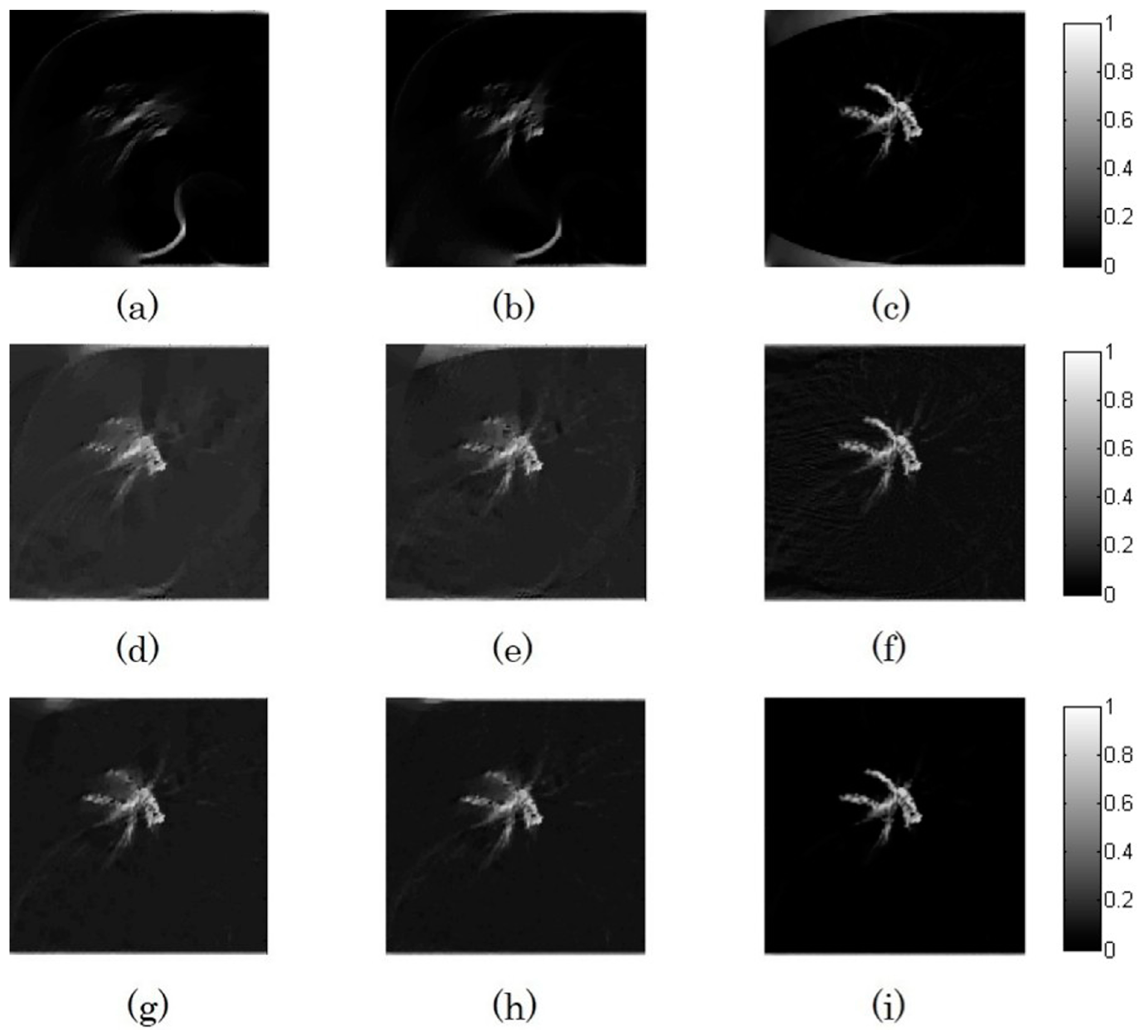
The phantom for the limited-angle circular scanning is shown in Figure 12a. The phantom was made of a gelatin cylinder which had very small light absorption coefficient. The light absorbers were one leaf embedded into the gelatin cylinder. The radius of the phantom was 25 mm. The shape of the phantom imitated the structure of the blood vessel and tissue. The sampling interval was 2°. The 180-views, 90-views and 60-views scanning were conducted, corresponding to the sampling points of 90, 45 and 30, respectively. The scanning radius was 38 mm. The results of the reconstruction for three algorithms are shown in Figure 13. It can be indicated from the results that for the TV-GD, especially when the number of missing views become large, there is serious artifacts and blurs on the reconstructed images. For 90-views and 60-views scanning, almost no useful information for the phantom can be acquired from the results but a blur. For the TV-VB, the performance is improved with respect to the TV-GD. However, there still exist a lot of artifacts in the missing views and edges of the light absorbers are not distinct enough which decreases the resolution of the image. Besides, the background noise also seriously reduces the contrast of the images thus affects the quality of the reconstruction. However for the TV-GPEF, the results are greatly improved. The background noise and the artifacts are suppressed well. The edges of the light absorber are enhanced and the contrast of the image is improved. Therefore, it can be concluded that the performance of the TV-GPEF precedes the two other algorithms in terms of the limited-angle circular scanning.
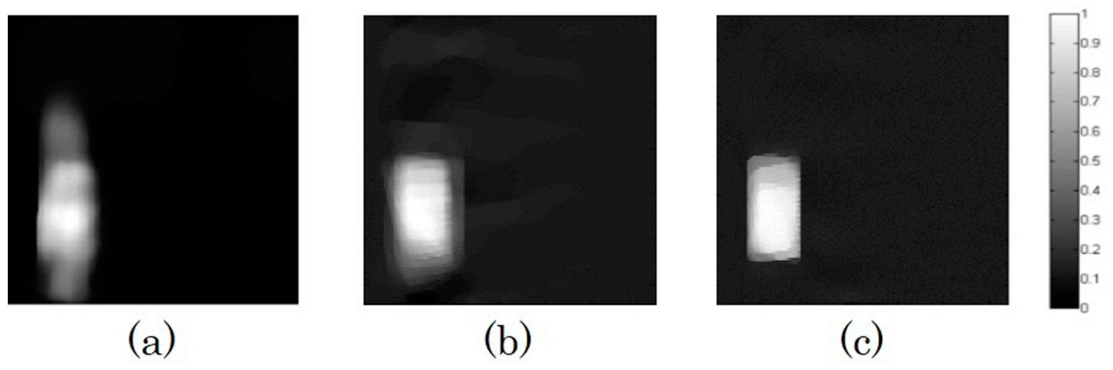
The straight-line scanning was also conducted to verify the proposed algorithm. The phantom for the straight-line scanning is shown in Figure 13b. The phantom was also made of a gelatin cylinder with the radius of 25 mm. A black rectangular rubber sheet was embedded into the gelatin as the light absorber. The size of the rubber sheet was 9 mm × 14 mm. The scanning line was parallel to the longer side of the rectangle. Forty-one sampling points were evenly distributed with the sampling interval of 1 mm. The reconstruction results of three algorithms are demonstrated in Figure 14. For the results of the TV-GD, there is severe deformation for the reconstructed light absorber, especially in the vertical direction. Artifacts with a blade shape appear on the both ends of the light absorber and edges of the image are obscure which are almost hard to recognize. For the TV-VB, the deficiency of the sampling data still causes many artifacts and blurs in the reconstructed image. However, for the TV-GPEF, the missing views are well compensated with fewer artifacts and clearer edges. The distribution of the gray values within the light absorber is relatively uniform. Thus, we can get the conclusion that the TV-GPEF outperforms the other two algorithms in the straight-line scanning.
5. Discussion and Conclusions
In this paper, a Gerchberg–Papoulis extrapolation based compensation method is successfully applied to the limited-view photoacoustic image reconstruction. The missing views are compensated through the extrapolation between the frequency space and image space based on the FFT. This method is more accurate than the iterative-reconstruction-reprojection (IRR) algorithm [40], another transform-based extrapolation method. The IRR algorithm is carried out using the back and forward projection between the image space and projection space. The forward projection usually bases on the relationship in Equation (2), while the back projection on the FBP-based method. This kind of back projection methods, usually solved under a certain ideal condition, requires the completeness of the data. Since the back projection usually does not well match the forward projection, the performance of the IRR method is just average. Therefore, it usually needs interpolations at both the back projection and forward projection stages. The errors for the interpolations would degrade the reconstruction image. Moreover, this mismatched projection pairs also greatly reduce the convergence speed of the algorithm unless sufficient data is available. The FFT-based transformation utilized in the GP-based extrapolation method can effectively improve the accuracy for the compensation without the need for interpolation. Besides, compared to that of the IRR, the adoption of the FFT in the GP-based method can also accelerate the speed for the compensation and then greatly reduce the calculation time. Furthermore, to ensure the convergence of the GP-based algorithm, the known data usually need to be oversampled. To overcome this limitation, the TV-based iteration method is incorporated into the GP-based compensation method and thus greatly improves the convergence speed of the algorithm.
In the GP-based compensation method, the missing detectors are estimated by the reconstructed image acquired from the known data. The image in the missing views is re-estimated by the estimated missing detectors. Then, the compensation is implemented by weightedly adding the estimated image to the former acquired one in the missing views. Adding those two images only in the missing views can avoid the disturbance of the artifacts in the known-region of the estimated image to that of the acquired reconstructed image. The relax factor η can adjust the weight for the estimated image thus can reduce the possibly caused imbalance between the known-views part and missing-views part for the reconstruction results. Thus, before reconstruction, the regions corresponding to the missing views for data and image MS and MI are need to be determined manually based on the scanning pattern. In the future, more effective image infuse methods can be adopted to better integrate those two images instead of just weighted addition so that there is no need to determine MS and MI for each kind of scanning pattern.
λ is the parameter corresponding to the weight of the constraint condition in the optimization problem. Theoretically, the parameter λ does not have a major impact on the performance of the TV-SE algorithm. In addition, the simulations show that the reconstruction results are not sensitive to the value of λ for a large range. Thus, λ is set to a constant 1 in this paper. α is the parameter corresponding to the weight of TV value in the optimization. α with a big value means that the TV-term is dominant which is expected to have a quicker convergence. However, over-sized value will break the balance between the two parts of the objective function. The reconstructed images with over-sized α will have a great difference from the real images because the data fidelity in the reconstruction is sacrificed to image regularity. Based on this criterion, α should be set to a value which is neither too large nor too small compared to the weights of the other part of the objective function. From the simulations and experiments in this manuscript, α can be set from 0.2 to 1. η is a relaxing factor with the range from 0 to 1. It is the weight for the estimated image from GPEF method added to the obtained reconstruction result. Small value of η will diminish the effect of the compensation method while large value of η will affect the accuracy for the results. In addition, from the simulations and experiments, it can be found that when the number of the sampling points or the views for the circular scanning are sufficient, η should be set to a relatively large value to obtain their best performances, whereas, with sparse sampling points or few scanning views, η should be relatively small. From the simulations and experiments, η can be set from 0.05 to 0.3.
In addition, although applying a compensation method to TV-based iterative algorithm will increase the calculation time, the convergence speed of the algorithm is greatly boosted and the quality of the reconstructed images is greatly improved for the limited-view scanning. In addition, the GP-based method using the FFT to estimate the missing views between the image space and frequency space can accelerate the algorithm and ensure its accuracy. Besides, the adoption of the effective variable splitting and Barzilai–Borwein based method to solve the optimization problem can also increase the convergence speed while reducing the calculation time of the algorithm. Moreover, the experimental design in this paper is relatively simple and is constrained by the equipment of the experiment such as the low-frequency transducer. Future work will focus on the improvement of the experimental facilities and will try more complicated experiments on animals.
Finally, the proposed TV-GPEF algorithm is verified by both numerical simulations and in vitro experiments. The different views of limited-angle circular scanning and straight-line scanning with varying sampling points are conducted. The reconstructed results of the proposed algorithm are compared to those of the TV-GD and TV-VB algorithm. Results show that the TV-GPEF is superior to the other two algorithms and it will greatly improve the performance for the limited-view scanning. The artifacts caused by the missing views are well compensated and the distortion and blurring for the image are greatly reduced. Thus, edges of the image are enhanced and details of the information are better preserved. For the limited-angle circular scanning, the PSNR of the TV-GPEF is higher than that of the TV-GD for about 11 dB and that of the TV-VB for 7 dB on average. For the straight-line scanning, the amplification is 12 dB to the TV-GD and 9 dB to the TV-VB. Besides, the proposed TV-GPEF algorithm also precedes the two other algorithms in terms of noise robustness and convergence speed. Consequently, we can conclude that the proposed TV-GPEF algorithm is applicable to limited-view PAI and can well solve the problem of the incompleteness of the sampling data.
Acknowledgments
This work was supported by the National Basic Research Program of China (2015CB755500) the National Natural Science Foundation of China (No. 11474071).
Author Contributions
Study concept and design: Jin Wang; drafting of the manuscript: Jin Wang; critical revision of the manuscript for important intellectual content: Jin Wang and Yuanyuan Wang; obtained funding: Yuanyuan Wang; administrative, technical, and material support: Jin Wang and Yuanyuan Wang; and study supervision: Yuanyuan Wang. All authors read and approved the final manuscript.
Conflicts of Interest
The authors declare no conflict of interest.
References
- Li, C.; Wang, L.V. Photoacoustic tomography and sensing in biomedicine. Phys. Med. Biol. 2009, 54, R59–R97. [Google Scholar] [CrossRef] [PubMed]
- Wang, L.V. Prospects of photoacoustic tomography. Med. Phys. 2008, 35, 5758–5767. [Google Scholar] [CrossRef] [PubMed]
- Xu, M.; Wang, L.V. Photoacoustic imaging in biomedicine. Rev. Sci. Instrum. 2006, 77, 041101. [Google Scholar] [CrossRef]
- Kim, C.; Favazza, C.; Wang, L.V. In vivo photoacoustic tomography of chemicals: High-resolution functional and molecular optical imaging at new depths. Chem. Rev. 2010, 110, 2756–2782. [Google Scholar] [CrossRef] [PubMed]
- Li, J.; Xiao, H.; Yoon, S.J.; Liu, C.; Matsuura, D.; Tai, W.; Song, L.; O’Donnell, M.; Cheng, D.; Gao, X. Functional photoacoustic imaging of gastric acid secretion using pH-responsive polyaniline nanoprobes. Small 2016, 12, 4690–4696. [Google Scholar] [CrossRef] [PubMed]
- Stein, E.W.; Maslov, K.; Wang, L.V. Noninvasive, in vivo imaging of blood-oxygenation dynamics within the mouse brain using photoacoustic microscopy. J. Biomed. Opt. 2009, 14, 020502. [Google Scholar] [CrossRef] [PubMed]
- Wang, D.; Wu, Y.; Xia, J. Review on photoacoustic imaging of the brain using nanoprobes. Neurophotonics 2016, 3, 010901. [Google Scholar] [CrossRef] [PubMed]
- Yang, X.; Wang, L.V. Monkey brain cortex imaging by photoacoustic tomography. J. Biomed. Opt. 2008, 13, 044009. [Google Scholar] [CrossRef] [PubMed]
- Lu, J.; Gao, Y.; Ma, Z.; Zhou, H.; Wang, R.K.; Wang, Y. In vivo photoacoustic imaging of blood vessels using a homodyne interferometer with zero-crossing triggering. J. Biomed. Opt. 2017, 22, 036002. [Google Scholar] [CrossRef] [PubMed]
- Zhong, J.; Wen, L.; Yang, S.; Xiang, L.; Chen, Q.; Xing, D. Imaging-guided high-efficient photoacoustic tumor therapy with targeting gold nanorods. Nanomed. Nanotechnol. Biol. Med. 2015, 11, 1499–1509. [Google Scholar] [CrossRef] [PubMed]
- Pu, K.; Shuhendler, A.J.; Jokerst, J.V.; Mei, J.; Gambhir, S.S.; Bao, Z.; Rao, J. Semiconducting polymer nanoparticles as photoacoustic molecular imaging probes in living mice. Nat. Nanotechnol. 2014, 9, 233–239. [Google Scholar] [CrossRef] [PubMed]
- Jose, J.; Willemink, R.G.; Resink, S.; Piras, D.; van Hespen, J.G.; Slump, C.H.; Steenbergen, W.; van Leeuwen, T.G.; Manohar, S. Passive element enriched photoacoustic computed tomography (PER PACT) for simultaneous imaging of acoustic propagation properties and light absorption. Opt. Express 2011, 19, 2093–2104. [Google Scholar] [CrossRef] [PubMed]
- Yao, J.; Xia, J.; Maslov, K.I.; Nasiriavanaki, M.; Tsytsarev, V.; Demchenko, A.V.; Wang, L.V. Noninvasive photoacoustic computed tomography of mouse brain metabolism in vivo. Neuroimage 2013, 64, 257–266. [Google Scholar] [CrossRef] [PubMed]
- Strohm, E.M.; Moore, M.J.; Kolios, M.C. Single cell photoacoustic microscopy: A review. IEEE J. Sel. Top. Quantum Electron. 2016, 22, 137–151. [Google Scholar] [CrossRef]
- Zhang, C.; Maslov, K.; Wang, L.V. Subwavelength-resolution label-free photoacoustic microscopy of optical absorption in vivo. Opt. Lett. 2010, 35, 3195–3197. [Google Scholar] [CrossRef] [PubMed]
- Kruger, R.A.; Liu, P.; Fang, Y.; Appledorn, C.R. Photoacoustic ultrasound (PAUS)—Reconstruction tomography. Med. Phys. 1995, 22, 1605–1609. [Google Scholar] [CrossRef] [PubMed]
- Mohajerani, P.; Kellnberger, S.; Ntziachristos, V. Fast Fourier backprojection for frequency-domain optoacoustic tomography. Opt. Lett. 2014, 39, 5455–5458. [Google Scholar] [CrossRef] [PubMed]
- Xu, M.; Xu, Y.; Wang, L.V. Time-domain reconstruction algorithms and numerical simulations for thermoacoustic tomography in various geometries. IEEE Trans. Biomed. Eng. 2003, 50, 1086–1099. [Google Scholar] [CrossRef] [PubMed]
- Xu, Y.; Feng, D.; Wang, L.V. Exact frequency-domain reconstruction for thermoacoustic tomography. I. Planar geometry. IEEE Trans. Med. Imaging 2002, 21, 823–828. [Google Scholar] [CrossRef] [PubMed]
- Zhang, C.; Wang, Y. Deconvolution reconstruction of full-view and limited-view photoacoustic tomography: A simulation study. J. Opt. Soc. Am. 2008, 25, 2436–2443. [Google Scholar] [CrossRef]
- Finch, D.; Patch, S.K. Determining a function from its mean values over a family of spheres. SIAM J. Math. Anal. 2004, 35, 1213–1240. [Google Scholar] [CrossRef]
- Finch, D.; Haltmeier, M.; Rakesh. Inversion of spherical means and the wave equation in even dimensions. SIAM J. Appl. Math. 2007, 68, 392–412. [Google Scholar] [CrossRef]
- Kunyansky, L.A. Explicit inversion formulae for the spherical mean Radon transform. Inverse Probl. 2007, 23, 373–383. [Google Scholar] [CrossRef]
- Haltmeier, M. Universal inversion formulas for recovering a function from spherical means. SIAM J. Math. Anal. 2014, 46, 214–232. [Google Scholar] [CrossRef]
- Huang, C.; Wang, K.; Nie, L.; Wang, L.V.; Anastasio, M.A. Full-wave iterative image reconstruction in photoacoustic tomography with acoustically inhomogeneous media. IEEE Trans. Med. Imaging 2013, 32, 1097–1110. [Google Scholar] [CrossRef] [PubMed]
- Paltauf, G.; Viator, J.; Prahl, S.; Jacques, S. Iterative reconstruction algorithm for optoacoustic imaging. J. Acoust. Soc. Am. 2002, 112, 1536–1544. [Google Scholar] [CrossRef] [PubMed]
- Rosenthal, A.; Jetzfellner, T.; Razansky, D.; Ntziachristos, V. Efficient framework for model-based tomographic image reconstruction using wavelet packets. IEEE Trans. Med. Imaging 2012, 31, 1346–1357. [Google Scholar] [CrossRef] [PubMed]
- Ding, L.; Deán-Ben, X.L.; Lutzweiler, C.; Razansky, D.; Ntziachristos, V. Efficient non-negative constrained model-based inversion in optoacoustic tomography. Phys. Med. Biol. 2015, 60, 6733–6750. [Google Scholar] [CrossRef] [PubMed]
- Meng, J.; Wang, L.V.; Ying, L.; Liang, D.; Song, L. Compressed-sensing photoacoustic computed tomography in vivo with partially known support. Opt. Express 2012, 20, 16510–16523. [Google Scholar] [CrossRef] [PubMed]
- Haltmeier, M.; Berer, T.; Moon, S.; Burgholzer, P. Compressed sensing and sparsity in photoacoustic tomography. J. Opt. 2016, 18, 114004. [Google Scholar] [CrossRef]
- Betcke, M.M.; Cox, B.T.; Huynh, N.; Zhang, E.Z.; Beard, P.C.; Arridge, S.R. Acoustic wave field reconstruction from compressed measurements with application in photoacoustic tomography. arXiv, 2016; arXiv:1609.02763. [Google Scholar]
- Arridge, S.; Beard, P.; Betcke, M.; Cox, B.; Huynh, N.; Lucka, F.; Ogunlade, O.; Zhang, E. Accelerated high-resolution photoacoustic tomography via compressed sensing. Phys. Med. Biol. 2016, 61, 8908–8940. [Google Scholar] [CrossRef] [PubMed]
- Wang, K.; Su, R.; Oraevsky, A.A.; Anastasio, M.A. Investigation of iterative image reconstruction in three-dimensional optoacoustic tomography. Phys. Med. Biol. 2012, 57, 5399–5423. [Google Scholar] [CrossRef] [PubMed]
- Zhang, Y.; Wang, Y.; Zhang, C. Total variation based gradient descent algorithm for sparse-view photoacoustic image reconstruction. Ultrasonics 2012, 52, 1046–1055. [Google Scholar] [CrossRef] [PubMed]
- Gamelin, J.K.; Aguirre, A.; Zhu, Q. Fast, limited-data photoacoustic imaging for multiplexed systems using a frequency-domain estimation technique. Med. Phys. 2011, 38, 1503–1518. [Google Scholar] [CrossRef] [PubMed]
- Wu, D.; Tao, C.; Liu, X. Photoacoustic tomography in scattering biological tissue by using virtual time reversal mirror. J. Appl. Phys. 2011, 109, 084702. [Google Scholar] [CrossRef]
- Yao, L.; Jiang, H. Photoacoustic image reconstruction from few-detector and limited-angle data. Biomed. Opt. Express 2011, 2, 2649–2654. [Google Scholar] [CrossRef] [PubMed]
- Xu, Y.; Wang, L.V.; Ambartsoumian, G.; Kuchment, P. Reconstructions in limited-view thermoacoustic tomography. Med. Phys. 2004, 31, 724–733. [Google Scholar] [CrossRef] [PubMed]
- Xiang, L.Z.; Xing, D.; Gu, H.M.; Yang, S.H.; Zeng, L.M. Photoacoustic imaging of blood vessels based on modified simultaneous iterative reconstruction technique. Acta Phys. Sin. 2007, 56, 3911–3916. [Google Scholar]
- Tao, C.; Liu, X. Reconstruction of high quality photoacoustic tomography with a limited-view scanning. Opt. Express 2010, 18, 2760–2766. [Google Scholar] [CrossRef] [PubMed]
- Zhang, C.; Zhang, Y.; Wang, Y. A photoacoustic image reconstruction method using total variation and nonconvex optimization. Biomed. Eng. Online 2014, 13, 117. [Google Scholar] [CrossRef] [PubMed]
- Liu, X.; Peng, D.; Ma, X.; Guo, W.; Liu, Z.; Han, D.; Yang, X.; Tian, J. Limited-view photoacoustic imaging based on an iterative adaptive weighted filtered backprojection approach. Appl. Opt. 2013, 52, 3477–3483. [Google Scholar] [CrossRef] [PubMed]
- Modgil, D.; La, P.J. Riviere, Implementation and comparision of reconstruction algorithms for 2D optoacoustic tomography using a linear array. Proc. SPIE 2008, 6856, 68561D-1–68561D-12. [Google Scholar] [CrossRef]
- Gao, H.; Feng, J.; Song, L. Limited-view multi-source quantitative photoacoustic tomography. Inverse Probl. 2015, 31, 065004. [Google Scholar] [CrossRef]
- Huang, B.; Xia, J.; Maslov, K.; Wang, L.V. Improving limited-view photoacoustic tomography with an acoustic reflector. J. Biomed. Opt. 2013, 18, 110505. [Google Scholar] [CrossRef] [PubMed]
- Feng, J.; Zhou, W.; Gao, H. Multi-source Quantitative Photoacoustic Tomography with Detector Response Function and Limited-view Scanning. J. Comput. Math. 2016, 34, 588–607. [Google Scholar] [CrossRef]
- Gerchberg, R. Super-resolution through error energy reduction. J. Mod. Opt. 1974, 21, 709–720. [Google Scholar] [CrossRef]
- Papoulis, A. A new algorithm in spectral analysis and band-limited extrapolation. IEEE Trans. Circuits Syst. 1975, 22, 735–742. [Google Scholar] [CrossRef]
- Rudin, L.I.; Osher, S.; Fatemi, E. Nonlinear total variation based noise removal algorithms. Physica D 1992, 60, 259–268. [Google Scholar] [CrossRef]
- Gao, H.; Zhang, L.; Chen, Z.; Xing, Y.; Xue, H.; Cheng, J. Straight-line-trajectory-based x-ray tomographic imaging for security inspections: system design, image reconstruction and preliminary results. IEEE Trans. Nucl. Sci. 2013, 60, 3955–3968. [Google Scholar] [CrossRef]
- Köstli, K.P.; Beard, P.C. Two-dimensional photoacoustic imaging by use of Fourier-transform image reconstruction and a detector with an anisotropic response. Appl. Opt. 2003, 42, 1899–1908. [Google Scholar] [CrossRef] [PubMed]
- Ye, X.; Chen, Y.; Huang, F. Computational acceleration for MR image reconstruction in partially parallel imaging. IEEE Trans. Med. Imaging 2011, 30, 1055–1063. [Google Scholar] [CrossRef] [PubMed]
- Afonso, M.V.; Bioucas-Dias, J.M.; Figueiredo, M.A. An augmented Lagrangian approach to the constrained optimization formulation of imaging inverse problems. IEEE Trans. Image Process. 2011, 20, 681–695. [Google Scholar] [CrossRef] [PubMed]
Figure 1.
The diagram of the Gerchberg-Papoulis-based compensation method. The dots in the left and right subfigures refer to the positions of the known detectors (left) and the estimated detectors (right).
Figure 1.
The diagram of the Gerchberg-Papoulis-based compensation method. The dots in the left and right subfigures refer to the positions of the known detectors (left) and the estimated detectors (right).

Figure 2.
The Sheep–Logan phantom and the diagram for the straight-line scanning.
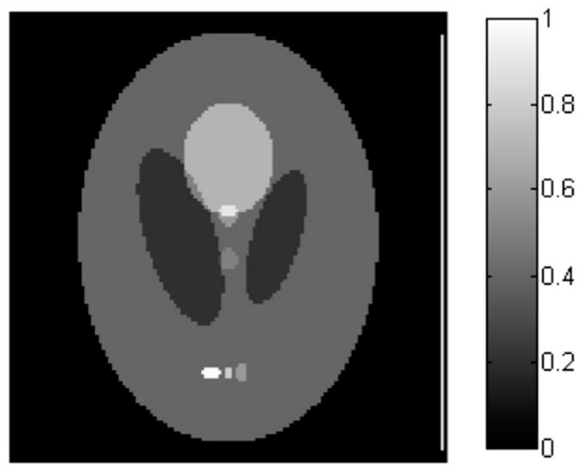
Figure 3.
The position of the estimated detectors (dots “·”) and the corresponding image region to the missing views which needs compensation (white area in the image). The position of the measured detectors (dots “*”) and the corresponding known area of the image (black area in the image).
Figure 3.
The position of the estimated detectors (dots “·”) and the corresponding image region to the missing views which needs compensation (white area in the image). The position of the measured detectors (dots “*”) and the corresponding known area of the image (black area in the image).
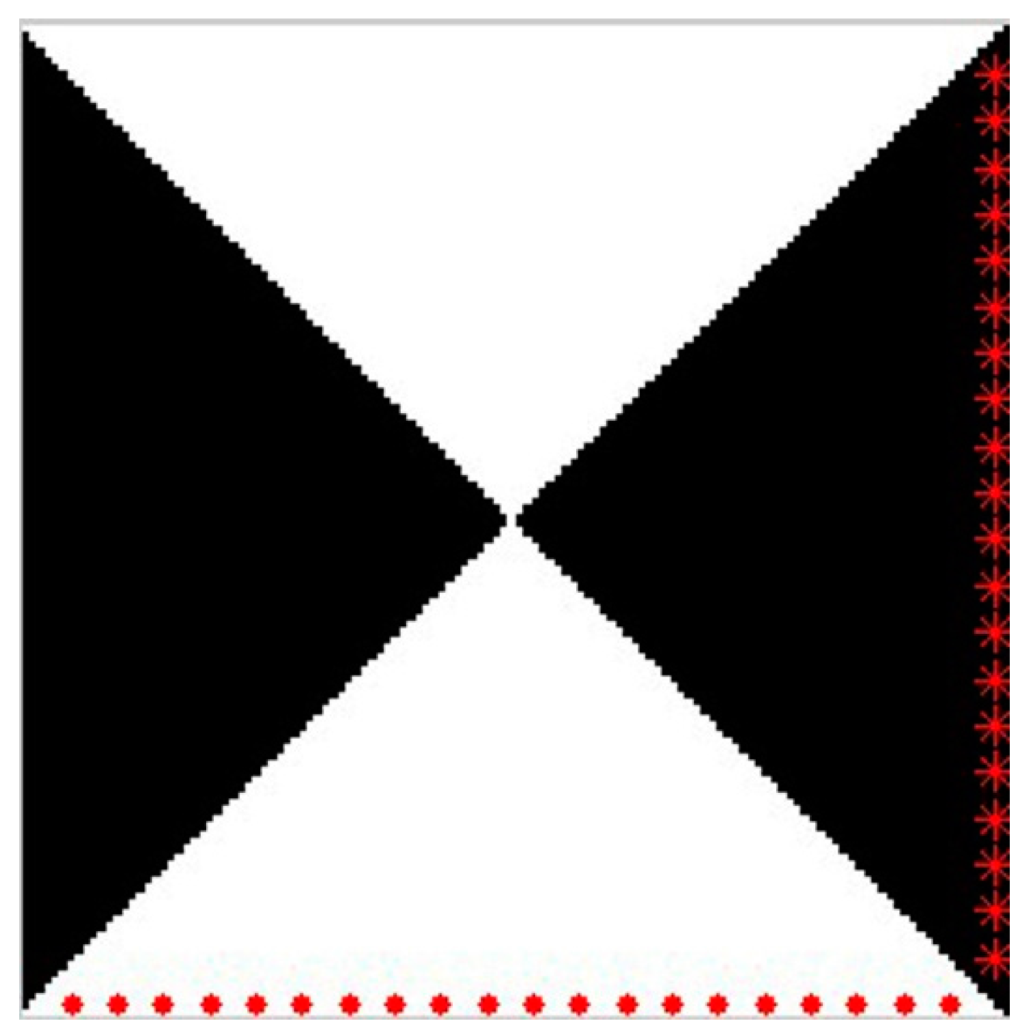
Figure 4.
The reconstructed images from the straight-line scanning by the TV-GD (TV-based algorithm solved by gradient descent method), TV-VB (TV-based algorithm solved by the variable splitting and Barzilai–Borwein based method) and TV-GPEF (TV-based algorithm incorporated with Gerchberg-Papoulis-based FFT-utilized compensation method) algorithms: the first row refers to the results of the TV-GD (a–c); the second row refers to the results of the TV-VB (d–f); and the third row refers to the results of the TV-GPEF (g–i). The first to third columns refer to the results from: 50-points (a,d,g); 20-points (b,e,h); and 10-points (c,f,i) sampling, respectively.
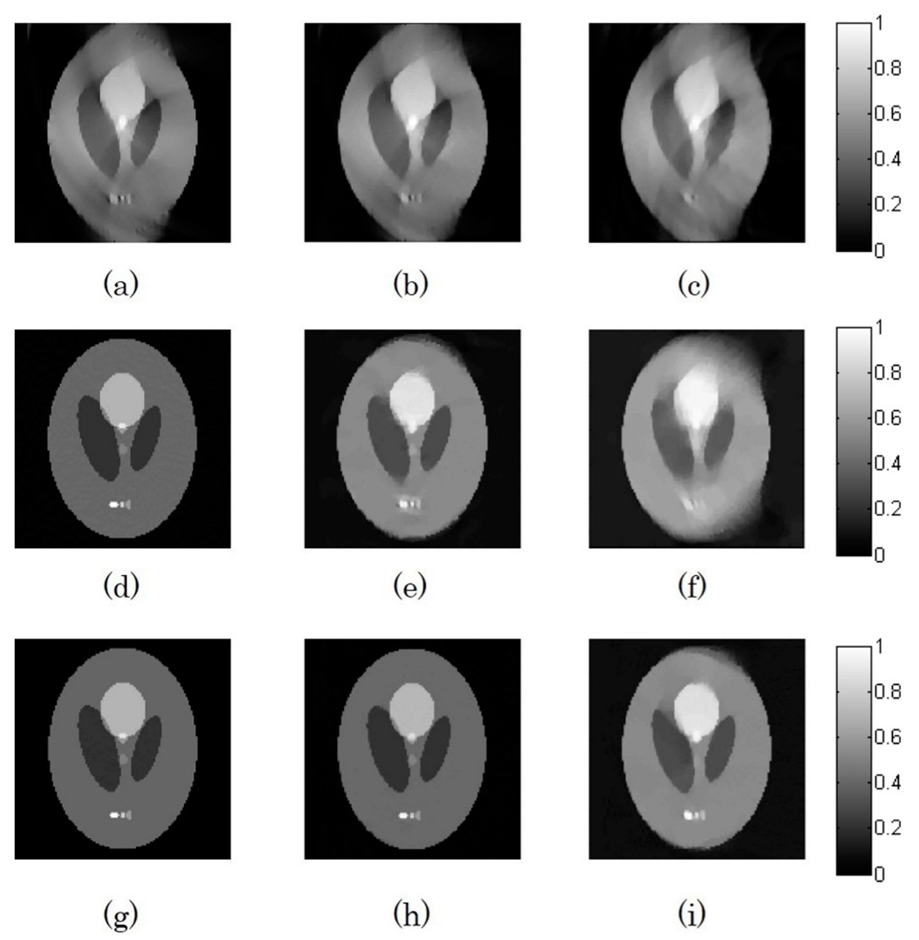
Figure 5.
The line chart of the Peak signal-to-noise rations (PSNRs) (dB) versus the number of estimated detectors for the straight-line scanning for TV-GPEF.
Figure 5.
The line chart of the Peak signal-to-noise rations (PSNRs) (dB) versus the number of estimated detectors for the straight-line scanning for TV-GPEF.

Figure 6.
The diagram for the limited-angle circular scanning with: 60-views (a); 90-views (b); and 120-views (c).
Figure 6.
The diagram for the limited-angle circular scanning with: 60-views (a); 90-views (b); and 120-views (c).
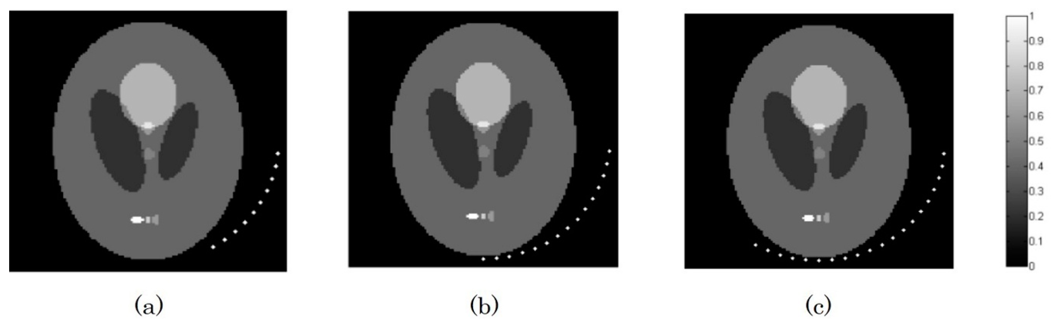
Figure 7.
The position of the estimated detectors (dots “·”) and the corresponding image region to the missing detectors which needs compensation (white area in the image). The position of the measured detectors (dots “*”) and the corresponding known area of the image (black area in the image). Panels (a–c) refer to 60-views, 90-views and 120-views circular scanning, respectively.
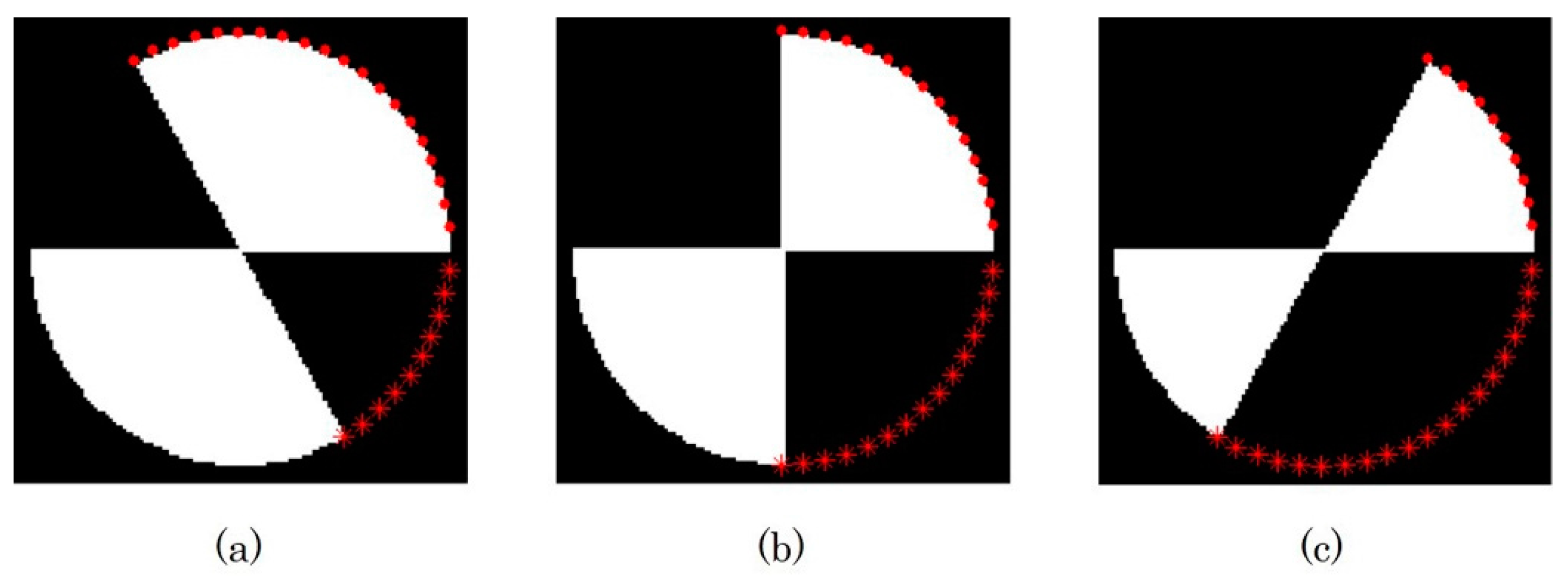
Figure 8.
The reconstructed images from the limited-angle circular scanning by the TV-GD, TV-VB and TV-GPEF algorithms: the first row refers to the results of the TV-GD (a–c); the second row refers to the results of the TV-VB (d–f); and the third row refers to the results of the TV-GPEF (g–i). The first to third columns refer to the results from: 60-views (a,d,g); 90-views (b,e,h); and 120-views (c,f,i) sampling, respectively.

Figure 9.
The reconstructed images from the noise-added signals by the TV-GD, TV-VB and TV-GPEF algorithms: the first row refers to the results of the TV-GD (a–c); the second row refers to the results of the TV-VB (d–f); and the third row refers to the results of the TV-GPEF (g–i). The first to third columns refer to the results from SNR of: 10 dB (a,d,g); 5 dB (b,e,h); and 0 dB (c,f,i) sampling, respectively.

Figure 10.
The line chart of the distance between the reconstructed image and the original image for each iteration from the TV-GD, TV-VB and TV-GPEF algorithms.
Figure 10.
The line chart of the distance between the reconstructed image and the original image for each iteration from the TV-GD, TV-VB and TV-GPEF algorithms.

Figure 11.
Scheme of the platform used for the experiments.
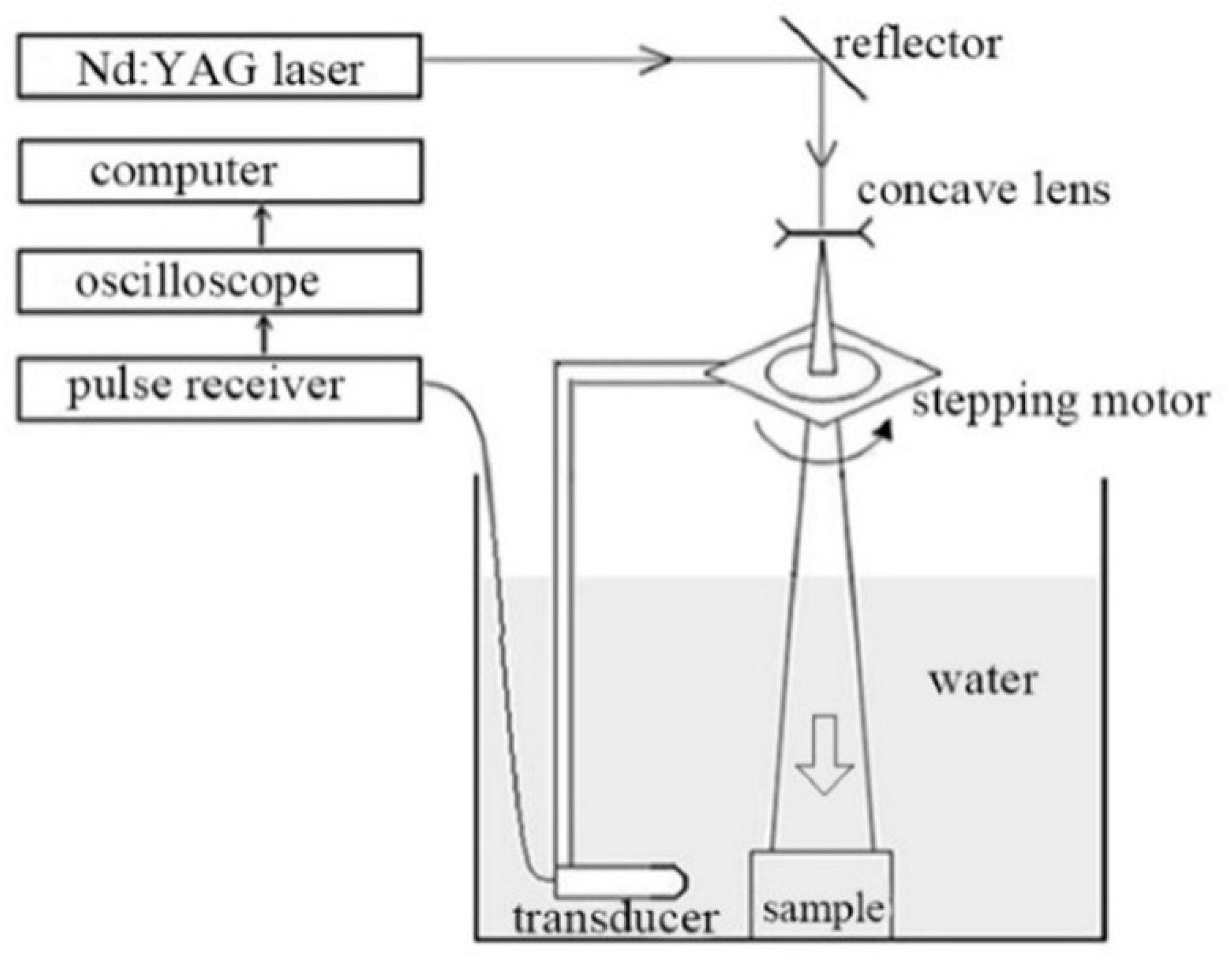
Figure 12.
Pictures of the phantoms used in the experiments: (a) for the limited-angle circular scanning; and (b) for the straight-line scanning.
Figure 12.
Pictures of the phantoms used in the experiments: (a) for the limited-angle circular scanning; and (b) for the straight-line scanning.

Figure 13.
The reconstructed images from the phantom in Figure 10 by the TV-GD, TV-VB and TV-GPEF algorithms-: the first row refers to the results of the TV-GD (a–c); the second row refers to the results of the TV-VB (d–f); and the third row refers to the results of the TV-GPEF (g–i). The first to third columns refer to the results from the limited-angle circular scanning of: 60-views (a,d,g); 90-views (b,e,h); and 180-views (c,f,i) sampling, respectively.

Figure 14.
The reconstructed images from the phantom in Figure 10b: (a) TV-GD; (b) TV-VB; and (c) TV-GPEF algorithms for the straight-line scanning.
Figure 14.
The reconstructed images from the phantom in Figure 10b: (a) TV-GD; (b) TV-VB; and (c) TV-GPEF algorithms for the straight-line scanning.

Table 1.
Peak signal-to-noise rations (PSNRs) (dB) of the straight-line scanning from the Sheep-Logan phantom.
Table 1.
Peak signal-to-noise rations (PSNRs) (dB) of the straight-line scanning from the Sheep-Logan phantom.
| PSNRs (dB) | 50-Points | 20-Points | 10-Points |
|---|---|---|---|
| TV-GD | 17.58 | 16.46 | 14.35 |
| TV-VB | 26.58 | 19.34 | 15.26 |
| TV-GPEF | 32.56 | 28.67 | 22.23 |
Table 2.
PSNR (dB) of the limited-angle circular scanning from the Sheep–Logan phantom.
| PSNRs (dB) | 60-Views | 90-Views | 120-Views |
|---|---|---|---|
| TV-GD | 12.23 | 14.49 | 18.78 |
| TV-VB | 14.41 | 18.03 | 22.47 |
| TV-GPEF | 21.89 | 26.71 | 33.74 |
Table 3.
PSNR (dB) of the reconstruction from the noise-added signals.
| PSNRs (dB) | 0 dB | 5 dB | 10 dB |
|---|---|---|---|
| TV-GD | 12.59 | 13.47 | 14.02 |
| TV-VB | 14.97 | 16.49 | 18.55 |
| TV-GPEF | 21.38 | 25.32 | 27.39 |
Table 4.
Computation cost for the reconstruction from limited-angle circular scanning.
| Time (s) | 180-Views | 90-Views | 60-Views |
|---|---|---|---|
| TV-GD | 15.68 | 13.73 | 10.32 |
| TV-VB | 9.87 | 8.37 | 6.14 |
| TV-GPEF | 16.43 | 14.46 | 11.28 |
© 2017 by the authors. Licensee MDPI, Basel, Switzerland. This article is an open access article distributed under the terms and conditions of the Creative Commons Attribution (CC BY) license (http://creativecommons.org/licenses/by/4.0/).
Share and Cite
MDPI and ACS Style
Wang, J.; Wang, Y. An Efficient Compensation Method for Limited-View Photoacoustic Imaging Reconstruction Based on Gerchberg–Papoulis Extrapolation. Appl. Sci. 2017, 7, 505. https://doi.org/10.3390/app7050505
AMA Style
Wang J, Wang Y. An Efficient Compensation Method for Limited-View Photoacoustic Imaging Reconstruction Based on Gerchberg–Papoulis Extrapolation. Applied Sciences. 2017; 7(5):505. https://doi.org/10.3390/app7050505
Chicago/Turabian StyleWang, Jin, and Yuanyuan Wang. 2017. "An Efficient Compensation Method for Limited-View Photoacoustic Imaging Reconstruction Based on Gerchberg–Papoulis Extrapolation" Applied Sciences 7, no. 5: 505. https://doi.org/10.3390/app7050505
Note that from the first issue of 2016, this journal uses article numbers instead of page numbers. See further details here.