
Stochastic Model Predictive Control for Urban Traffic Networks

1
College of Mechanical and Electrical Engineering, Jiaxing University, Jiaxing 314001, China
2
Institute of Cyber-Systems and Control, College of Control Science and Engineering, Zhejiang University, Hangzhou 310024, China
3
College of Biological, Chemical Sciences and Engineering, Jiaxing University, Jiaxing 314001, China
*
Author to whom correspondence should be addressed.
Appl. Sci. 2017, 7(6), 588; https://doi.org/10.3390/app7060588
Submission received: 13 April 2017
/
Revised: 19 May 2017
/
Accepted: 2 June 2017
/
Published: 7 June 2017
Abstract
:This paper proposes a stochastic model predictive control (MPC) framework for traffic signal coordination and control in urban traffic networks. One of the important features of the proposed stochastic MPC model is that uncertain traffic demands and stochastic disturbances are taken into account. Aiming to effectively model the uncertainties and avoid queue spillback in traffic networks, we develop a stochastic expected value model with chance constraints for the objective function of the stochastic MPC model. The objective function is defined to minimize the queue length and the oscillation of green time between any two control steps. Furthermore, by embedding the stochastic simulation and neural networks into a genetic algorithm, we propose a hybrid intelligent algorithm to solve the stochastic MPC model. Finally, numerical results by means of simulation on a road network are presented, which illustrate the performance of the proposed approach.
1. Introduction
In many major metropolitan areas, inevitable delays and traffic congestion would be incurred by road users due to inappropriate design of traffic signal settings and uncertain traffic demand in road networks. Therefore, developing effective traffic signal control strategies for urban road networks has long been one of the imperative issues for traffic researchers and practitioners. In general, traffic signal control methodologies can be classified into three categories (Isolated Intersection Control, Fixed Time Coordinated Control and Coordinated Traffic-Responsive Control) by their characteristics [1].
As one of the earliest and simplest methods, isolated intersection control strategy is mainly used to access the optimal signal timing plan of an isolated intersection. Therefore, in many cases, it is a myopic control approach [2,3]. Since their settings are based on history traffic flow information, fixed time coordinated control strategies can only provide good control performance under the condition of minor fluctuations in traffic demand [4]. As a result, coordinated traffic-responsive control strategies are proposed to overcome the drawbacks that existed in the previous two methods. Since the 1970s, lots of model-based traffic-responsive control strategies have been proposed. For example, SCOOT [5], SCATS [6], OPAC [7], PRODYN [8], and RHODES [9] are widely used in many cities. It is worth mentioning that the store-and-forward(SF) approach [10] is also one of the typical representatives in the family of coordinated traffic-responsive control strategies. Based on the SF approach, a number of traffic models and control strategies [11,12,13,14] have been proposed.
Without a doubt, a suitable traffic model can not only be convenient to assist traffic engineers to analyze the traffic dynamics, but also provides the basis for designing effective traffic signal control strategies. Since model predictive control (MPC) can deal with complex constraints and avoid myopic control schemes in large-scale control problems, MPC approaches are used to model and coordinate traffic signals in urban traffic networks [15,16,17,18,19,20,21,22]. For instance, the authors in [15] proposed a linear model and a multi-agent control strategy for traffic signal coordination in urban traffic networks (UTN). In their model, by decomposing the centralized MPC problem into a number of coupled subproblems, the original control problem was solved by several distributed agents. Based on this work, a distributed interior-point algorithm was proposed to speed up the solving process in [16]. By using an improved nonlinear traffic flow model, Ref. [17] proposed a centralized MPC model for network-wide traffic signal coordination. In addition, the optimization model reported in [17] was improved and replaced by a mixed-integer linear programming model in [18]. To enhance the computational efficiency and make the application of the MPC approach feasible for large scale urban traffic networks, hierarchical (or decentralized) and distributed MPC models can be found in later works [19,20,21,22].
It is worth noting that the MPC methods aforementioned are all designed within a deterministic framework. However, uncertainties widely exist in reality and urban traffic networks are no exception. Hence, uncertainties (e.g., uncertain traffic demand, stochastic disturbances) have to be investigated in traffic model building. It is well known that using appropriate tools or methods to deal with uncertainties in traffic networks is very important for accessing the optimal signal timing plan of traffic networks. To our knowledge, so far, the studies that take these uncertainties into consideration on modeling of traffic signal control are rarely seen particularly under MPC framework. Aiming to minimize the average delays under changing traffic demand, Ref. [23] proposed three models to determine optimal signal timing plan. Ref. [24] reported a stochastic optimization method to access a robust signal timing plan for arterial signal coordination, in which day-to-day demand variations were taken into account. Ref. [25] proposed a robust MPC model and a constrained mini-max approach to achieve optimal signal splits for urban traffic networks, in which uncertainties (e.g., inaccurate nominal state and demand prediction) were taken into account and assumed to be bounded. However, in their work, the objective function was defined to access the minimal cost under the largest possible model uncertainties. Accordingly, the optimal solution reported in [25] was calculated from a worst-case scenario formulation. Ref. [26] proposed a receding horizon parameterized control method for freeway networks. In this method, a scenario-based min-max scheme is designed to handle uncertainties. The authors in [27] proposed a novel MPC model for traffic signal control, whereby chance constraints are embedded into the model to prevent the arteries in the traffic network over-saturated in stressed load situations. Nevertheless, the uncertain model reported in [27] mainly focuses on preventing queue spillback on major trunk roads.
Different from the aforementioned studies, by utilizing the store-and-forward model, we propose a stochastic MPC framework for traffic signal coordination in urban traffic networks. The objectives of the proposed stochastic MPC model are to prevent queue spill-back and to shorten the queue length of the whole network. One of the important features of our framework is that chance constrained programming [28] is used to handle uncertain traffic demands and stochastic disturbances on traffic networks. Furthermore, by embedding the stochastic simulation and neural networks (NNs) [29,30] into a genetic algorithm (GA) [28,31], we propose a hybrid intelligent approach to solve the uncertain optimization problem of the traffic network.
The outline of this paper is organized as follows. In Section 2, we employ an improved store-and-forward traffic model to describe the traffic dynamics in urban traffic networks (UTN). In Section 3, a stochastic MPC model for UTN is proposed. In the proposed stochastic MPC model, uncertain traffic demands and disturbances are both taken into account and modeled by chance constrained programming. To avoid the spill-back congestion and reduce the queue length, chance constraints are imposed on the queue length of the road network. In Section 4, we propose a hybrid intelligent method to solve the stochastic MPC model. Section 5 reports the results of numerical simulation which aimed to verify the effectiveness of the proposed model and solution method. Finally, Section 6 concludes this paper with a summary of work.
2. Modeling of Traffic Dynamics
2.1. Notations
An overview of the notations used in this paper is presented below. We define the discrete time step as k, the prediction horizon length as P, the sampling time as T, the number of vehicles within link r of intersection i at the beginning of the kth time interval as , the effective green time of phase p of intersection i as and the set of phases of intersection i as . The lost time and cycle time of each intersection i satisfy . In addition, the saturation flow of each link is defined as . Let denote the turning rate. It means that the rate of vehicles that reach the link r of intersection i from the link w of intersection j is .
2.2. Traffic Dynamics
To optimize traffic signal splits, Gazis and Potts proposed a Store-and-forward (SF) method [10] in 1963. In the SF method, they designed a simplified linear model to describe traffic dynamics in UTN. Since the linear model allows the use of high efficient control and optimization technology for signal coordination in large-scale networks, the SF method has been widely used for modeling and optimization of traffic signal splits in road networks [11,12,13,14,15,16,19,20]. Therefore, in this paper, we use an improved SF method [20,22] to model the traffic dynamics. The technique defines a simple vehicle-conservation equation between two signalized intersections.
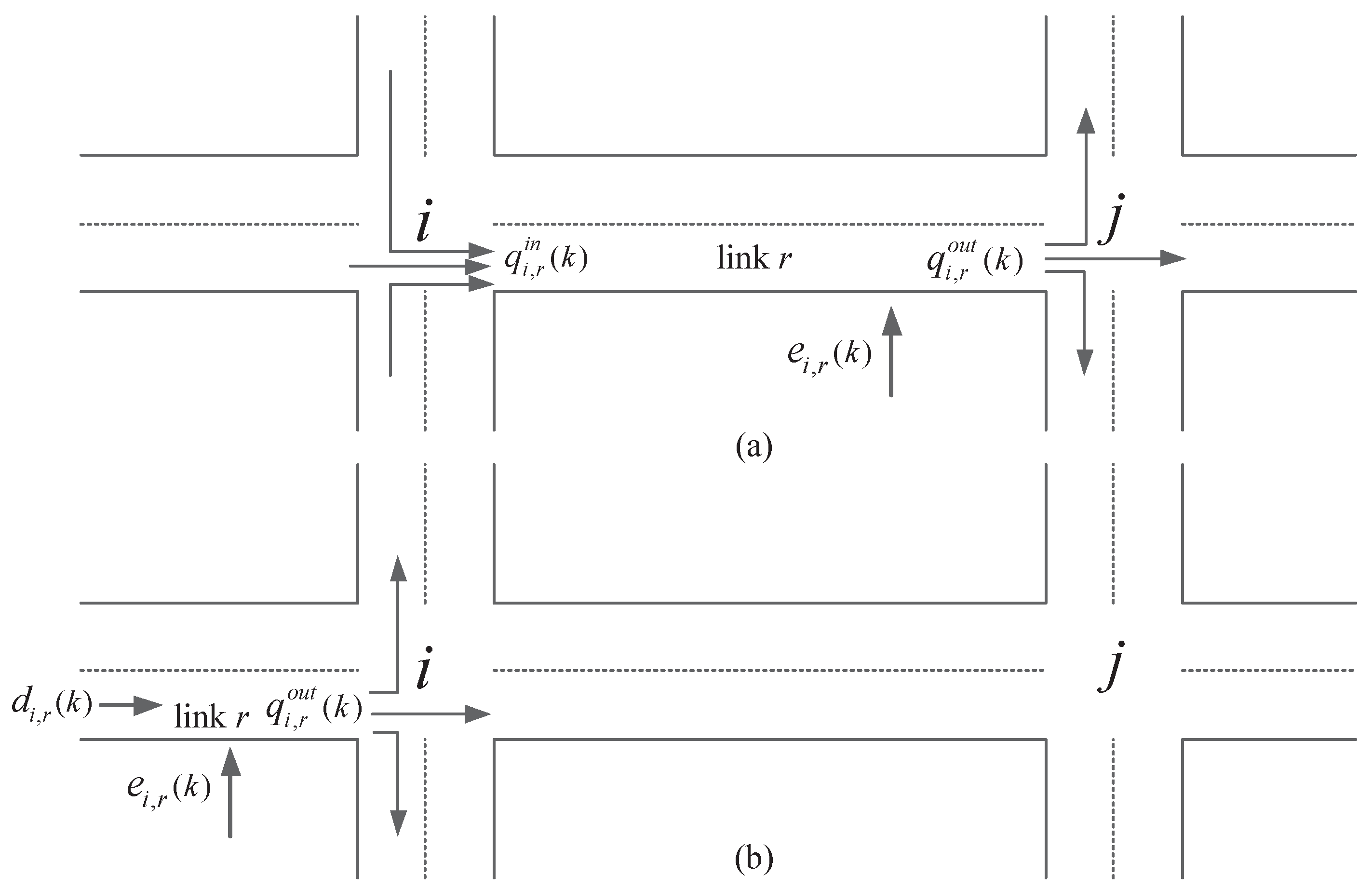
Assume that the link r (as shown in Figure 1a) connects intersection i to intersection j. The traffic dynamics on r can be defined by the following equation:
where () and are the inflow (outflow) and the disturbances (e.g., unexpected traffic fluctuations caused by accidents or parking garage) of link r, respectively. In fact, Equation (1) describes the “vehicle-conservation” on the link r. It should be noted that Guarnaccia [32] has cleverly used the “Kirchhoff Current Law“ to define the “vehicle-conservation” of an intersection.
In addition, the inflow and outflow are calculated by assuming the offset between intersection i and intersection j is equal to zero. They are given by the following two equations:
where denotes the incoming links of the link r. is the set of phases that provides the right of way to the link r of intersection i.
Then, by plugging Equations (2) and (3) into Equation (1), the following state equation can be obtained:
Furthermore, it should be noted that when the link r is one of the incoming links of the UTN (shown in Figure 1b), the inflow should be calculated by the following equation:
where is the traffic demand (vehicles which enter the network through the link r of intersection i). Meanwhile, the Equation (4) should be rewritten as
3. Stochastic MPC-Based Model
3.1. Uncertainty
Due to the complexity and diversity in the real world, uncertainty widely exists in practical engineering problems, and the urban traffic signal control system is no exception. For instance, the traffic demands at the boundary of a specific urban road network, unexpected traffic fluctuations (caused by accidents or parking garage), and the entering (or exiting) traffic flow of a link between the adjacent intersections. As pointed out in [25,27], the variance of traffic demand through the network is the most important. Accordingly, in this paper, we mainly focus on traffic signal modeling and optimization of urban traffic networks with uncertain traffic demand and disturbances.
It is no doubt that the traffic demand (e.g., defined in Equation (5)) varies from day to day and from hour to hour. Assume that we can access the historical traffic information, which was collected during the last few months (or years) and recorded in the database of traffic information management system. Then, by utilizing the previous information and statistic techniques (or tools), we can derive the estimation of the variation tendency. In general, normal distribution can effectively describe the stochastic process in real-world system. Without loss of generality, in this paper, we assume that the traffic demand (e.g., defined in Equation (5)) follows a normal distribution function, i.e.,
where and denote the mean value and variance of , respectively.
Similarly, by using the historical data, we can also approximately derive the probability distribution function of disturbance . In addition, for the convenience of discussion, we define , which follows normal distribution. Assume the mean value and variance of are and ; then, the distribution function of can be defined as
3.2. Constraints
In general, to guarantee the safety of pedestrians and cyclists, there usually exists a green constraint for each phase p of intersection i. In other words, the control variable should satisfy the following constraints:
where and are the predefined minimum and maximum green time, respectively. In addition, the control variables should satisfy the cycle time constraint as defined in Section 2.1.
There can be no doubt that the maximum number () of vehicles in a link r is determined by the length of link r between intersection i and j. Accordingly, to avoid causing serious congestion, the state variable usually should satisfy the following constraints:
Assume that the uncertain demand and the disturbance are independent random variables. Then, according to Equations (7)–(9), we derive easily that the state variable is a random variable that also follows normal distribution. As a result, Equation (11) can be rewritten as
where is the probability distribution function, and is the confidence level that is usually set close to 1. It means that the number of vehicles on the link r of intersection i is set below the maximum allowed with the probability, which is less than . As noted in [27], to avoid the system becoming overly conservative, one does not impose .
3.3. MPC Framework
As one of the most powerful control technologies, since it can efficiently solve control problems with complex constraints, model predictive control (MPC) has been widely used in industrial applications [35]. The main idea of MPC is to access an optimal sequence of future control actions by designing a suitable predictive model. At each control step, only the first element of the optimal sequence is implemented. The horizon is then rolled forward one step and the procedure is repeated with the updated information. Since it has the ability to deal with complex constraints and avoid myopic control schemes in large-scale control problems, various MPC approaches are proposed to coordinate and control the traffic signals for urban traffic network. Furthermore, uncertainties should be reasonably modeled and handled for traffic networks. It is significant to access the optimal signal timing plan of traffic networks. As a result, in the following, we focus on designing a stochastic MPC model to optimize the signal splits for urban traffic networks.
Applying Label (7) to all links of an urban traffic network, we can derive the dynamic equation of the network as follows:
where , , and denote the state vector, control vector, demand vector and disturbance vector, respectively. is the control input matrix, which is used to denote some basic network characteristics (e.g., topology, saturation flows, fixed staging and turning rates), and is the demand matrix.
Assume the length of the prediction horizon length of the control problem is P. For notational simplicity, we define whose element denotes the predicted traffic demand corresponding to one link z of the network. As noted in [27], we can use the historical traffic information to estimate the mean value and variance of . Then, the mean vector and the covariance matrix of can be computed and given in advance as follows:
where is the correlation coefficient between random variables and . Then, the probability density function of the traffic demand of link z is
where is a constant.
Assume the current time index is . The length of the prediction horizon of the control problem is P. Since there may exist uncertainty in the state variable ( ), aiming to minimize the vehicle queue lengths and reduce the oscillation of control variable, we define the control cost function as an expected value model
subject to Labels (10)–(16) and the cycle constraints which are defined in Section 2.1. Q and R are diagonal weighting matrices. The diagonal elements of Q are set equal to . Matrix R reflects the penalty imposed on control effort. Noted that , and m denotes the number of links of the road network.
For notational simplicity, the objective function (18) can be rewritten as
where the state vector . The control vector .
As we can see from Labels (7) and (13), the proposed stochastic MPC-based model is a linear model. It worth noting that, compared with linear models, nonlinear models usually describe the traffic dynamics of road networks more precisely. In future, in order to develop a nonlinear stochastic MPC framework, we can reference the ideas of modeling that were used in the nonlinear MPC models [21,36]. Furthermore, since the emission produced by traffic is one of the important pollution sources, the integrated flow-emission model [37] can also be embedded in the proposed stochastic MPC framework.
4. Optimization Method
4.1. Stochastic Simulation
According to Label (7), the variable could be rewritten as
In addition, applying Label (7) to the whole network, we have Label (13). Then, by defining we can rewrite Label (13) as follows:
Similarly, for , the vector form of chance constraints (12) can be defined as follows:
In order to solve the optimization problem (17), the key issue is to deal with the chance constraints (22). One traditional method to solve the aforementioned problem is transforming the chance constraints (22) to deterministic constraints. However, the results reported in [27] pointed out that the deterministic constraints include multi-integrated terms. The transformed deterministic problem is a special nonlinear problem that can hardly be solved with analytic methods. It is well known that a stochastic simulation method can trace the evolution of variables, which change stochastically (randomly) with certain probabilities. In [28], by using a stochastic simulation method, Liu et al. developed a convenient method to deal with a certain class of uncertain functions.
Based on the above discussion, both the expected value of the objective function defined in Label (17) and the left term in Label (22) can be seen as uncertain functions. Therefore, to calculate the probability value defined in Label (22) and the expected value defined in Label (17), for any and given variable and , we propose a stochastic simulation algorithm (Algorithm 1) to generate input–output data for the uncertain function
where denotes the uncertainty vector corresponding to the whole network. Furthermore, we define and as the probability spaces of and , respectively.
| Algorithm 1 Stochastic Simulation for Uncertain Functions. |
|
4.2. Uncertain Function Approximation
Neural networks (NNs) (also referred to as connectionist systems) are a computational approach, which is inspired by the current understanding of using biological brain to solve problems. It is a class of adaptive systems consisting of a number of simple processing elements, called artificial neurons. Neural networks (NNs) typically consist of multiple layers or a cube design, and the signal path traverses from front to back. An important advantage of NNs is the ability to learn to perform operations, not only for inputs exactly like the training data, but also for new data that may be incomplete or noisy. It has been widely recognized from literature [28,29,30,38] that neural networks (NNs) have the ability to approximate continuous or discontinuous functions and achieve a high speed of operation. Therefore, we decided to train a feedforward NN to approximate the uncertain function (23), aiming at speeding up the solution process of the optimization problem (17).
As pointed out in the user’s guide of the neural network toolbox, a fairly simple neural network can fit any practical function. In this study, we create a single-hidden layer feedforward neural network (SFNN) by using the neural network toolbox of MATLAB (R2016a, MathWorks, Beijing, China). The number of input neurons and that of output neurons are defined as and , which are both decided by the function needed to be approximated. Since the number of input neurons is bigger than that of the output neurons, we set the number of neurons in the hidden layer is proportional to that of the input neurons. That is, is a constant). In order to use the input and output data to train the SFNN, we need to preprocess the data first. In practical application, both input data and output data are usually normalized in the interval .
4.3. Hybrid Intelligent Algorithm
Over the past several decades, genetic algorithms (GAs) have been widely used in the area of management science, operational research and industrial and system engineering. GAs are a class of powerful and broadly applicable stochastic search and optimization methods that really work for many problems that are difficult to be solved by conventional techniques [28,31,39]. As pointed out in [38], the major advantage of GAs is that it is independent of the concave-convex feature of the particular problem being analyzed. GAs require only an objective (fitness) function that can be evaluated for any set of the decision variables. This function can be nonlinear, non-differentiable, or discontinuous. In other words, as a global optimization method, genetic algorithm (GAs) can be implemented to solve the optimization problems (17). As a result, in this paper, we embed the stochastic simulation and neural networks (NNs) into a genetic algorithm (GA) and produce a hybrid intelligent algorithm (HIA). The procedure of the proposed method HIA is summarized as shown in Algorithm 2.
GAs with the basic evaluation, selection, crossover and mutation operators is employed. The first step of GAs is to generate an initial population. According to the objective function defined in Equation (17), it can be easily found that the task of HIA is to get the best control decision serial at each control step . Since the size of each vector of the decision serial is assumed to be equal to m, variables are needed to be optimized at the beginning of each control step. Each variable is coded with L digits of binary number. The length L is determined by the desired representation accuracy [38]. Although there are a number of ways to make selections, a nonlinear selection strategy is adopted in this study. It is worth noting that the feasibility of the offspring individuals (generated by crossover operation or mutation operation) should be checked with a neural network created by Algorithm 1. In addition, to help readers to better understand the main idea of the proposed algorithm HIA, Figure 2 illustrates the scheme diagram of HIA.
| Algorithm 2 Hybrid Intelligent Algorithm |
|
5. Simulation Results
In this paper, we perform simulation experiments on the road network consisting of four intersections. Figure 3 illustrates the basic layouts of the test network. It includes eight links, and four among them ( x1, x2, x5, x6) are input sources where the traffic flow enters the test road network. The lengths of the four input links ( x1, x2, x5, x6) are the same and are equal to 600 m, while about 700 m for the rest links (x3, x4, x7, x8). As shown in Figure 3, each intersection has only two phases. Furthermore, assume that the offset between any two intersections is equal to zero.
Table 1 shows some basic parameters that will be used in the simulation. The turning rates and input traffic flow are illustrated in Table 2 and Figure 4, respectively. The initial state (the number of vehicles on each link at the beginning of the first control step) of the test network is randomly generated. For instance, denotes that the number of vehicles on the link is randomly generated in the interval . Herein, . According to the length of each link and the average length of each vehicle (as defined in Table 1), we set for the link and for the rest links. Herein, denotes the maximum number of vehicles that can be accommodated in a link. For simplicity, we assume that uncertainties only exist on link and link . Furthermore, we assume that the uncertain traffic flow and disturbance are both normally distributed. Aiming to demonstrate the performance of the proposed HIA, the traffic flow and the disturbance shown in Figure 4 are, respectively, assumed to be the mean value of the input flow of and the disturbance of . Furthermore, and are both estimated by historical data. As shown in Table 3, the covariance matrix of and are defined as and , respectively. Note that, for computational simplicity, we assume the covariance matrix and remain unchanged during the whole simulation period. Since previous studies [20,21,22] have shown that it seems reasonable to select the prediction horizon , the experiment results reported in this study are all achieved under the condition that . As a result, the covariance matrix and are three-dimensional matrices. For the measure of solution quality, we report the queue length and the green time of each link in the test network over a simulation period of 20 min (that is six simulation steps).
For the sake of simplicity, let MPC-SPQ denote a deterministic MPC model () that was solved by Sequential Quadratic Programming (SQP), and MPC-GA denotes a deterministic MPC model () that was solved by Genetic Algorithms (GA). In order to demonstrate the performance of the proposed stochastic MPC model that was solved by HIA (abbreviated as MPC-HIA), the performance is compared with MPC-SPQ and MPC-GA. Firstly, the objective functions both of and are the same and defined as and the Equation (18). In addition, except that there are no chance constraints imposed on the queue length (as defined in Equation (12)), the rest constraints of the model are the same as those of the proposed stochastic MPC model. Except for the chance constraints (as defined in Equation (12)) being replaced by the deterministic constraints (as defined in Equation (11)), the rest constraints of the model are the same as those of the proposed stochastic MPC model.
For each control step, based on the mean value and the covariance matrix of (and those of ) we generate 6000 input–output data with Algorithm 1. Then, by using these input–output data and the MATLAB neural network toolbox, we train a feedforward neural network (14 input neurons, one hidden layer with 18 neurons, seven output neurons) for each control step. The mean squared error of the neural network is smaller than . The population size and the maximal generation of GA is set to 50 and 1000, respectively. Selection rate and mutation rate are adopted. In addition, the two genetic algorithms (GAs) (which are used by MPC-HIA and MPC-GA) has the same configuration parameters. It should be noted that all of our simulations are implemented on a personal computer with 32 GB memory and 3.4 GHz, Intel(R) Core CPU i7-6700 processor in the Matlab R2016a environment.
Figure 5 illustrates the queue length of link and that of link at each control step. It can be found that, in terms of the queue length of the link , for the first three control steps, MPC-HIA can achieve a little better (or close) performance than MPC-GA (or MPC-SQP). Beginning with the fourth step, MPC-HIA performs much better than both MPC-SQP and MPC-GA. In addition, in terms of the queue length of the link , MPC-HIA can achieve better performance than both MPC-SQP and MPC-GA at each control step. This may be because, compared with the deterministic MPC models (MPC-SQP) and (MPC-GA), the proposed stochastic MPC model (MPC-HIA) has better ability to handle uncertainties of the test network. More importantly, one can see clearly that the queue length of and that of achieved by MPC-HIA are always below the maximum allowable queue length (a preset value that is proportional to the length of the link) of link and that of during the entire simulation period. The reason for this is that we have imposed two chance constraints on the queue length of the link and that of the in the proposed stochastic model MPC-HIA. However, starting with the fourth control step, the queue length of and that of obtained by MPC-SQP go beyond the upper bound of the allowable queue length.
It should be noted that the upper bound of the (or the maximum) allowable queue length is a preset value, which is proportional to the length of the link. Aiming to avoid the occurrence of queue spill-back, the upper bound of the queue length of (or ) is set equal to of the link length of (or ). As shown in Figure 5, the upper bounds of and are set to 108 (vehicles) and 126 (vehicles), respectively. Another observation on the queue length curves as shown in Figure 5 is that the queue length of (or ) achieved by MPC-SQP continuously increase and go beyond the upper bound since the fourth control step. Especially for the link , the queue length started to mushroom from the third control step onward. These are perhaps caused by two reasons. On one hand, compared with the first two control steps, the input flow of link rapidly increases from the third control step. Meanwhile, vehicles entered into the link and increase quickly. On the other hand, the MPC-SQP did not make a proper allotment of green time to the link and link like the proposed model MPC-HIA did. Since there are constraints that are imposed on the queue lengths of both and , both MPC-HIA and MPC-GA perform better than MPC-SQP.
Figure 6 shows the comparison of the MPC-HIA, MPC-GA and the MPC-SQP on the green time that has been assigned to the link and that of the link at each control step. As shown in Figure 6, during the entire simulation period, the green time of the link (and ) achieved by the proposed model MPC-HIA fluctuates within the minimum and maximum permissible green time (for example 30 s and 90 s). The reason for this may be due to the fact that the input flow and the disturbance are uncertain variables whose mean values vary over each control step (as shown in Figure 4). Furthermore, we can see that the proposed model MPC-HIA can adjust the green time assigned to link (and ) according to the variational traffic demand (or disturbance) and the maximum allowable queue length of the link (and ). This is mainly due to the fact that chance constraint programming was employed into the proposed MPC-HIA model to capture the uncertainties of the network. However, the green time of the link (and ) obtained by the model MPC-SQP shows little changes between any two adjacent control steps. As a result, the queue length of the link (and ) goes beyond the maximum allowable queue length since the fourth control step as shown in Figure 5. It is obvious that results reported in Figure 6 are consistent with those shown in Figure 5.
Figure 7 shows the comparison of the total queue length (during the entire simulation period) of each link for the three models (MPC-HIA, MPC-GA and MPC-SQP). It is not hard to find that the the total lengths of the link achieved by both MPC-HIA and MPC-SQP are almost the same. Meanwhile, the total queue length of the link achieved by MPC-HIA is smaller than that obtained by MPC-SQP. However, for the link , the situation is the reverse. For MPC-GA, a similar conclusion can be reached. The reason is that chance constraints have been imposed on the queue length of link and that of link in the proposed model MPC-HIA. Furthermore, the stochastic MPC model (MPC-HIA) has a better ability to deal with uncertainties than deterministic MPC models—both (MPC-SQP) and (MPC-GA).
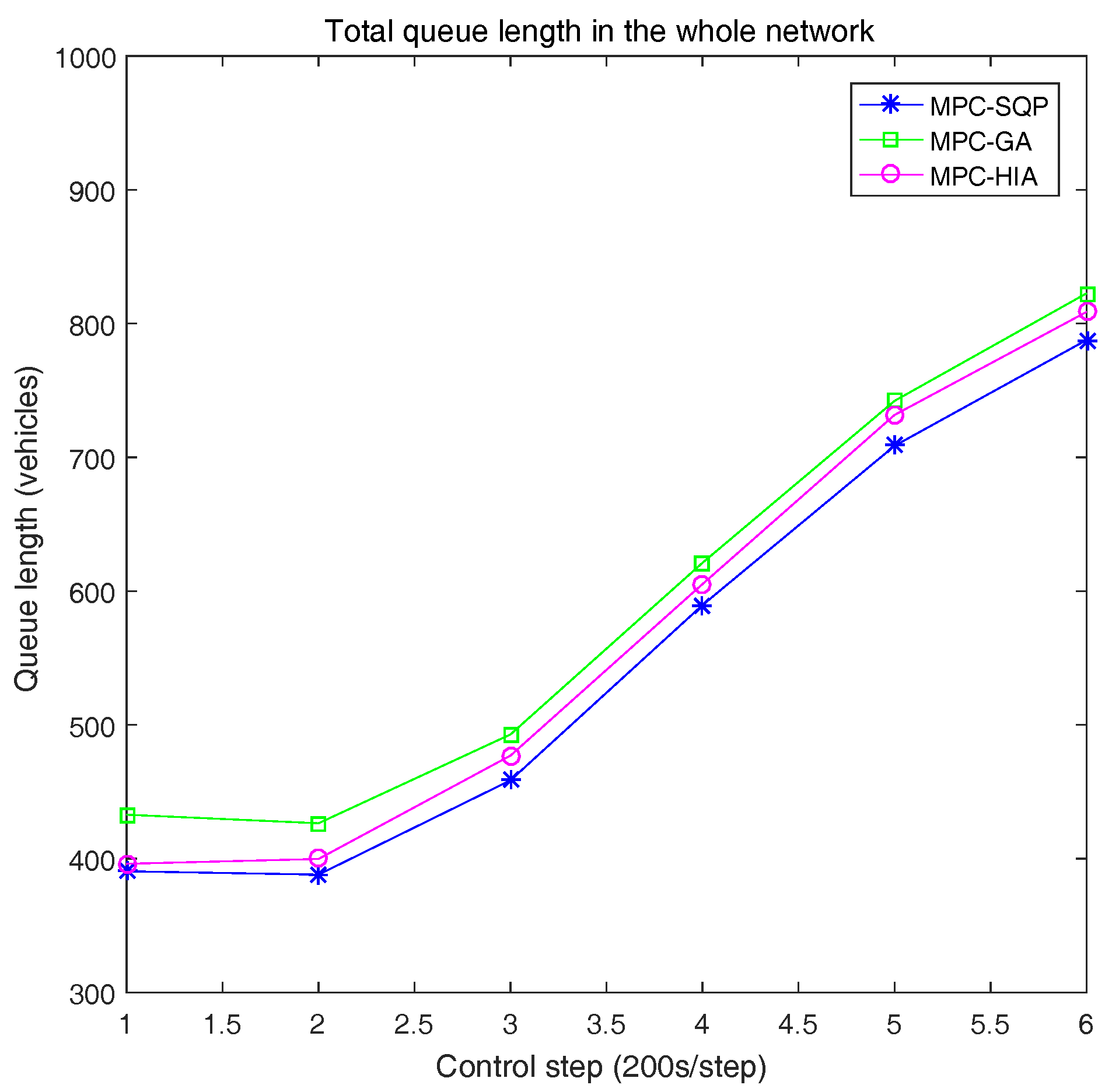
For each control step, the performances of the three models (MPC-HIA, MPC-GA and MPC-SQP), in terms of the total queue length of the network, are illustrated in Figure 8. It can be seen clearly that MPC-SQP performs better than MPC-HIA during the entire simulation period. This may be because, compared with MPC-SQP, there are chance constraints that are imposed on the queue lengths in MPC-SQP. However, MPC-HIA performs better than MPC-GA over the whole simulation period. This is perhaps due to the fact that the stochastic MPC model (MPC-HIA) has better performance than the deterministic MPC model (MPC-GA) in terms of dealing with uncertainties, which are imposed on link and link .
In addition, to evaluate the performance of computational cost, we report the average computation time of ten independent runs for solving the MPC optimization problem with the three methods (MPC-SQP, MPC-GA and MPC-HIA). The computational time per simulation of MPC-SQP, MPC-GA and MPC-HIA are 1.653 s, 460 s and 16,932.5 s, respectively. It is obviously that both MPC-SQP and MPC-GA perform much better than MPC-HIA. The reason for this may be that, compared with deterministic MPC models (MPC-SQP) and (MPC-GA), the stochastic MPC model (MPC-HIA) has much higher computational complexity.
To summarize, it has been shown that the proposed model MPC-HIA performs better than MPC-SQP and MPC-GA in terms of avoiding queue spillback under uncertain conditions (e.g., the link has uncertain traffic demands or disturbances). However, both MPC-SQP and MPC-GA perform much better than the proposed model MPC-HIA in terms of the performance of computational cost. This may be because the stochastic MPC model (MPC-HIA) has a better ability to deal with uncertainties than deterministic MPC models—both (MPC-SQP) and (MPC-GA). Meanwhile, since there are chance constraints and uncertain objective function in the stochastic MPC model (MPC-HIA), MPC-HIA has higher computational complexity than MPC-SQP and MPC-GA.
6. Conclusions
In this paper, we have proposed a stochastic MPC model for urban traffic signal coordination and control. Under the framework of the stochastic MPC model, we use chance constraint programming to model the uncertain traffic demands and uncertain disturbances of the road network. The detailed mathematical description of the model has been provided. Since the proposed model is a stochastic MPC model with chance constraints, by embedding the stochastic simulation and neural networks (NNs) into a genetic algorithms (GA), we propose a hybrid intelligent approach to solve the stochastic model. In addition, aiming to demonstrate the performance of the proposed stochastic MPC model, which was solved by HIA (abbreviated as MPC-HIA), the performance are compared with a deterministic MPC model (M1), which was solved by Sequential Quadratic Programming (SQP) and a deterministic MPC model (M2), which was solved by a Genetic Algorithm (GA). Numerical simulations illustrate that, compared with the deterministic MPC model, the proposed stochastic MPC model has a better ability to deal with uncertainties and avoid queue spill-back in urban road networks.
In future research, additional testing in different types (or sizes) of networks and with different arrival types (or probability distribution model) should be investigated. In order to reduce the computational cost, we can design hierarchical or distributed control strategies and algorithms to reduce the computational complexity of the stochastic MPC model. The mismatch between the proposed MPC model and real traffic systems will be considered. Furthermore, other performance indexes (e.g., the one which can reflect the fuel consumption or vehicle emissions) can also be embedded in the objective function of the proposed stochastic MPC model.
Acknowledgments
The authors would like to acknowledge the financial support of the National Natural Science Foundation of China under Grants No. 61603154 and No. 61374066, and by the Zhejiang Provincial Natural Science Foundation of China under Grant No. LY15F030021.
Author Contributions
Bao-Lin Ye, Weimin Wu and Huimin Gao conceived, designed and performed the experiments; Yixia Lu, Qianqian Cao and Lijun Zhu analyzed the data; and Bao-Lin Ye wrote the paper.
Conflicts of Interest
The authors declare no conflict of interest.
References
- Papageorgiou, M.; Diakaki, C.; Dinopoulou, V.; Kotsialos, A.; Wang, Y. Review of road traffic control strategies. Proc. IEEE 2003, 91, 2043–2067. [Google Scholar] [CrossRef]
- Porche, I.; Lafortune, S. Adaptive Look-ahead Optimization of Traffic Signals. J. Intell. Transp. Syst. 1999, 4, 209–254. [Google Scholar]
- Xie, X.F.; Smith, S.F.; Lu, L.; Barlow, G.J. Schedule-driven intersection control. Transp. Res. C Emerg. Technol. 2012, 24, 168–189. [Google Scholar] [CrossRef]
- Gartner, N.H.; Pooran, F.J.; Andrews, C.M. Optimized policies for adaptive control strategy in real-time traffic adaptive control systems: Implementation and field testing. Transp. Res. Rec. J. Transp. Res. Board 2002, 1811, 148–156. [Google Scholar] [CrossRef]
- Robertson, D.I.; Bretherton, R.D. Optimizing networks of traffic signals in real time: The SCOOT method. IEEE Trans. Veh. Technol. 1991, 40, 11–15. [Google Scholar] [CrossRef]
- Lowrie, P. The Sydney coordinated adaptive traffic system-principles, methodology, algorithms. In Proceedings of the International Conference on Road Traffic Signaling, London, UK, 30 March–1 April 1982; pp. 60–67. [Google Scholar]
- Gartner, N.H. OPAC: A demand-responsive strategy for traffic signal control. Transp. Res. Rec. J. Transp. Res. Board 1983, 906, 75–81. [Google Scholar]
- Henry, J.J.; Farges, J.L.; Tuffal, J. The PRODYN real time traffic algorithm. In Proceedings of the 4th Ifac/ifip/ifors Conference on Control in Transportation Systems, Baden-Baden, Germany, 20–22 April 1983; pp. 305–310. [Google Scholar]
- Sen, S.; Head, K.L. Controlled optimization of phases at an intersection. Transp. Sci. 1997, 31, 5–17. [Google Scholar] [CrossRef]
- Gazis, D.C.; Potts, R.B. The oversaturated intersection. In International Symposia on Traffic Theory, 2nd ed.; International Business Machines Corporation: London, UK, 1963; pp. 221–237. [Google Scholar]
- Diakaki, C.; Papageorgiou, M.; Aboudolas, K. A multivariable regulator approach to traffic-responsive network-wide signal control. Control Eng. Pract. 2002, 10, 183–195. [Google Scholar] [CrossRef]
- Aboudolas, K.; Papageorgiou, M.; Kosmatopoulos, E. Store-and-forward based methods for the signal control problem in large-scale congested urban road networks. Transp. Res. C Emerg. Technol. 2009, 17, 163–174. [Google Scholar] [CrossRef]
- Aboudolas, K.; Papageorgiou, M.; Kouvelas, A.; Kosmatopoulos, E. A rolling-horizon quadratic-programming approach to the signal control problem in large-scale congested urban road networks. Transp. Res. Part C Emerg. Technol. 2010, 18, 680–694. [Google Scholar] [CrossRef]
- Tettamanti, T.; Varga, I. Distributed traffic control system based on model predictive control. Civ. Eng. 2010, 54, 3–9. [Google Scholar] [CrossRef]
- De Oliveira, L.B.; Camponogara, E. Multi-agent model predictive control of signaling split in urban traffic networks. Transp. Res. C Emerg. Technol. 2010, 18, 120–139. [Google Scholar] [CrossRef]
- Camponogara, E.; Scherer, H.F. Distributed optimization for model predictive control of linear dynamic networks with control-input and output constraints. IEEE Trans. Autom. Sci. Eng. 2011, 8, 233–242. [Google Scholar] [CrossRef]
- Lin, S.; De Schutter, B.; Xi, Y.; Hellendoorn, H. Efficient network-wide model-based predictive control for urban traffic networks. Trans. Res. C Emerg. Technol. 2012, 24, 122–140. [Google Scholar] [CrossRef]
- Lin, S.; De Schutter, B.; Xi, Y.; Hellendoorn, H. Fast model predictive control for urban road networks via MILP. IEEE Trans. Intell. Transp. Syst. 2011, 12, 846–856. [Google Scholar] [CrossRef]
- Zhou, X.; Lu, Y. Coordinate model predictive control with neighbourhood optimisation for a signal split in urban traffic networks. IET Intell. Transp. Syst. 2012, 6, 372–379. [Google Scholar] [CrossRef]
- Ye, B.L.; Wu, W.; Zhou, X.; Mao, W.; Li, J. A signal split optimization approach based on model predictive control for large-scale urban traffic networks. In Proceedings of the 2013 IEEE International Conference on Automation Science and Engineering (CASE), Madison, WI, USA, 17–20 Augest 2013; pp. 904–909. [Google Scholar]
- Ye, B.L.; Wu, W.; Mao, W. Distributed Model Predictive Control Method for Optimal Coordination of Signal Splits in Urban Traffic Networks. Asian J. Control 2015, 17, 775–790. [Google Scholar] [CrossRef]
- Ye, B.L.; Wu, W.; Li, L.; Mao, W. A hierarchical model predictive control approach for signal splits optimization in large-scale urban road networks. IEEE Trans. Intell. Transp. Syst. 2016, 17, 2182–2192. [Google Scholar] [CrossRef]
- Yin, Y. Robust optimal traffic signal timing. Transp. Res. B Methodol. 2008, 42, 911–924. [Google Scholar] [CrossRef]
- Zhang, L.; Yin, Y.; Lou, Y. Robust signal timing for arterials under day-to-day demand variations. Transp. Res. Rec. J. Transp. Res. Board 2010, 2010, 156–166. [Google Scholar] [CrossRef]
- Tamas, T.; Tamas, L.; Balazs, K.; Tamas, P.; Istvan, V. Robust control for urban road traffic networks. IEEE Trans. Intell. Transp. Syst. 2014, 15, 385–398. [Google Scholar]
- Liu, S.; Sadowska, A.; Frejo, J.R.D.; Núñez, A.; Camacho, E.F.; Hellendoorn, H.; De Schutter, B. Robust receding horizon parameterized control for multi-class freeway networks: A tractable scenario-based approach. Int. J. Robust Nonlinear Control 2016, 26, 1211–1245. [Google Scholar] [CrossRef]
- Zhou, X.; Ye, B.L.; Lu, Y.; Xiong, R. A Novel MPC with Chance Constraints for Signal Control in Urban Traffic Networks. In Proceedings of the 19th World Congress of International Federation of Automatic Control, Cape Town, South Africa, 24–29 August 2014; pp. 11311–11317. [Google Scholar]
- Liu, B. Theory and Practice of Uncertain Programming, 2nd ed.; Springer: Berlin, Germany, 2002. [Google Scholar]
- Wang, T.; Gao, H.; Qiu, J. A combined adaptive neural network and nonlinear model predictive control for multirate networked industrial process control. IEEE Trans. Neural Netw. Learn. Syst. 2016, 27, 416–425. [Google Scholar] [CrossRef] [PubMed]
- Su, J.; Liu, J.; Thomas, D.B.; Cheung, P.Y. Neural Network Based Reinforcement Learning Acceleration on FPGA Platforms. ACM SIGARCH Comput. Archit. News 2017, 44, 68–73. [Google Scholar] [CrossRef]
- Ganjehkaviri, A.; Jaafar, M.M.; Hosseini, S.E.; Barzegaravval, H. Genetic algorithm for optimization of energy systems: Solution uniqueness, accuracy, Pareto convergence and dimension reduction. Energy 2017, 119, 167–177. [Google Scholar] [CrossRef]
- Guarnaccia, C. Acoustical noise analysis in road intersections: A case study. In Proceedings of the 11th WSEAS International Conference on Acoustics and Music: Theory and Applications, Iasi, Romania, 13–15 June 2010; pp. 13–15. [Google Scholar]
- Park, B.; Messer, C.; Urbanik, T. Traffic signal optimization program for oversaturated conditions: Genetic algorithm. Transp. Res. Rec. J. Transp. Res. Board 2002, 1683, 133–142. [Google Scholar] [CrossRef]
- Arel, I.; Liu, T.; Urbanik, A.; Kohls, G. Reinforcement learning-based multi-agent system for network traffic signal control. IET Intell. Transp. Syst. 2010, 4, 128–135. [Google Scholar] [CrossRef]
- Camacho, E.F.; Alba, C.B. Model Predictive Control; Springer: Berlin, Germany, 2013. [Google Scholar]
- Portilla, C.; Valencia, F.; Espinosa, J.; Núñez, A.; De Schutter, B. Model-based predictive control for bicycling in urban intersections. Transp. Res. C Emerg. Technol. 2016, 70, 27–41. [Google Scholar] [CrossRef]
- Jamshidnejad, A.; Papamichail, I.; Papageorgiou, M.; De Schutter, B. A mesoscopic integrated urban traffic flow-emission model. Transp. Res. C Emerg. Technol. 2017, 75, 45–83. [Google Scholar] [CrossRef]
- Alaa, H.A.; Richard, C.P. Optimal design of aquifer cleanup systems under uncertainty using a neural network and a genetic algorithm. Water Resour. Res. 1999, 35, 2523–2532. [Google Scholar] [CrossRef]
- Whitley, D. A genetic algorithm tutorial. Stat. Comput. 1994, 4, 65–85. [Google Scholar] [CrossRef]
Figure 1.
Traffic dynamics on a link. (a) dynamics on a non-input link; (b) dynamics on an input link.
Figure 1.
Traffic dynamics on a link. (a) dynamics on a non-input link; (b) dynamics on an input link.

Figure 2.
Scheme diagram of the proposed algorithm Hybrid Intelligent Algorithm (HIA).

Figure 3.
Test network with signalized intersections.
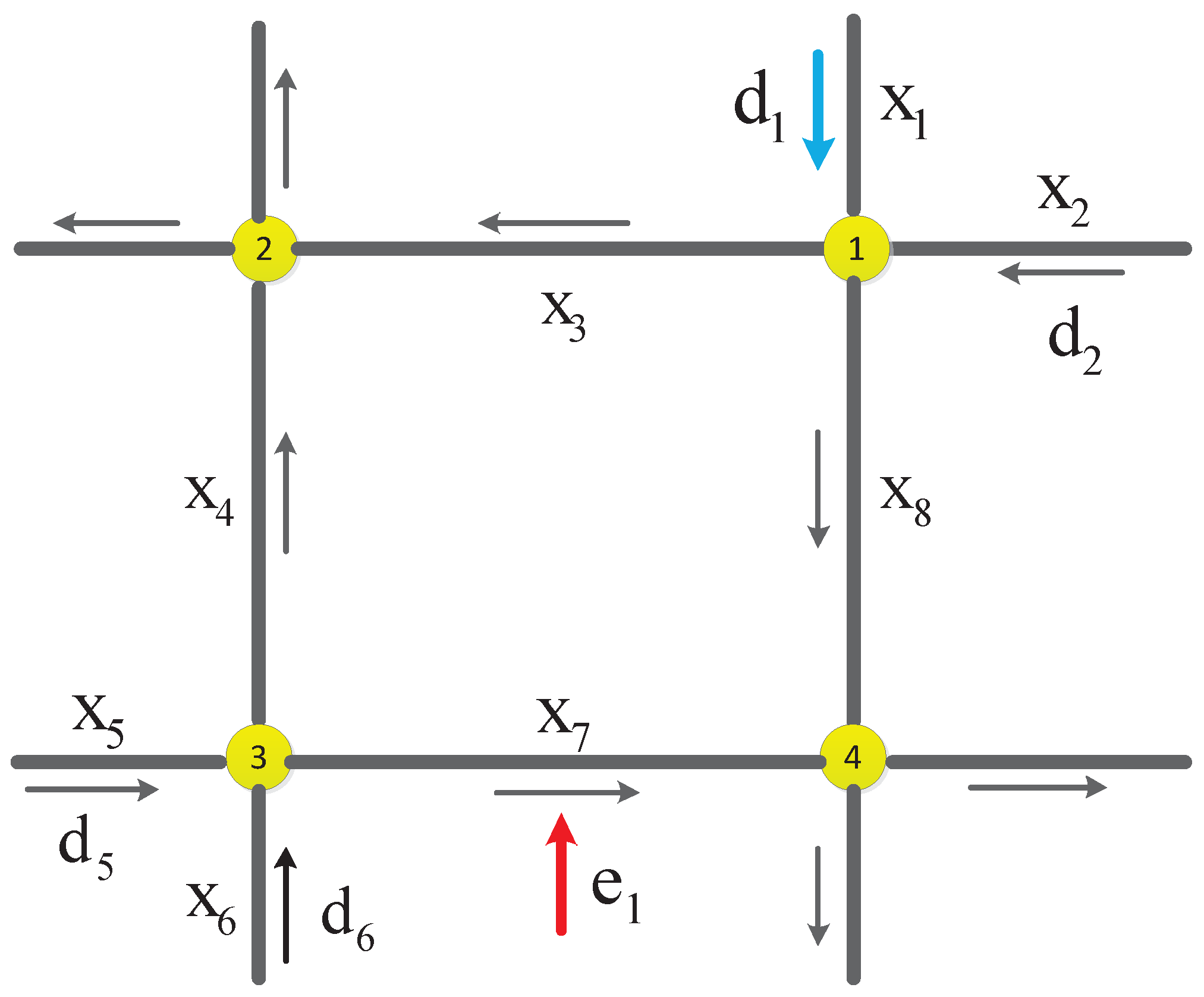
Figure 4.
Input traffic flow and disturbance of the test network.

Figure 5.
Comparison of the queue length of and at each control step.

Figure 6.
Comparison of the green time of and at each control step.
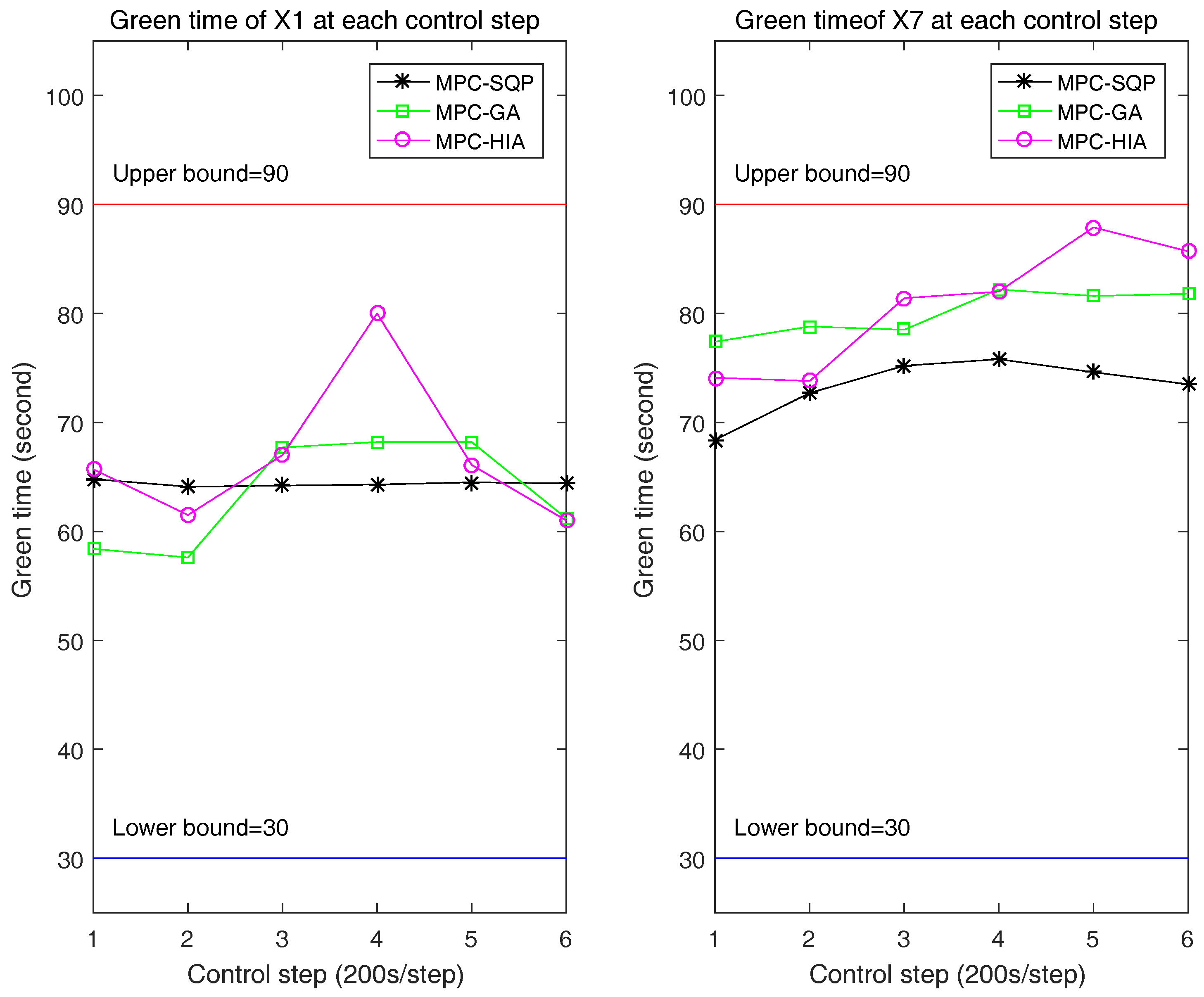
Figure 7.
Comparison of the queue length of each link.

Figure 8.
Comparison of the queue length at each control step.

Table 1.
Simulation parameters.
| Variable | Parameter | Simulation Value |
|---|---|---|
| C | common cycle time | 120 s |
| L | lost time | 8 s |
| S | saturation flow rate | 3600 veh/h |
| T | control interval | 200 s |
| l | average vehicle length | 5 m |
| P | prediction horizon length | 3 |
| u | constraint on green time |
Table 2.
Turning rates for the test road network.
| x1 | x2 | x3 | x4 | x5 | x6 | x7 | x8 | |
|---|---|---|---|---|---|---|---|---|
| x1 | - | - | 0.3 | - | - | - | - | 0.7 |
| x2 | - | - | 0.8 | - | - | - | - | 0.2 |
| x3 | - | - | - | - | - | - | - | - |
| x4 | - | - | - | - | - | - | - | - |
| x5 | - | - | - | 0.6 | - | - | 0.4 | - |
| x6 | - | - | - | 0.2 | - | - | 0.8 | - |
| x7 | - | - | - | - | - | - | - | - |
| x8 | - | - | - | - | - | - | - | - |
Table 3.
Covariance matrix of uncertain demand and disturbance.
| Uncertain Variable | |||||||
| 16128 | 0 | 108 | |||||
| 0 | 6912 | 216 | 108 | ||||
| 10368 | 108 | 162 | |||||
© 2017 by the authors. Licensee MDPI, Basel, Switzerland. This article is an open access article distributed under the terms and conditions of the Creative Commons Attribution (CC BY) license (http://creativecommons.org/licenses/by/4.0/).
Share and Cite
MDPI and ACS Style
Ye, B.-L.; Wu, W.; Gao, H.; Lu, Y.; Cao, Q.; Zhu, L. Stochastic Model Predictive Control for Urban Traffic Networks. Appl. Sci. 2017, 7, 588. https://doi.org/10.3390/app7060588
AMA Style
Ye B-L, Wu W, Gao H, Lu Y, Cao Q, Zhu L. Stochastic Model Predictive Control for Urban Traffic Networks. Applied Sciences. 2017; 7(6):588. https://doi.org/10.3390/app7060588
Chicago/Turabian StyleYe, Bao-Lin, Weimin Wu, Huimin Gao, Yixia Lu, Qianqian Cao, and Lijun Zhu. 2017. "Stochastic Model Predictive Control for Urban Traffic Networks" Applied Sciences 7, no. 6: 588. https://doi.org/10.3390/app7060588
Note that from the first issue of 2016, this journal uses article numbers instead of page numbers. See further details here.