Target Localization in Underwater Acoustic Sensor Networks Using RSS Measurements


1
Faculty of Electrical Engineering and Computer Science, Ningbo University, Ningbo 315211, China
2
Xiamen Key Laboratory of Mobile Multimedia Communications, Huaqiao University, 668 Jimei Avenue, Xiamen 361021, China
*
Author to whom correspondence should be addressed.
Appl. Sci. 2018, 8(2), 225; https://doi.org/10.3390/app8020225
Submission received: 28 November 2017
/
Revised: 26 January 2018
/
Accepted: 29 January 2018
/
Published: 1 February 2018
(This article belongs to the Special Issue Underwater Acoustics, Communications and Information Processing)
Abstract
:This paper addresses the target localization problems based on received signal strength (RSS) measurements in underwater acoustic wireless sensor network (UWSN). Firstly, the problems based on the maximum likelihood (ML) criterion for estimating target localization in cases of both known and unknown transmit power are respectively derived, and fast implementation algorithms are proposed by transforming the non-convex problems into a generalized trust region subproblem (GTRS) frameworks. A three-step procedure is also provided to enhance the estimation accuracy in the unknown target transmit power case. Furthermore, the Cramer–Rao lower bounds (CRLBs) in both cases are derived. Computer simulation results show the superior performance of the proposed methods in the underwater environment.
1. Introduction
Target localization in underwater acoustic wireless sensor network (UWSN) has attracted much attention in recent years due to its wide applications in such fields as data collection, pollution monitoring, offshore exploration, disaster prevention, target tracking, assisted navigation, and military surveillance [1,2,3]. In UWSN, target localization is often performed by using such measurement information as time-of-arrival (ToA), time-different-of-arrival (TDoA), angle-of-arrival (AoA), and received-signal-strength (RSS). However, localization based on ToA and TDoA requires careful timing and synchronization, and the costs are high, especially in underwater acoustic environmental conditions [4,5,6]. Additionally, as AoA relies on a direct line-of-sight path from the target node to anchor nodes, it will cause large errors in AoA measurements in multi-path underwater acoustic (UWA) transmission environments [7,8]. Therefore, RSS-based target localization is preferred by researchers due to its low complexity and easy implementation [9,10,11,12]. Based on the received signal strength measurements, the maximum likelihood (ML) method is used to estimate the target position [13], and this method is robust in underwater environments. Although the ML estimator has asymptotically optimal performance, it is non-convex and has multiple local optimal solutions. Moreover, its performance depends highly on the initial solution and obtains bad results if a poor initialization is provided. In [9], the authors propose a fast iteration algorithm by using a triangulation method based on RSS measurements. In [11], the authors discuss the convex optimization method for target localization in UWSN, while the propagation model is still the terrestrial acoustic wave model. Two convex methods based respectively on RSS-based and frequency-dependent differential approaches in UWSN have been proposed [12]. A hybrid localization method was investigated by combining ToA and RSS measurements [10]. This method provides better performance by exploiting the benefits of combined measurements of the radio signal in the assumption that the RSS measurements are known in advance.
In this paper, target localization methods for the cases of both known and unknown target transmit power are proposed. Firstly, the general target localization problems based on the ML criterion are formed, and the new weighted least square (WLS) problems are then derived using approximation techniques. These non-convex estimators are then transformed into a generalized trust region subproblem (GTRS) framework [14], which are solved in an efficient way. Furthermore, a three-step procedure is used to enhance the estimation accuracy of the target localization in the unknown target transmit power case. Finally, the closed-form expressions of the Cramer–Rao lower bounds (CRLBs) in both known and unknown target transmit power cases are derived.
The remainder of this paper is organized as follows. In Section 2, the RSS measurement model for locating a single target node is briefly introduced, and the non-convex target localization problem is formulated. Section 3 derives the proposed methods in both the known and unknown transmit power cases. In Section 4, complexity analysis is carried out. Computer simulation comparisons of the discussed methods are presented in Section 5. The CRLBs in both known and unknown transmit power cases are derived in Section 6. In Section 7, the main conclusions are drawn. Finally, Section 8 points out the idea of further research.
2. The System Model
Consider an UWSN with N anchor nodes and one target node in a two-dimensional () localization scenario, where the locations of anchor nodes, noted as , are known, while the location of the target node, noted as , is unknown. For simplicity and without loss of generality, we assume that the anchor nodes are equipped with omnidirectional antennas. Under a centralized processing mode, all sensors convey their RSS measurements with respect to the target node to the central processor. We assume that the locations of all the nodes are supposed to be unchanged during the computation period [11,15]. Figure 1 shows the i-th sensoring link in the UWSN model.
For , the RSS of the UWA propagation between the i-th anchor node and the target node is measured in dBm and has the log-normal shadowing model as follows [12]:
where is the Euclidean distance, is a zero-mean Gaussian random variable with covariance matrix that represents the log-normal shadowing effect, is the reference power at the reference distance , is the path-loss exponent between 2 and 4 according to different propagation environments, and is the absorption coefficient that can be obtained from Thorp’s formula as a function of signal frequency f in dB/km, which is as follows [16]:
Let be the collection vector of Gaussian random variables with a symmetric and positive-definite covariance matrix as follows:
where is the correlation coefficient of any two different links between i and j to the target node for . It is known from Equation (3) that can be transformed into white noise using the Cholesky decomposition as with lower-triangular matrix . This implies a linear transformation , where , and is the order-N unity matrix [17].
Let be the vector of observations given by Equation (1). The joint probability density function (PDF) of , conditioned on a given , has the following form
where , with each component
Therefore, the joint ML estimation of the target location can be formulated as
In the special case where , which corresponds to added white Gaussian noise, the estimation can be reduced as
3. The Proposed Methods
In this section, we provide an approximation method that can transform the ML estimator into a GTRS problem. Without loss of generality, we assume that noise is sufficiently small, and let m [12,15]. From Equation (1), we have the following approximation expression
Let be the exponent of the second factor on the right hand side of Equation (7). It was shown in [12,18] that, when the absorption coefficient is sufficiently small, the absorption term can be relatively small ( ), especially in deep water; then, . Therefore, for a sufficiently small , it is reasonable to approximate this factor by using the first-order Taylor expansion about as follows:
where the higher-order terms are omitted.
By substituting Equation (8) into Equation (7), the distance between the i-th anchor and the target node can be further approximated in the following form:
where , and .
3.1. Target Localization in the Known Transmit Power Case
In the known transmit power case, is assumed to be known in the centralized localization, so is a constant that depends only on the path-loss exponent . Given , , , and the coefficients , the target node localization can be determined from Equation (9). Next, we can rewrite Equation (9) as
Based on Equation (10), we propose the following WLS estimation problem:
The above WLS estimator is still a non-convex optimization problem. In the following section, we can transform Equation (11) into an equivalent quadratic programming problem with a quadratic constraint whose global solution can be computed efficiently [19].
Although Equation (12) is still non-convex, both the objective function and the constraint in Equation (12) are quadratic. This is a typical quadratic programming problem with quadratic constraint and can be solved using the bisection method [19]. In the sequel, this method is noted as “WLS-K”(weighted least square–known).
3.2. Target Localization in the Unknown Transmit Power Case
In most practical applications, the target transmit power is unknown. Therefore, the related or in Equation (11) is unknown. Therefore, the method proposed in Section 3.1 cannot be used directly in this case. To cope with the difficulties caused by this additional unknown parameter, we developed the following method.
Furthermore, Equation (15) can be rewritten as
We divide from both the numerator and denominator of the second term on the right hand side of Equation (16), yielding
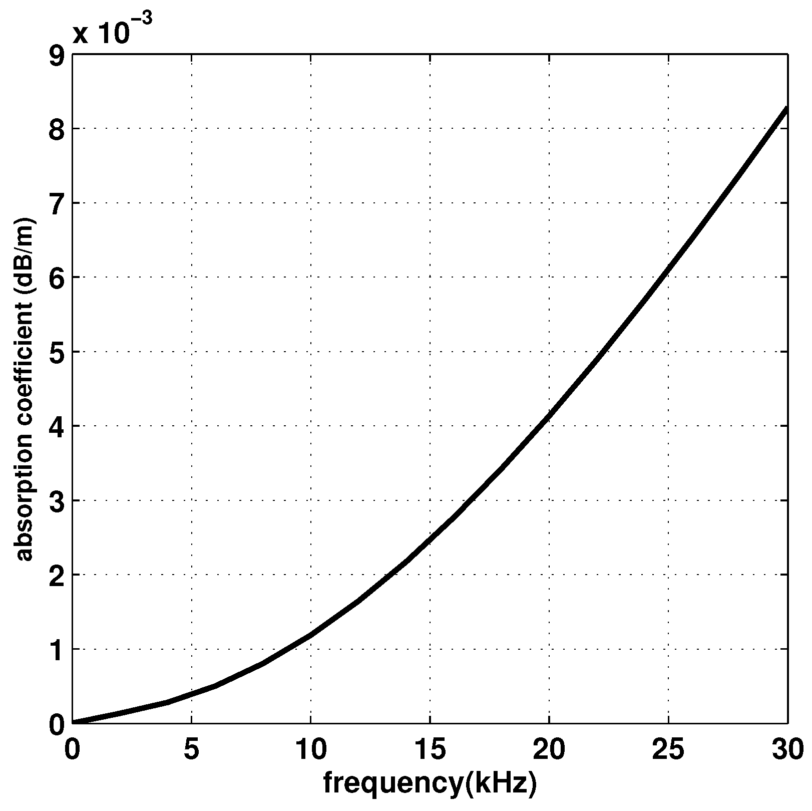
Let , in which is related to the frequency, is related to the signal power, is a constant, and is an independent unknown parameter. We will verify that in most UWSN environments. Figure 2 is the versus the frequency band 0–30 kHz, within which most acoustic systems operate [20,21,22]. The figure shows that . Figure 3 shows versus the transmit signal power when takes three different values (in dB/m). The figure shows that in this case. Therefore, when the absorption coefficient is sufficiently small, it is reasonable to approximate Equation (17) by using the first-order Taylor expansion about as follows:
As in the previous section, squaring both sides of Equation (19), we have
Thus, we can obtain the following WLS problem:
Equation (22) is still non-convex, but both the objective function and the constraint are quadratic and can therefore be solved by using the bisection method [19], as discussed in Section 3.1.
In fact, we can further improve localization performance in the unknown transmit power case. To do so, first, we solve Equation (22) to obtain the initial location estimate of target node , , and then use this estimate to search for the ML estimate of the transmit power , . Finally, with the estimated , the problem is transformed into the localization in the known transmit power case. Hence, we form the following three-step procedure:
We label this method as “WLS-U”(weighted least square–unknown).
4. Complexity Analysis
There is an inherent trade-off between estimation accuracy and implementation complexity among all proposed methods. The method for the worst-case complexity of the mixed SD/SOCP [23] is used to analyze the complexities of the proposed and other discussed methods in this paper. Table 1 shows that the computational complexity of the discussed methods mainly depend on the network size, i.e., the number of anchor nodes.
From Table 1, we see that the proposed methods have less complexity.
5. Cramer–Rao Lower Bound Analysis
The Cramer–Rao lower bounds of the target localization in UWSN are derived in this section to compare the performance of the proposed methods. Let , and , where , and , with
Thus, the Cramer-Rao lower bounds (CRLBs) of the target node location in both known and unknown transmit power cases, i.e., CRLB-K (Cramer–Rao lower bound-known) and CRLB-U (Cramer–Rao lower bound-unknown) can respectively be written as
For detailed derivations, please refer to the Appendix.
6. Simulation Results and Analysis
In this section, computer simulation results are used to compare the performance of the proposed methods with the SDP method (RSS-based approach) in [12] in underwater acoustic environments. The propagation model, Equation (1), is used to generate the range measurements. The anchor nodes and target node are assumed to be randomly located at a square region 100 m × 100 m in each Monte carlo (Mc) run. Unless otherwise stated, the reference distance is set to be m, the reference power is dBm, the maximum number of steps in the bisection procedure is , and the path-loss exponent is fixed as , which corresponds to an UWA spherical spreading case. Different values of are given in each figure. The noise correlation coefficient for . Three thousand Monte carlo runs are used to compute the root mean square error (RMSE) defined as RMSE , where is the estimated location in the i-th Monte Carlo run. The SDP is solved using the MATLAB package CVX (Version 2.1, Stanford University, Stanford, CA, USA, 2014) [24], where the solver is SeDuMi (Version 1.02, Tilburg University, Tilburg, Netherlands, 1999) [25]. The corresponding ML problems are solved by the MATLAB function “Isqnonlin,” which adopts the Levenberg–Marquardt algorithm.
Figure 4 compares the RMSE versus the standard derivation . It is observed that the RMSE grows in nature as the standard derivation increases for all the methods. The proposed localization method WLS-K in the case of known transmit power provides superior performance over the SDP method, and approximates the CRLB-K even when the standard derivation increases. Furthermore, to the best of the authors’ knowledge, few people has discussed localization methods based on a UWA RSS propagation model in unknown transmit power cases in UWSN. Therefore, we compared the performance of the proposed WLS-U with CRLB-U in this case. The results show that the proposed method in this case also maintains an optimal performance.
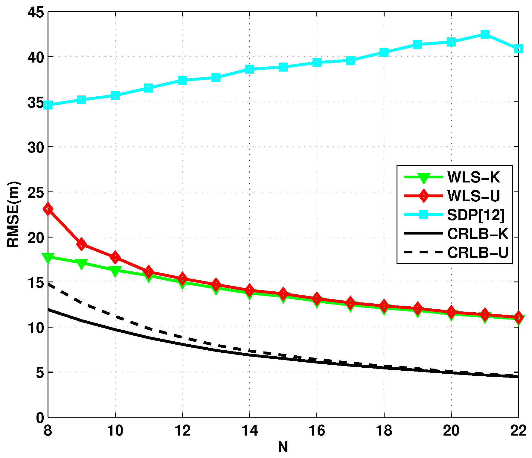
Figure 5 compares the RMSE versus the number N of the anchor nodes. As predicted, the RMSE decreases in nature as N increases for both the WLS-K and WLS-U methods. The figure also shows that adding more anchor nodes in the network can enhance the performance of the proposed methods and outperform the SDP method for all chosen N. Moreover, the performance of WLS-K is slightly better than WLS-U.
Figure 6 depicts the cumulative density function (CDF) of localization comparison versus mean error (ME) among the discussed methods. The figure shows that the proposed methods show an improvement in performance compared with the SDP method.
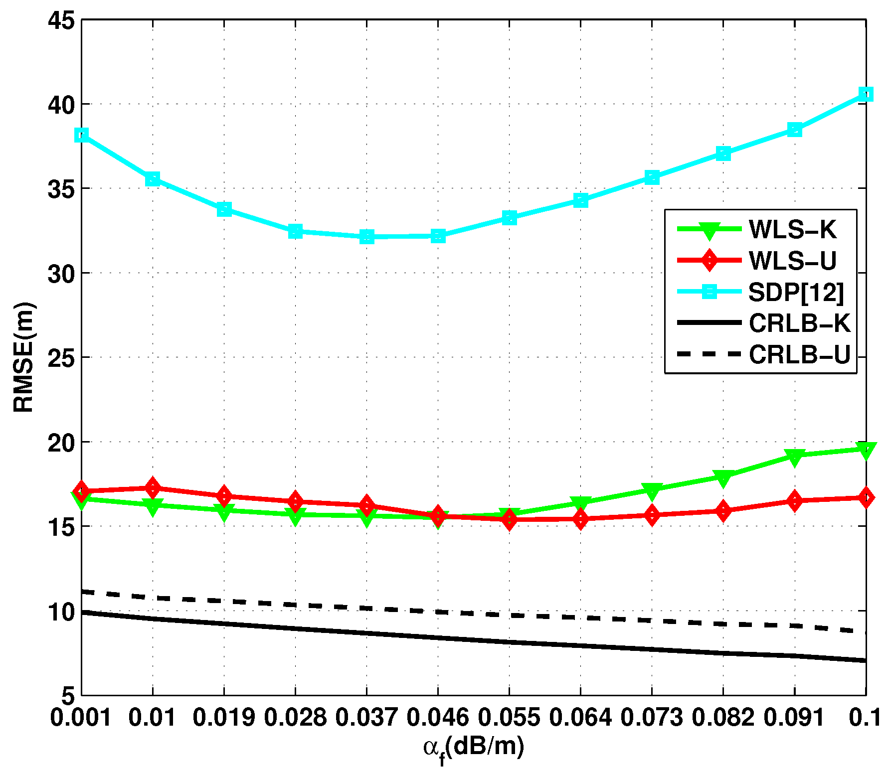
Figure 7 compares the RMSE versus the absorption coefficient . The figure shows that the RMSE crease in with the increase in absorption coefficient for the discussed methods, and WLS-K method shows a performance that is superior to the SDP method. Furthermore, the gap between the WLS-K method and the WLS-U method is small. This is due to the fact that, in the proposed WLS-U method, with some approximation, the unknown transmit power can be estimated from the GTRS optimization problem, Equation (22). In this case, the problem is transformed into the same problem in the known transmitter power case. The results show that the proposed methods have robust performance for from to dB/m.
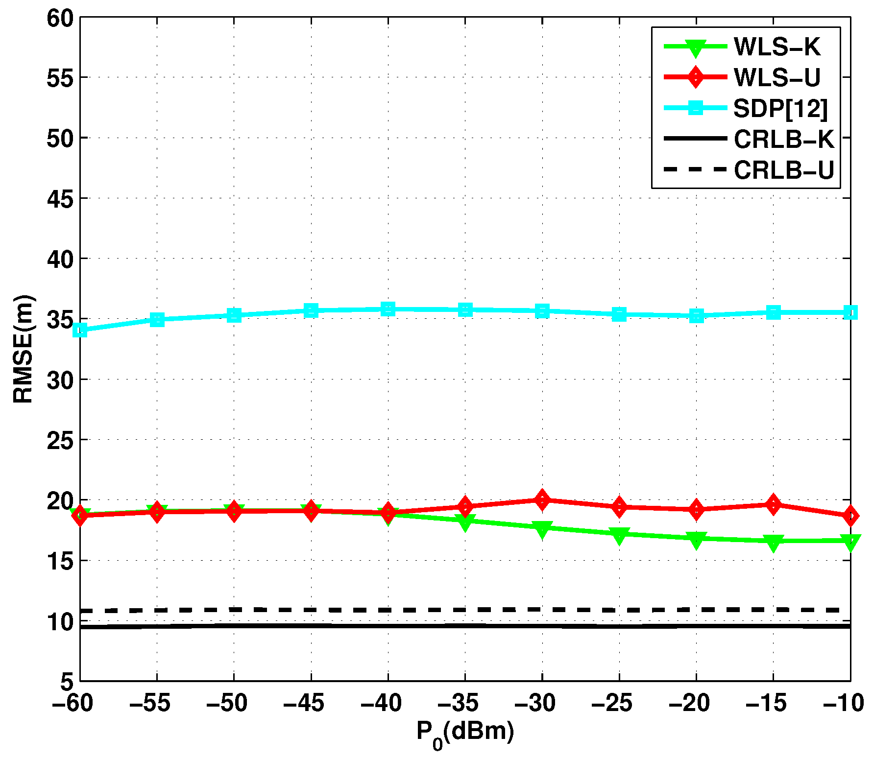
Figure 8 illustrates the RMSE versus transmit power . The figure shows that the RMSE of the discussed methods maintains a robust performance with the change in transmit power. Moreover, like the WLS-K method, the proposed WLS-U method also shows a superior performance for from to dBm.
7. Conclusions
In this paper, the target localization problems using RSS measurements in UWSN in both known and unknown transmit power cases are investigated. Firstly, an optimization problem for estimating target localization in both cases is presented. The derived objective function is then transformed into a GTRS framework. Efficient implementation methods are provided in both known and unknown target transmit power cases. The closed-form expressions of the CRLBs in both cases are derived. Computer simulation results confirm the effectiveness of the proposed methods in underwater acoustic environments.
8. Further Research
This study was limited to a stationary environment where the anchor and target node positions are unchanged during the observation period. In most UWSN environments, however, the positions of the target or anchor nodes change. Therefore, the localization method for mobile nodes in UWSN should be studied.
Acknowledgments
The authors gratefully acknowledge the grants from the National Natural Science Foundation of China (61571250), the Ningbo Natural Science Foundation(2015A610121), the Public Welfare Technology Application Research Project of Zhejiang Province of China (2016C31095), and the K.C. Wong Magna Fund of Ningbo University.
Author Contributions
Shengming Chang and Youming Li conceived and designed the entire procedure described in this paper and finished the CRLB analysis. Yucheng He assisted in performance comparisons between methods. Hui Wang performed the computer simulations and carried out the complexity analysis.
Conflicts of Interest
The authors declare no conflict of interest.
Abbreviations
The following abbreviations are used in this paper:
| UWSN | Underwater Acoustic Wireless Sensor Network |
| UWA | Underwater Acoustic |
| RSS | Received Signal Strength |
| ToA | Time-of-Arrival |
| TDoA | Time-Different-of-Arrival |
| AoA | Angle-of-Arrival |
| SDP | Semi-Definite Programming |
| Probability Density Function | |
| ML | Maximum Likelihood |
| WLS | Weighted Least Square |
| WLS-K | Weighted Least Square-Known |
| WLS-U | Weighted Least Square-Unknown |
| GTRS | Generalized Trust Region Subproblem |
| CRLBs | Cramer–Rao Lower Bounds |
| CRLB | Cramer–Rao Lower Bound |
| CRLB-K | Cramer–Rao Lower Bound-Known |
| CRLB-U | Cramer–Rao Lower Bound-Unknown |
| RMSE | Root Mean Square Error |
| Mc | Monte Carlo |
| CDF | Cumulative Density Function |
| ME | Mean Error |
Appendix A. CRLBs Deduction
Appendix A.1. CRLB Deduction in the Known Target Transmit Power Case
In the known target transmit power case, according to the observation vectors in Equation (1), the condition PDF in the given is
where , and .
Thus, the log-likelihood function w.r.t the variable has the following form
For any unbiased estimator, i.e., , the covariance matrix is lower bound by , where is the Fisher information matrix (FIM). The CRLB is the inverse of FIM, , which can be derived from Equation (A2) as follows:
Therefore,
Based on the assumption that is a zero mean Gaussian random variable with the covariance matrix , and taking the negative expectation on both sides of Equation (A4), we have
where with
Finally, we derive the closed-form expression of the CRLB in the known target transmit power case as
where .
Appendix A.2. CRLB Deduction in the Unknown Target Transmit Power Case
According to the observation vectors given in Equation (1), the condition PDF of can be expressed as
where , and , .
Finally, we provide the closed-form expression of the CRLB in the unknown target transmit power case as
where .
References
- Akyildiz, I.F.; Su, W.; Sankarasubramaniam, Y.; Cayirci, E. Wireless sensor networks: A survey. Comput. Netw. 2002, 38, 393–422. [Google Scholar] [CrossRef]
- Garcia, M.; Sendra, S.; Atenas, M.; Lloret, J. Underwater wireless ad-hoc networks: A survey. In Mobile Ad Hoc Networks: Current Status and Future Trends; CRC Press: Boca Raton, FL, USA, 2011; pp. 379–411. [Google Scholar]
- Jaime, L. Underwater Sensor Nodes and Networks. Sensors 2013, 13, 11782–11796. [Google Scholar] [CrossRef]
- Tan, H.P.; Diamant, R.; Seah, W.K.G.; Waldmeyer, M. A survey of techniques and challenges in underwater localization. Ocean Eng. 2011, 38, 1663–1676. [Google Scholar] [CrossRef]
- Park, C.H.; Chang, J.H. Closed-form Two-step WLS-based TOA Source Localization Using Invariance Property of ML Estimator in Multiple-Sample Environment. IET Commun. 2016, 10, 1206–1213. [Google Scholar] [CrossRef]
- Kim, S.; Cho, J.; Park, D. Moving-target position estimation using GPU-based particle filter for iot sensing applications. Appl. Sci. 2017, 7, 1152–1166. [Google Scholar] [CrossRef]
- Rehan, K.; Qiao, G. A Survey of Underwater Acoustic Communication and Networking Techniques. Res. J. Appl. Sci. Eng. Technol. 2013, 5, 778–789. [Google Scholar]
- Fang, X.; Nan, L.; Jiang, Z.; Chen, L. Multi-channel Fingerprint Localization Algorithm for Wireless Sensor Network in Multipath Environment. IET Commun. 2017, 11, 2253–2260. [Google Scholar] [CrossRef]
- Hosseini, M.; Chizari, H.; Chai, K.S.; Budiarto, R. RSS-based distance measurement in Underwater Acoustic Sensor Networks: An application of the Lambert W function. In Proceedings of the International Conference on Signal Processing and Communication Systems, Gold Coast, Australia, 13–15 December 2011; pp. 1–4. [Google Scholar] [CrossRef]
- Kim, C.; Lee, S.; Kim, K. 3D underwater localization with hybrid ranging method for near-sea marine monitoring. In Proceedings of the International Conference Embedded and Ubiquitous Computing (EUC), Melbourne, Australia, 24–26 October 2011; pp. 438–441. [Google Scholar] [CrossRef]
- Yan, Y.; Wang, W.; Shen, X.; Yang, F.; Chen, Z. Efficient convex optimization method for underwater passive source localization based on RSS with WSN. In Proceedings of the International Conference Signal Processing, Communication and Computing (ICSPCC), Hong Kong, China, 12–15 August 2012; pp. 171–174. [Google Scholar] [CrossRef]
- Xu, T.; Hu, Y.; Zhang, B.; Leus, G. RSS-Based Sensor Localization in Underwater Acoustic Sensor Networks. In Proceedings of the IEEE International Conference on Acoustics, Speech and Signal Processing (ICASSP), Shanghai, China, 20–25 March 2016; pp. 3906–3910. [Google Scholar] [CrossRef]
- Wang, B.; Li, Y.; Huang, H.; Zhang, C. Target Localization in Underwater Acoustic Sensor Networks. In Proceedings of the Congress on Image and Signal Process, Sanya, China, 27–30 May 2008; Volume 4, pp. 68–72. [Google Scholar] [CrossRef]
- More, J.J. Generalization of the Trust Region Problem. Optim. Methods Soft 1993, 2, 189–209. [Google Scholar] [CrossRef]
- Tomic, S.; Beko, M.; Dinis, R. 3-D Target Localization in Wireless Sensor Network Using RSS and AoA Measurements. IEEE Trans. Veh. Technol. 2016, 66, 3197–3210. [Google Scholar] [CrossRef]
- Brekhovskikh, L.M.; Lysanov, Y.P. Fundamentals of ocean acoustics (3rd edition). J. Acoust. Soc. Am. 2004, 116, 1863. [Google Scholar] [CrossRef]
- Vaghefi, R.M.; Buehrer, R.M. Received Signal Strength-based Sensor Localization in Spatially Correlated Shadowing. In Proceedings of the IEEE International Conference on Acoustics, Speech and Signal Processing (ICASSP 2013), Vancouver, BC, Canada, 26–31 May 2013; pp. 4076–4080. [Google Scholar] [CrossRef]
- Qarabaqi, P.; Stojanovic, M. Statistical characterization and computationally efficient modeling of a class of underwater acoustic communication channels. IEEE J. Ocean. Eng. 2013, 38, 701–717. [Google Scholar] [CrossRef]
- Beck, A.; Stoica, P.; Li, J. Exact and approximate solutions of source localization problems. IEEE Trans. Signal Process. 2008, 56, 1770–1778. [Google Scholar] [CrossRef]
- Stojanovic, M. On the relationship between capacity and distance in an underwater acoustic communication channel. In Proceedings of the 1st ACM International Workshop on Underwater Networks, Los Angeles, CA, USA, 25 September 2006; ACM: New York, NY, USA, 2007; Volume 11, pp. 34–43. [Google Scholar] [CrossRef]
- Stojanovic, M.; Preisig, J. Underwater acoustic communication channels: Propagation models and statistical characterization. IEEE Commun. Mag. 2009, 47, 84–89. [Google Scholar] [CrossRef]
- Cui, J.H.; Kong, J.; Gerla, M.; Zhou, S. The challenges of building mobile underwater wireless networks for aquatic applications. IEEE Netw. 2006, 20, 12–18. [Google Scholar] [CrossRef]
- Pólik, I.; Terlaky, T. Interior Point Methods for Nonlinear Optimization. In Nonlinear Optimization, 1st ed.; Di Pillo, G., Schoen, F., Eds.; Springer: Berlin, Germany, 2010; Chapter 4; Volume 1989, pp. 215–276. [Google Scholar] [CrossRef]
- Grant, M.; Boyd, S. CVX: Matlab Software for Disciplined Convex Programming. version 2.1. Available online: http://cvxr.com/cvx (accessed on 15 September 2014).
- Sturm, J.F. Using SeDuMi 1.02, a MATLAB Toolbox for Optimization Over Symmetric Cones. Opt. Methods Soft 1999, 11, 625–653. [Google Scholar] [CrossRef]
Figure 1.
The i-th sensoring link in the underwater acoustic wireless sensor network (UWSN) model.
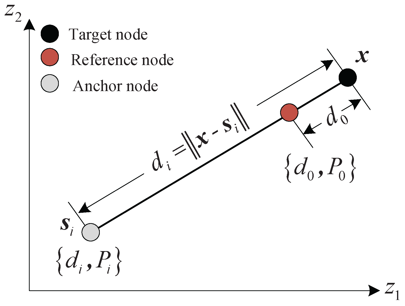
Figure 2.
Absorption coefficient, , versus frequency.

Figure 3.
versus the transmit power in Equation (18) for several .
Figure 3.
versus the transmit power in Equation (18) for several .
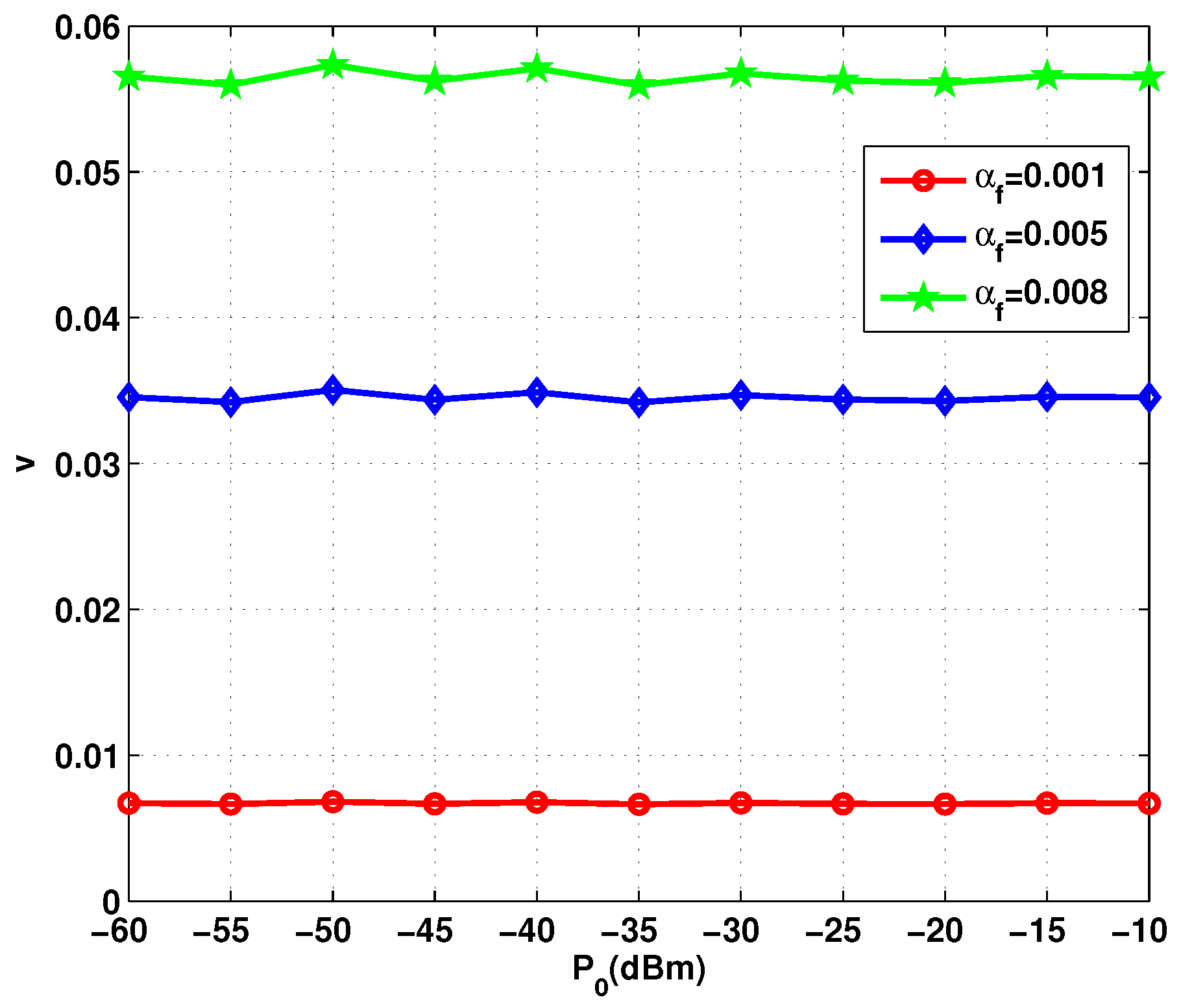
Figure 4.
Root mean square error (RMSE) versus the when N = 10, = 0.001 dB/m (f = 9 kHz), and = 0.8.
Figure 4.
Root mean square error (RMSE) versus the when N = 10, = 0.001 dB/m (f = 9 kHz), and = 0.8.
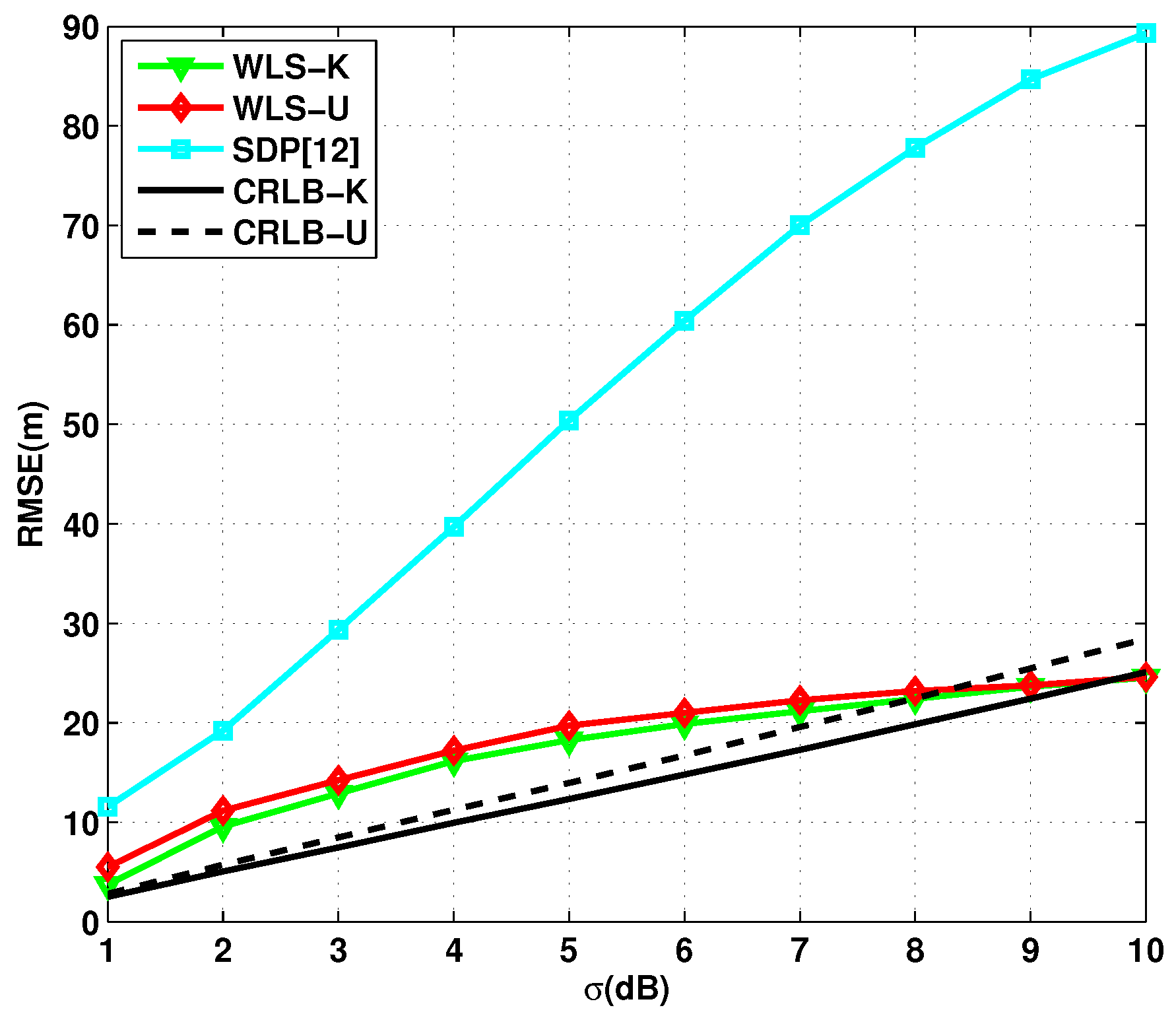
Figure 5.
RMSE versus the anchor node number N when = 4 dB, = 0.01 dB/m (f = 34 kHz), and = 0.8.

Figure 6.
Cumulative density function (CDF) versus mean error (ME) when = 4 dB, = 0.1 dB/m (f = 454 kHz), N = 10, and = 0.8.
Figure 6.
Cumulative density function (CDF) versus mean error (ME) when = 4 dB, = 0.1 dB/m (f = 454 kHz), N = 10, and = 0.8.
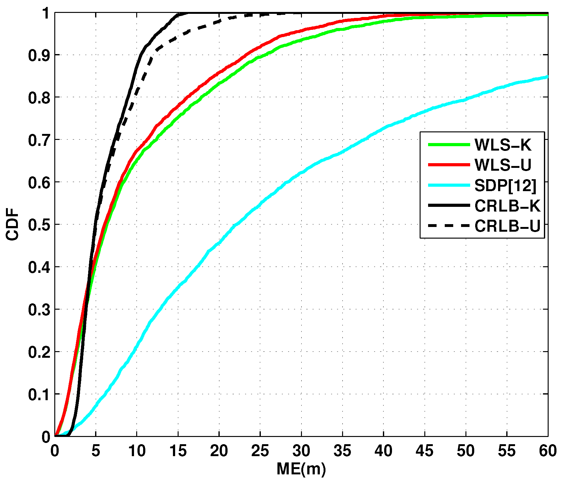
Figure 7.
RMSE versus absorption coefficient when = 4 dB, N = 10, and = 0.8.

Figure 8.
RMSE versus transmit power when = 4 dB, = 0.01 dB/m (f = 34 kHz), N = 10, and = 0.8.

© 2018 by the authors. Licensee MDPI, Basel, Switzerland. This article is an open access article distributed under the terms and conditions of the Creative Commons Attribution (CC BY) license (http://creativecommons.org/licenses/by/4.0/).
Share and Cite
MDPI and ACS Style
Chang, S.; Li, Y.; He, Y.; Wang, H. Target Localization in Underwater Acoustic Sensor Networks Using RSS Measurements. Appl. Sci. 2018, 8, 225. https://doi.org/10.3390/app8020225
AMA Style
Chang S, Li Y, He Y, Wang H. Target Localization in Underwater Acoustic Sensor Networks Using RSS Measurements. Applied Sciences. 2018; 8(2):225. https://doi.org/10.3390/app8020225
Chicago/Turabian StyleChang, Shengming, Youming Li, Yucheng He, and Hui Wang. 2018. "Target Localization in Underwater Acoustic Sensor Networks Using RSS Measurements" Applied Sciences 8, no. 2: 225. https://doi.org/10.3390/app8020225
Note that from the first issue of 2016, this journal uses article numbers instead of page numbers. See further details here.