Cloud Incubator Car: A Reliable Platform for Autonomous Driving


División de Sistemas en Ingeniería Electrónica (DSIE), Universidad Politécnica de Cartagena, Campus Muralla del Mar, s/n, 30202 Cartagena, Spain
*
Author to whom correspondence should be addressed.
†
These authors contributed equally to this work.
Appl. Sci. 2018, 8(2), 303; https://doi.org/10.3390/app8020303
Submission received: 30 November 2017
/
Revised: 5 February 2018
/
Accepted: 11 February 2018
/
Published: 20 February 2018
(This article belongs to the Special Issue Road Vehicles Surroundings Supervision: On-Board Sensors and Communications)
Abstract
:It appears clear that the future of road transport is going through enormous changes (intelligent transport systems), the main one being the Intelligent Vehicle (IV). Automated driving requires a huge research effort in multiple technological areas: sensing, control, and driving algorithms. We present a comprehensible and reliable platform for autonomous driving technology development as well as for testing purposes, developed in the Intelligent Vehicles Lab at the Technical University of Cartagena. We propose an open and modular architecture capable of easily integrating a wide variety of sensors and actuators which can be used for testing algorithms and control strategies. As a proof of concept, this paper presents a reliable and complete navigation application for a commercial vehicle (Renault Twizy). It comprises a complete perception system (2D LIDAR, 3D HD LIDAR, ToF cameras, Real-Time Kinematic (RTK) unit, Inertial Measurement Unit (IMU)), an automation of the driving elements of the vehicle (throttle, steering, brakes, and gearbox), a control system, and a decision-making system. Furthermore, two flexible and reliable algorithms are presented for carrying out global and local route planning on board autonomous vehicles.
1. Introduction
It appears clear that the road transport will be going through enormous changes in the near future (intelligent transport systems), although, presumably, gradual, in which new technologies will have a prevailing role [1]. Thus, in the Horizon 2020 EU work program, smart, green, and integrated transport are placed as the main pillars for transport in the future. Among the program lines the following can be distinguished: “Safe and connected automation in road transport, where specific requirements are imposed on simple automation, limiting its foreseeable scope in the short term.” Without a doubt the most disruptive technological challenge is focused on the so called autonomous vehicle and, the next step, autonomous cooperative vehicles [2]. However, some issues need to be addressed: (1) the operation must be completely reliable and safe [3]: this specification is a highly demanding requirement, which usually complies with limiting the application of these vehicles to controlled scenarios, simple applications, or at reduced speeds of operation. Thus, it is understood that autonomous driving is viable in dedicated lanes or areas in situations of congestion or in parking manoeuvres, which is already a reality in many cases. Collision avoidance safety systems are more complex, especially those that take control of the vehicle in emergency manoeuvres; (2) the cost of sensors and control hardware must comply with what the market can assume, so that the mass production of vehicles can be economically affordable [4]; (3) much work is still necessary concerning legal and social issues, i.e., the question of liability where an automated vehicle is involved in an accident causing property damage or personal injury [5].
Regarding the above, it can be said that fully automated driving is not a technological utopia, but its practical implementation on the roads should be carefully analysed [6]. Researchers and manufacturers advocate for automation in successive stages, firstly approaching longitudinal control, then simple side controls, to reach complete automation in scenarios of increasing complexity. In a few words, the change from conventional to assisted driving is now a reality, and the leap is being made towards automated driving in its different stages: partial, high, or fully automated.
Intelligent vehicles (IV) are one of the key elements within intelligent transport systems. When an IV has intelligence—understood as the fact that the control relies on the onboard vehicle processing systems, it can move autonomously. The onboard vehicle intelligence becomes aware of the situation of the vehicle in its environment and performs all the necessary control actions to proceed towards its destination.
Driving automation—considered a low-risk activity for humans—is a matter that needs the continuous evaluation of two main factors: (a) the current vehicle state (position, velocity, acceleration, direction) and (b) the environmental conditions (nearby vehicles, obstacles, pedestrians, etc.). To the extent that these two factors are accurately assessed, appropriate decisions can be taken towards reliable autonomous driving, and we will be closer to a vehicle-centric [6] approach to autonomous driving, where the main goal is the safe movement of the vehicle.
It is not an easy task to define what an IV with autonomous abilities is, although it is possible to describe its capacities, as detailed in Table 1 [7].
But, what exactly does autonomous driving mean? Following the policy defined by the NHTSA (National Highway Traffic Safety Administration, USA) [8], the International Society of Automotive Engineers (SAE) has set three categories of advanced driving automation, which imply the automation of both the driving actions (steering, throttle, and break) and the monitoring of the driving environment (see Table 2) [9].
Platforms for Autonomous Driving Development
The mass production of autonomous vehicles still has to wait because of different concerns, such as reliability, safety, cost, appearance, and social acceptance, to say just a few [10]. Advances in the state-of-the-art of sensing and control software have allowed great improvements in the reliability and safe operation of autonomous vehicles in real-world conditions, in part thanks to a great variety of development platforms [7,11,12,13]. Table 3 shows the main features of some of the prominent ones.
The latest approach to autonomous driving is the so-called cloud-based autonomous driving [14,15]. These clouds provide essential services to support autonomous vehicles. Currently, these services include simulation tests for new algorithm deployment, offline deep learning model training, and High-Definition (HD) map generation. Autonomous driving clouds have infrastructures that include distributed computing, distributed storage, as well as heterogeneous computing. When driving algorithms and strategies are ready, they must be implemented in real control systems for adjusting and testing purposes before getting the car into real traffic conditions. Reliable control systems will be very useful for this purpose. This implies the interest of having a hardware–software development platform for control purposes that can be easily adapted to any car, thus allowing the autonomous driving system developers to concentrate exclusively on the sensory and algorithmic aspects of the prototypes. On the other hand, it is interesting to continue integrating new sensing techniques that allow a better and faster characterization of the environment, thus making possible to develop driving algorithms with a more precise behaviour.
The rest of the manuscript has been divided into three sections. Section 2 details the mechanical, electrical, and electronics modifications carried out to create the CICar platform. Section 3 shows the three components of high-level architecture proposed: a control system, a perception system, and a decision-making system. Furthermore, two novel algorithms are presented and used by the decision-making system for global and local path planning. Finally, Section 4 presents our conclusions.
2. Cloud Incubator Car Platform
As described above, autonomous driving technologies are making the transition from laboratories to the real world, and so must the vehicle platforms used to test and develop them. Research teams develop their own experimental platforms and also develop proprietary control systems.
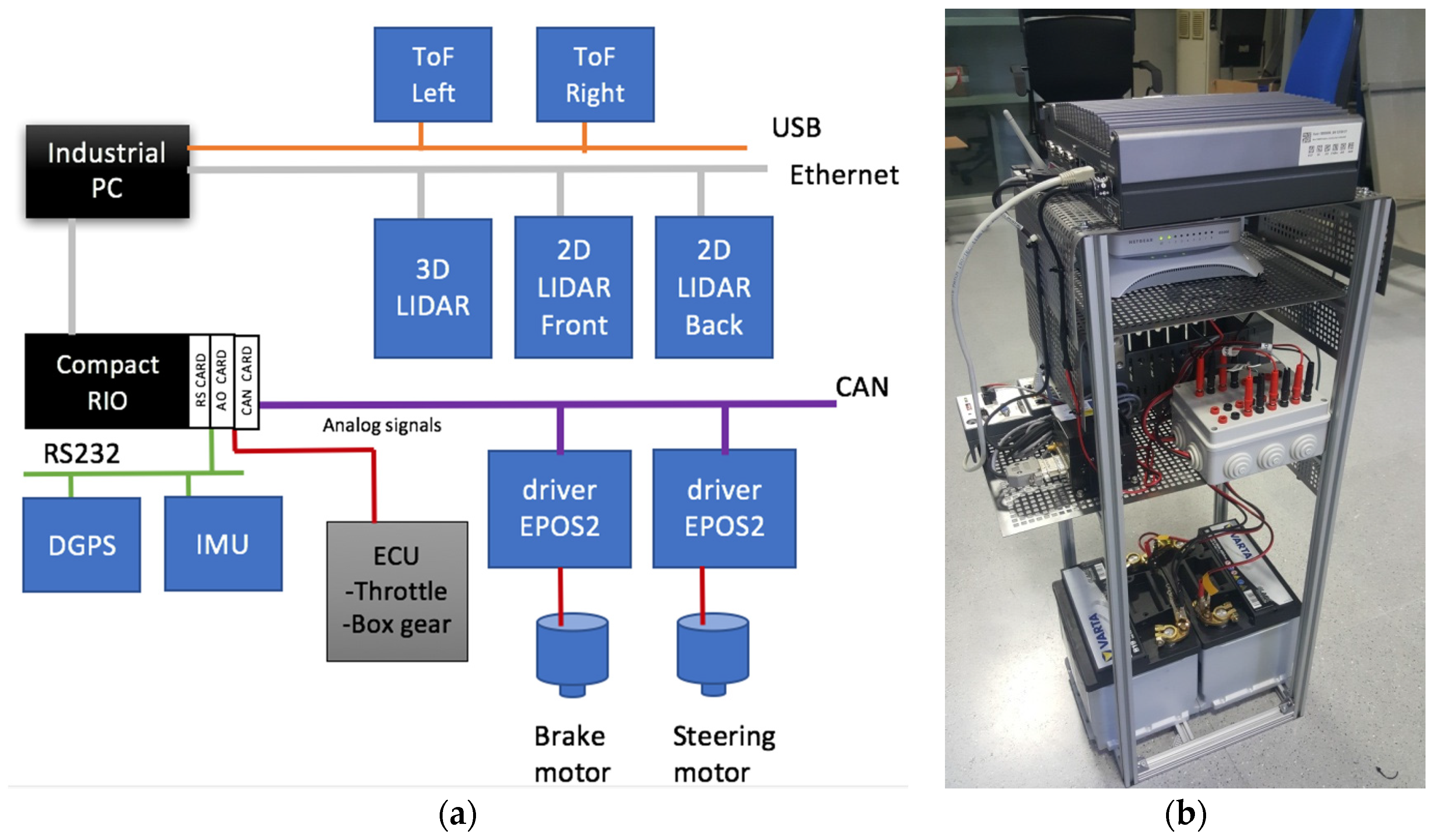
In the Intelligent Vehicles Lab at the Technical University of Cartagena we have developed a comprehensible and reliable platform for autonomous driving technology development as well as for testing purposes: the CICar (Cloud Incubator Car, Figure 1a). This platform allows a complete experimentation of the aspects related to the integration of third-party sensors (laser range finders, global positioning systems, vision cameras, etc.), control of devices (motors, actuators, etc.), and industrial buses for communication. Software development has been made a comprehensible task by using a well-known hardware–software development platform for control purposes: RIO architecture and LabVIEW [16].
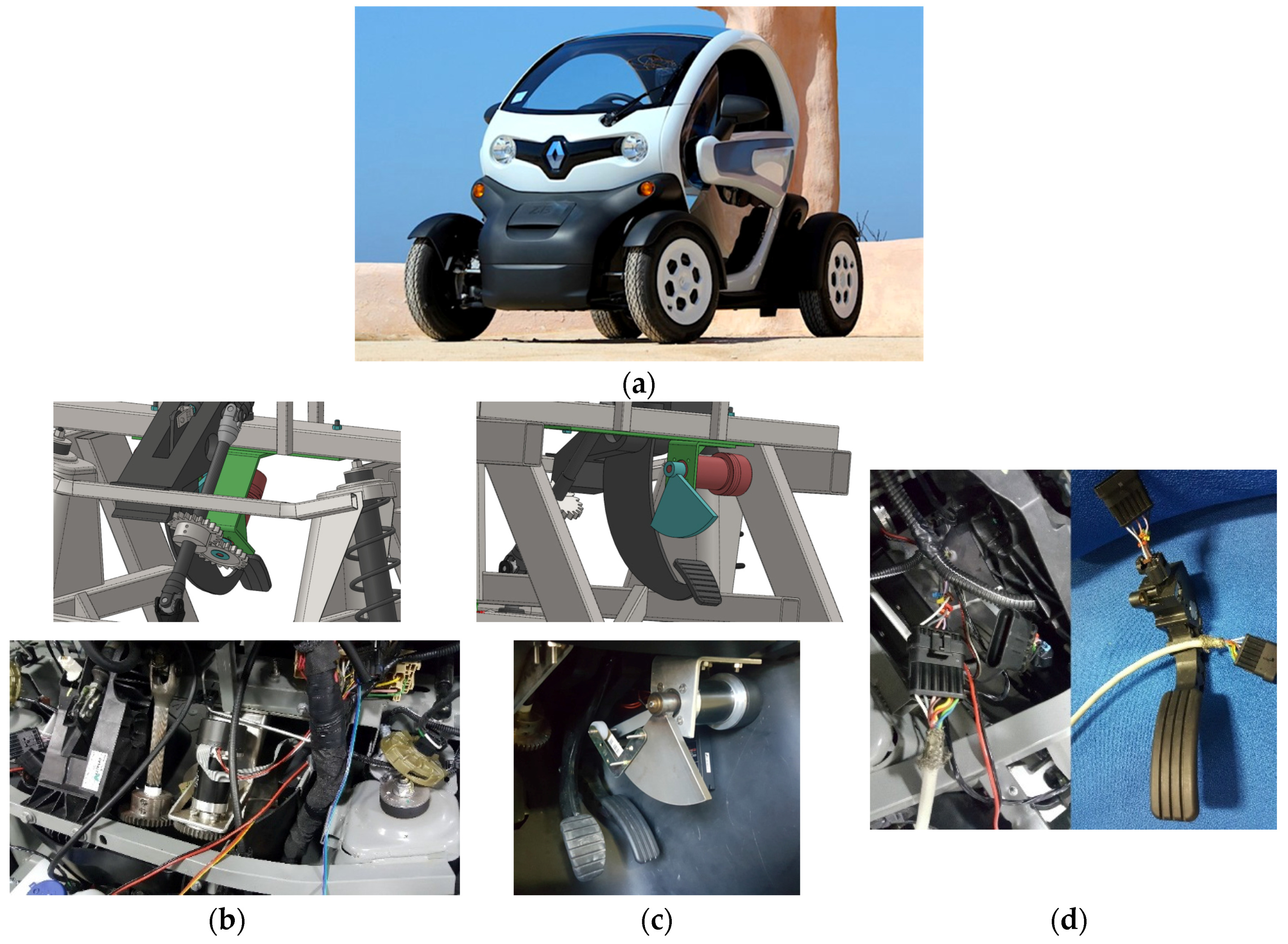
The aforementioned platform is based on an electric commercial vehicle—Renault Twizy—that has been conveniently modified in order to meet the specifications mentioned above. The modifications compound the low label architecture and include: (a) automation of driving elements (throttle, brake, steering, gearbox); (b) installation of external anchors capable of holding a wide variety of sensors; (c) installation of interior racks to accommodate the different control and processing systems (Figure 2b); (d) installation of electrical facilities and communication buses to feed and connect the different sensors and the control and processing hardware.
2.1. Modification of the Steering System
The modification of the steering system is a basic mechanical solution, as shown in Figure 1b, which consists of acting on the steering column or axis. A mechanical gear motor assembly is fixed to the steering column with gears, allowing the axis to turn. The original axis has not been modified, and this allows both steering control modes: automatic and manual. The mechanical implementation of the steering automation complies with the requirements of angular position range and precision, in addition to those of axis movement maximum speed (60 rpm). The steering system actuator is composed of an electronic driver EPOS2 and a motor from MAXON (EC60fl-GP52C-1024IMP-100W from Maxon Motor, Sachseln, Switzerland, acquired in Spain delegation).
2.2. Modification of the Braking System
The modification of the braking system, in the same way as that of the steering system, is not invasive of the original system. It has been implemented using a mechanical assembly with a motor comprising a gear coupled to a cam that presses the brake pedal by means of a short displacement of about 15° with force control (see Figure 1c). The braking system actuator is composed of an electronic driver EPOS2 and a motor from MAXON (EC60fl-GP52C-1024IMP-100W from Maxon Motor, Sachseln, Switzerland, acquired in Spain delegation).
2.3. Throttle and Gearbox Modifications
We have devised an electronic solution for the throttle and gearbox automation. After scanning the control signals, it is possible that the electronic device, which is attached to the throttle pedal, exchanges data with the vehicle’s ECU (Electronic Control Unit). In the same way, it is possible to select PDNR (P=Park, D=Driver, N=Neutral, R=Reverse) in the gearbox by means of the control system. We have developed a software module which emulates its operation through an analogue card. It works in parallel with the original system, so both manual and automatic throttle control are offered (see Figure 1d).
2.4. Sensor Holders
We have installed on the CICar vehicle a varied set of supports capable of holding different types of sensors (cameras VIS, Time of Flight cameras, LIDAR 2D and 3D, IMU, GPS, etc.). For this, quick coupling devices have been used together with electrical connectors and secure communications.
2.5. Electrical and Communications Infrastructure
New electrical facilities have been installed that allow the electrical supply of both the sensors and the control and processing systems. The communication infrastructure is composed of:
- (1)
- A serial Controller Area Network (CAN bus), because of its suitability for high-speed applications using short messages, its robustness, and reliability [17].
- (2)
- (3)
- A point-to-point set communications, such as RS232 and USB.
Figure 2a shows all the components which compound the low-level architecture.
3. High-Level CICar Architecture
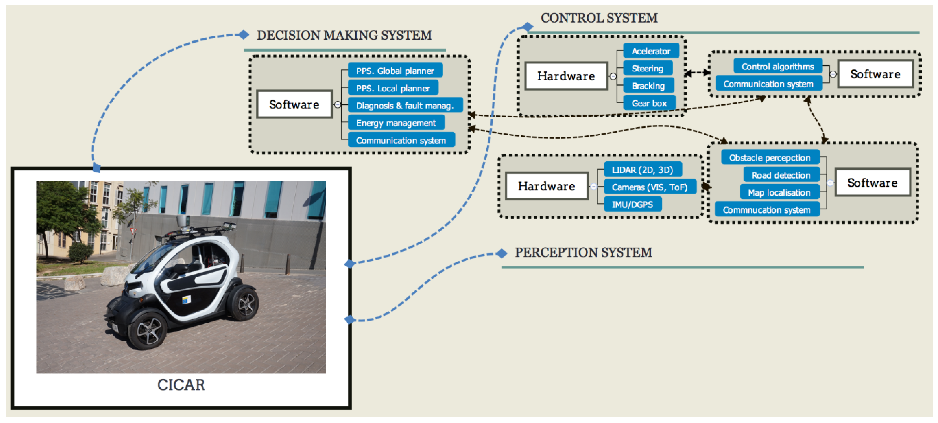
From a higher abstraction layer point of view, the architecture of the CICar is divided into: (1) a control system, (2) a perception system, and (3) a decision-making system. Figure 3 shows the distribution of the high-level architecture components of the CICar.
3.1. Control System
The goal of the control system is to translate the actions generated by the decision-making system into actuations of the elements which govern the vehicle. The control system has been implemented with a compactRIO 9082 (from National Instruments). The compactRIO processing unit is composed of two processors: an INTEL i7 and a Xilinx FPGA, which confer high performance capacities and flexibility for the testing and implementation of algorithms in the control system. The compactRIO allows soft and hard real-time processes to be run. The INTEL processor allows less critical processes to be executed, while FPGA allows time-critical processes to be executed with higher clock frequencies. The control system is governed by a Real-Time Operating System (VxWorks from WindRiver). The kernel of the CICar is designed with Finite State Machines implemented in C++ through the QS framework [20].
3.2. Perception System
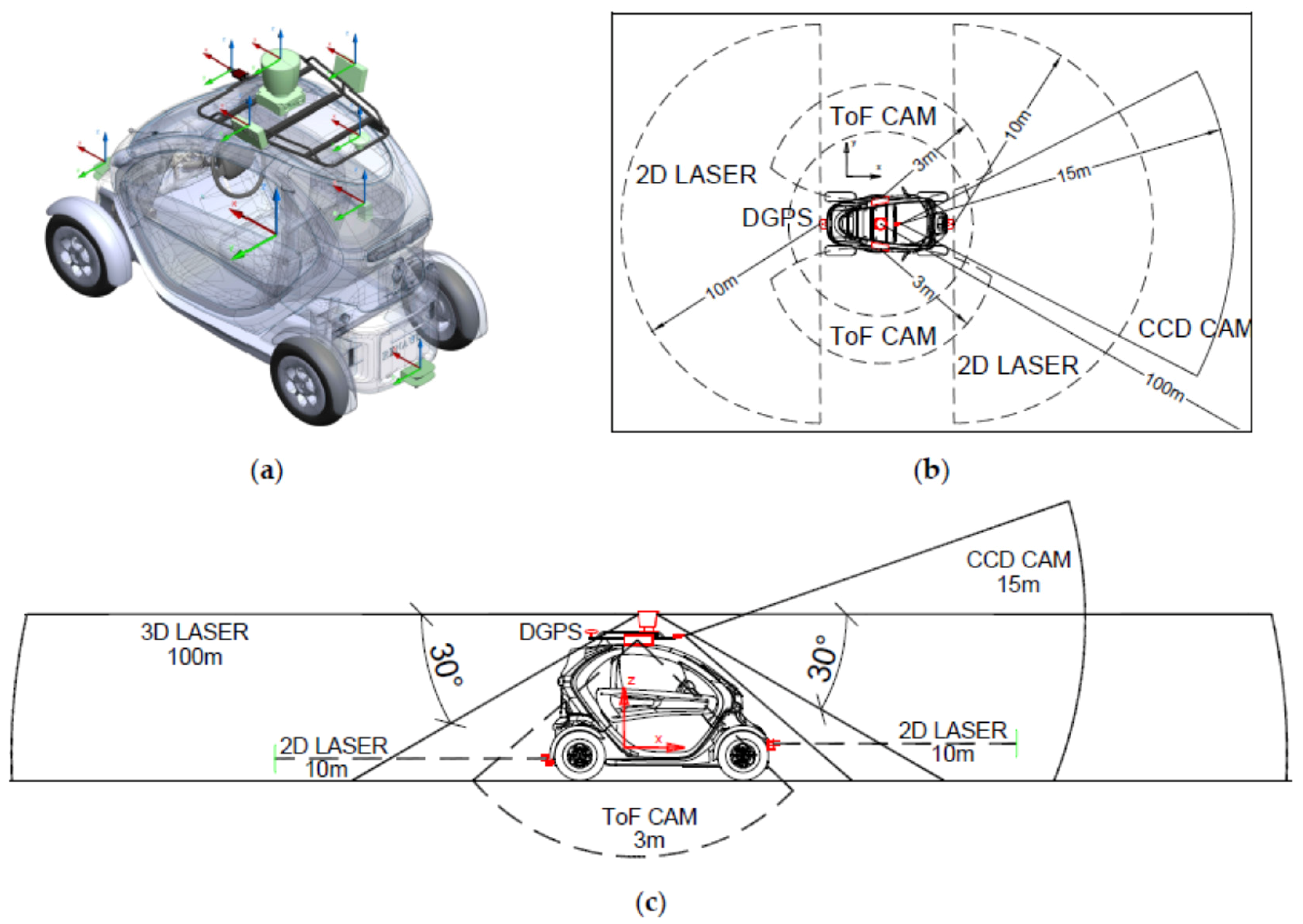
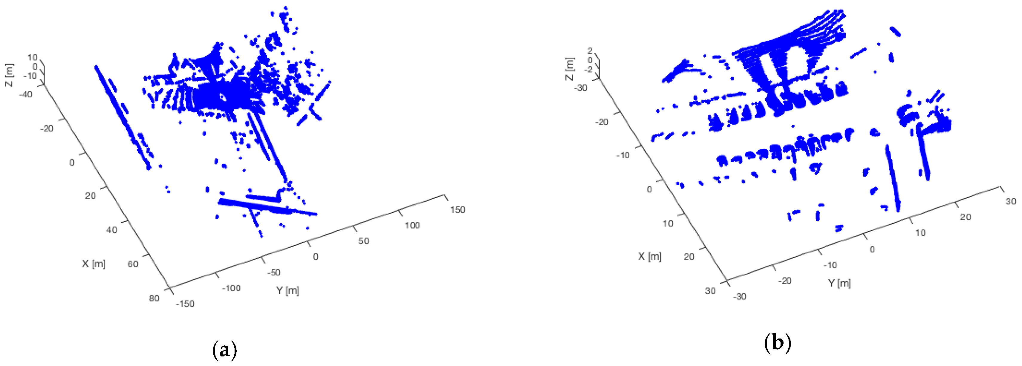
The perception system is divided into two subsystems: short- (SRS) and long-range (LRS). The perception system forms two concentric rings overlapping around the vehicle (Figure 4). The SRS allows objects to be detected up to 10 m from the front and the rear of the vehicle (2D LIDARs) and around 3 m from the right and left side of the vehicle (ToF cameras). ToF cameras are a seldom used technology in autonomous vehicles but they result to be a very attractive solution for the vehicle for short-range detection. ToFs allow 3D object detection with a high frame rate, are less affected by light conditions and shadows, and have an acceptable cost [21,22]. The objects that enter into the short-range ring suppose an inherent risk and danger for the actions of the CICar. For this reason, the sensors involved in the SRS are commanded by the RT processing unit. On the other hand, the LRS perception is based on a 3D High-Definition LIDAR (HDL64SE from Velodyne) [19]. Its 64 laser beams turn at 800 rpm and can detect objects up to 100 m away with an accuracy of 2 cm. The 3D LIDAR allows trajectories to be established (lane change, obstacle avoidance, speed reduction depending on the traffic conditions, etc.), object tracking, object classification, and behaviour prediction of other drivers. The information from the two subsystems is fused and processed to detect obstacles such as: cars, bikes, pedestrians, traffic lights, and so on. A colour camera is placed on the roof of the vehicle and is used to detect the road, lanes, road lines, and traffic signs.
The CICar has a localization system based on an RTK unit (Real-Time Kinematic), an IMU (Inertial Measurement Unit), and a relative position encoder installed on the wheel of the vehicle. RTK satellite navigation consists of a technique used to enhance the precision of the position data derived from satellite-based positioning systems (global navigation satellite systems, GNSS) such as GPS, GLONASS, Galileo, and BeiDou. The RTK is composed of a base station and a mobile unit (or rover) and it supplies an accuracy from 20 cm to 1 cm. The localization system cancels out the RTK positioning when the number of satellites detected is less than or equal to four or when the HDOP (Horizontal Dilution of Precision) is greater than five [23,24]. In these cases, the IMU and the positioning encoder installed on the vehicle are used for the localisation task. Table 4 presents a summary of the onboard sensors in the CICar.
3.3. Decision-Making System
To operate reliably in the real world, an autonomous vehicle must evaluate and make decisions about the consequences of its possible actions, anticipating the intentions of other traffic participants. The new Intelligent Decision-Making Systems are based on cognitive systems [25], agent systems [26], fuzzy systems [27], neural networks [28], evolutionary algorithms [29], multi-criteria [30] or rule-based methods [31]. The main element of the CICar is a Decision-Making System which incorporates a new local trajectory planner [32] based on Bezier curves [33].
Path-Planning System (PPS)
Global Planner
Global planners are a key element in autonomous navigation systems. The development of intelligent transport systems and autonomous vehicles has increased the demand for route planners that allow dynamic route generation, capable of adapting to the varying aspects of the road, such as traffic, roadworks, roads that have been cut off, or unexpected events. The initial requirements for the CICar global planner are listed below:
- (1)
- It must be able to create global routes using digital map sources
- (2)
- It should allow an easy introduction of traffic restrictions or unplanned events.
- (3)
- It should be executed in an agile manner and produce results in an acceptable time.
For the map source used for the global route planning, Google maps was selected, the reasons for this being:
- (1)
- It has an easily accessible Application Programming Interface (API) and is multiplatform.
- (2)
- The maps can be downloaded with different layers of information.
- (3)
- It allows georeferencing of the map points.
- (4)
- It is constantly updated and is available for free.
The first algorithm evaluated for global route generation was the A* Algorithm [34,35]. The following disadvantage was reported with the use of the A* algorithm: the algorithm was not capable of generating routes in a reasonable time using the 512 × 512 resolution binary maps tested. To increase the performance, the size of the binary maps was reduced by a constant factor (2, 3, or 4). The size reduction of the binary map speeded up the calculation time, but, because of the pixelisation effects, the following problems occurred: (1) the destruction of narrow roads, (2) the deterioration of main roads, and, as a result, (3) the routes generated were not smooth and were very abrupt.
As a solution to the problems reported, a new heuristic search algorithm for global route planning, called SCP (Search for Cross Points for obtaining global routes), was developed.
The SCP algorithm is based on a binary map of nxm pixels where the navigable routes are given a value of “1” and the non-navigable areas a value of “0”, and an initial point p0, a goal point pg, and an initial angle θ0 are set.
The stages performed by the SCP algorithm to obtain the global route are:
- A search direction is chosen (‘N’-North, ‘S’-South, ‘E’-East, ‘W’-West) according to the position of the angle between the positions pg and p0. Equation (1) shows how the search directions are obtained by the algorithm in function of the angle
![Applsci 08 00303 i001]()
- A clear path is chosen from p0 to the goal pg. A route is considered clear if all the points that form the line that joins p0 and pg have a value equal to ‘1’.
- 2.1
- If the path is not free:
- The SCP algorithm searches for the first pair of cross points [CPi; CPi+1] according to the search direction set as shown in Equation (1). To achieve this, the algorithm goes through the map, starting from p0 according to an angle θ1, until it finds a value equal to ‘0’. The point found is labelled as the first cross point CPi. Starting from CPi, and according to the search angle θ2, the algorithm searches for the next point with a value of ‘0’. This new point is labelled as the second cross point CPi+1. The angles θ1, θ2 are calculated according to the search direction and the following table.During the search for the cross points [CPi; CPi+1], the candidate points pi(xi, yi) are calculated by alternating the values of θ = θ1 and θ = θ2, based on Equation (2):with (xi−1, yi−1) being the previous value calculated, and d a constant that allows the CPi search to advance more quickly.
- The Euclidean distance between two consecutive cross points CPi and CPi+1 is calculated.
- If the distance is 0, the search direction is changed by evaluating the position of pg with respect to the last CPi+1 that was calculated, p0 is set to p0 = CPi+1, and the algorithm goes to step 2.
- If the distance is not equal to 0, p0 is set to p0 = CPi+1, and the algorithm goes to step 2.
- 2.1
- If there is a clear route, the algorithm finishes, and the path is composed of the points [p0,pm1,…,pmn−1;pg], with pm1,…,pmn−1 being the midpoints obtained from the pairs of points from the cross-point vector [p0,CP1,CP2,…,CPn;pg].

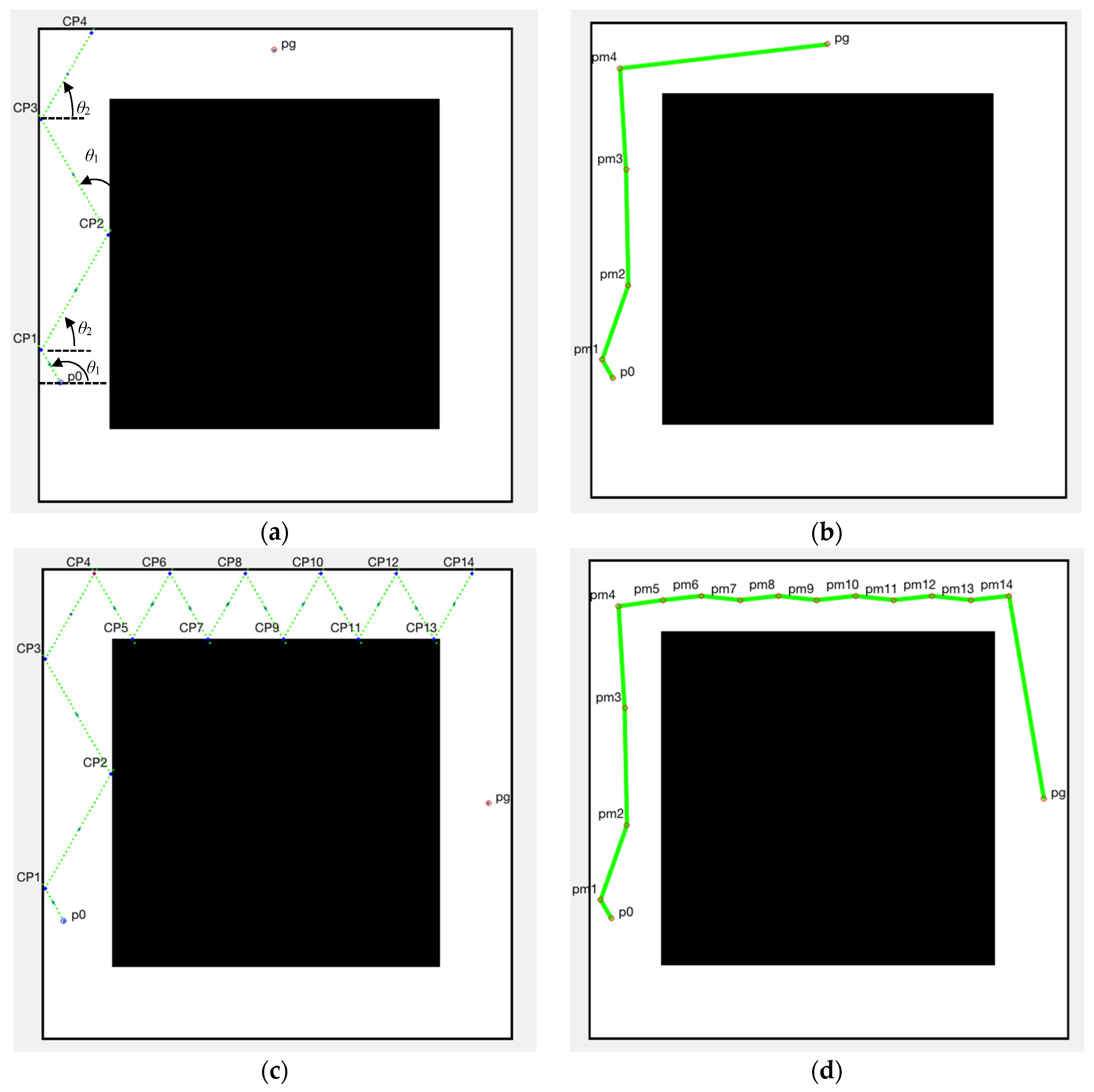
Figure 5 shows a binary map in the form of a square which will demonstrate the SCP algorithm in operation. Figure 5a shows how the SCP algorithm generates the cross points in the direction ‘N’, given the information (p0, pg, θ0). In the example with θ0 = 60° and Table 5, the angles θ1 y θ2 are −120° and −60° respectively.
As shown in Figure 5a, the cross points CPi are generated in a zigzag in the direction ‘N’ until a direct path to the destination is found. Figure 5b shows the route generated between the midpoints of the segments from the set [p0CP1; CP1CP2; CP2CP3; CP3CP4; CP4pg]. In Figure 5c, a more complex scenario with a different pg is shown. In this case, when the SCP algorithm reaches CP5, an end of route occurs when it no longer follows the ‘N’ direction. At this point, the Euclidean distance between CP4 and CP5 is 0, and the algorithm changes the search direction from ‘N’ to ‘E’, with θ1 = 60° and θ2 = −60°. With the change of direction, it is possible to calculate a new CP5. Figure 5d shows the route generated between the midpoints of the segments from the set [p0CP1,…, CP14pg].
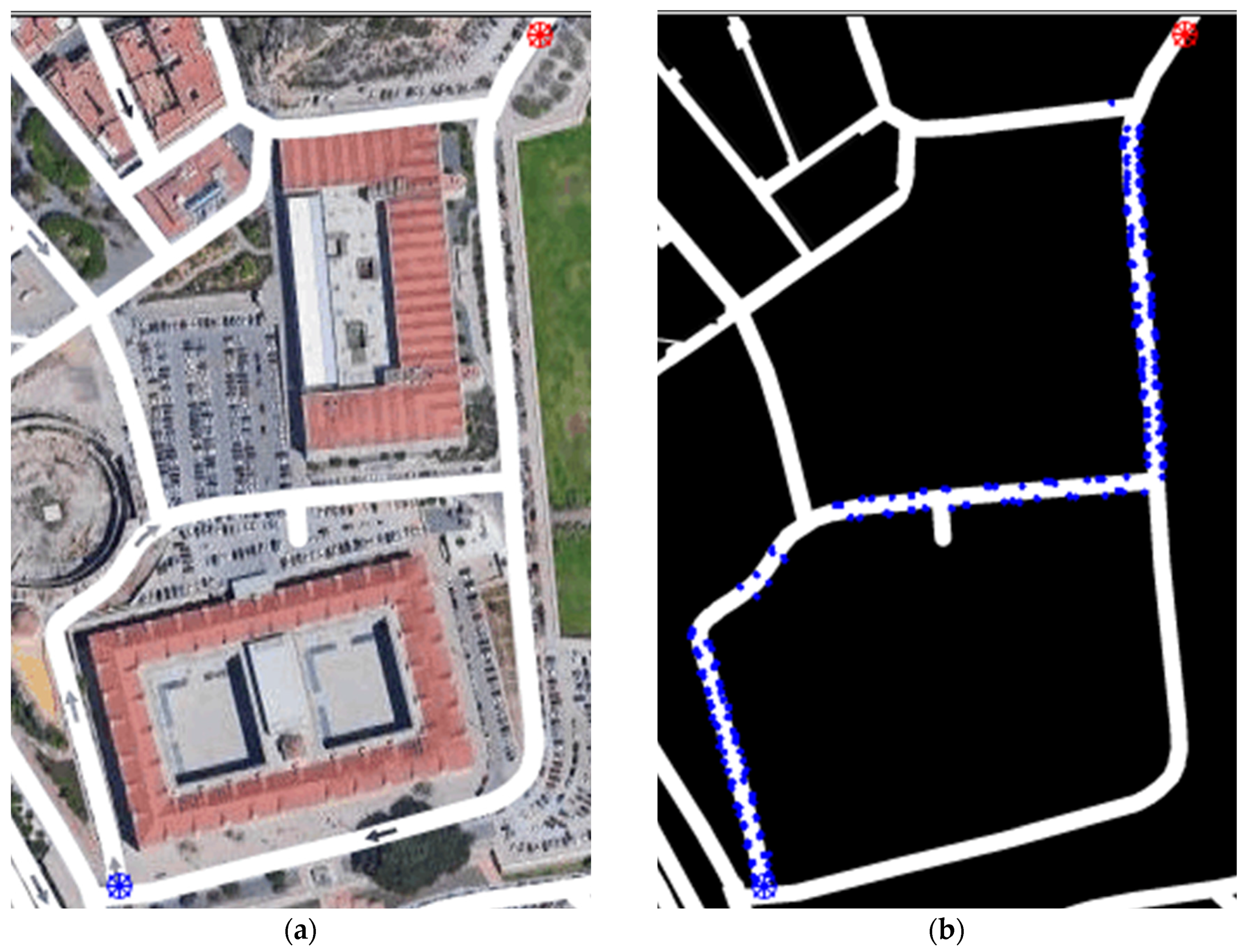
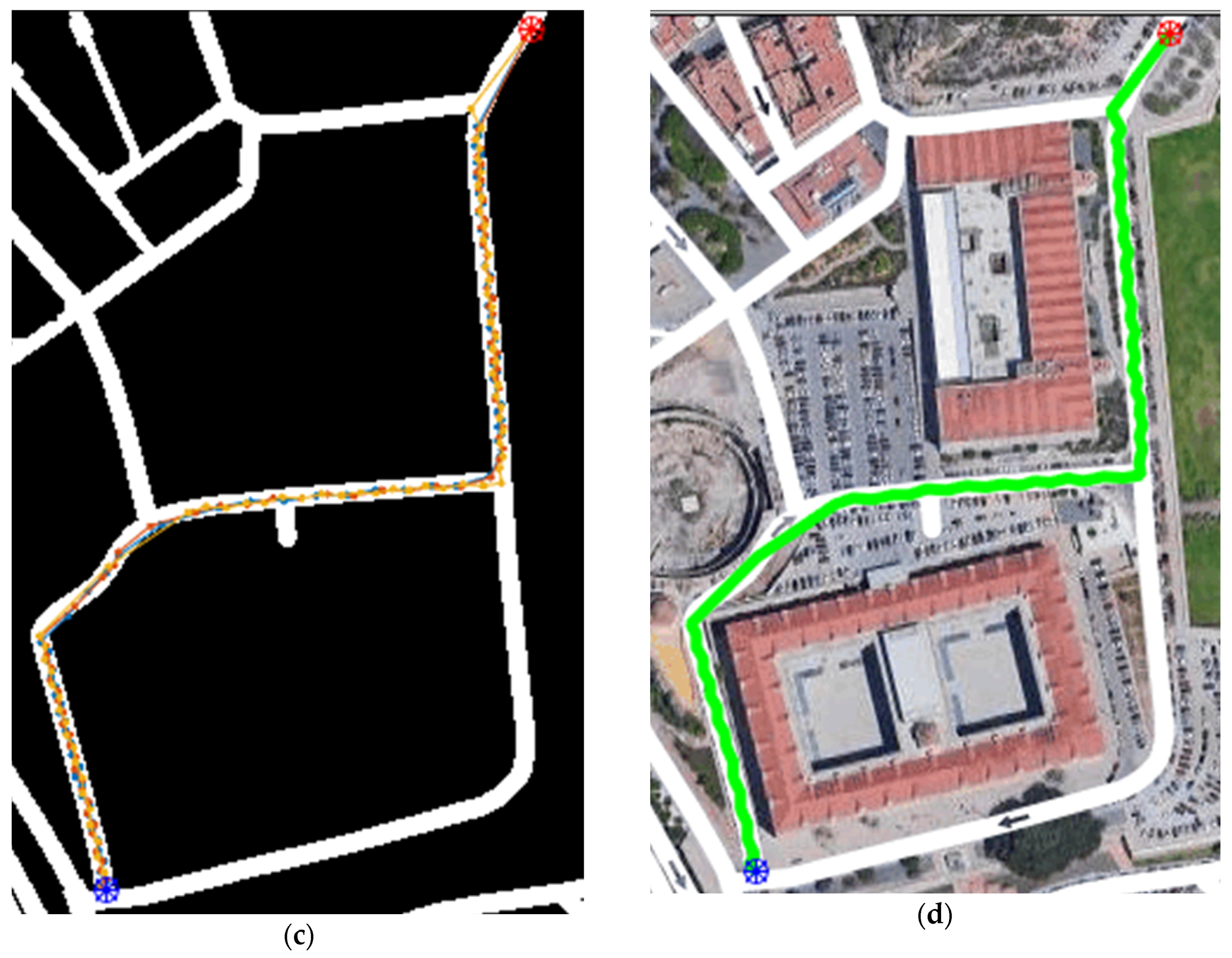
The SCP algorithm can increase the number of routes calculated with a greater number of initial starting angles. Figure 6a shows a real map of the Technical University of Cartagena where an initial point p0 and a final point pg (blue and red crosses) have been selected.
The SCP algorithm has been executed with initial angles θ0 from 20 to 80 degrees, with 2-degree increments. After its execution, the SCP has calculated three possible trajectories. Figure 6b shows the cross points found, and Figure 6c the trajectories created from the set of midpoints from the three calculated trajectories. Figure 6d shows the optimal path calculated as the shortest between points p0 and pg.
The optimal path is partitioned in waypoints (WP0,…, WPi,…, WPn). The waypoints will be used by the CICar to establish short missions between them using the local planner module. The CICar location is provided by a DGPS unit on board the vehicle.
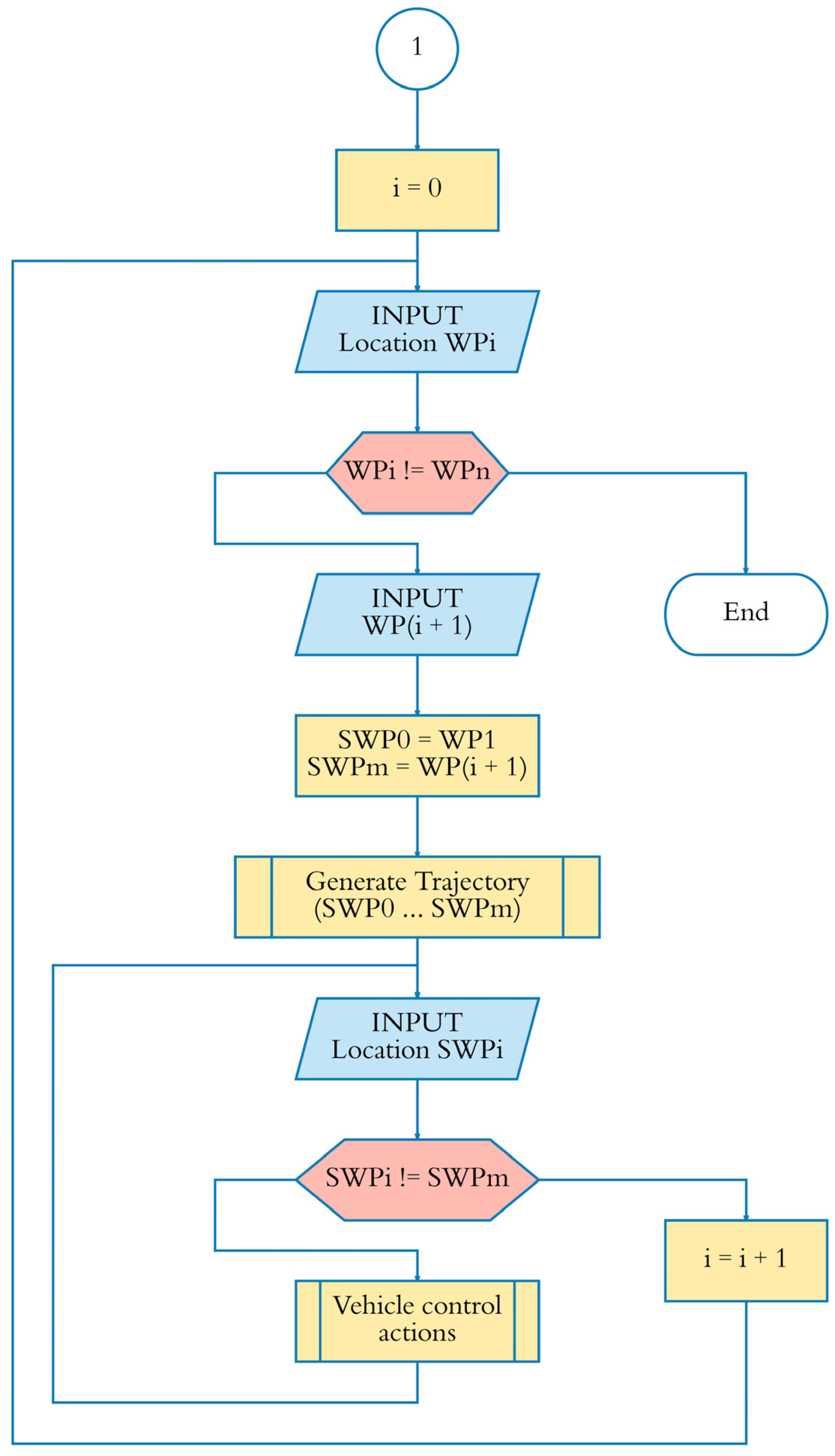
Local Planner
The local planner uses a pair of waypoints (WPi, WPi+1) supplied by the global planner to generate a set of possible trajectories to reach WPi+1 from WPi (see Figure 7).
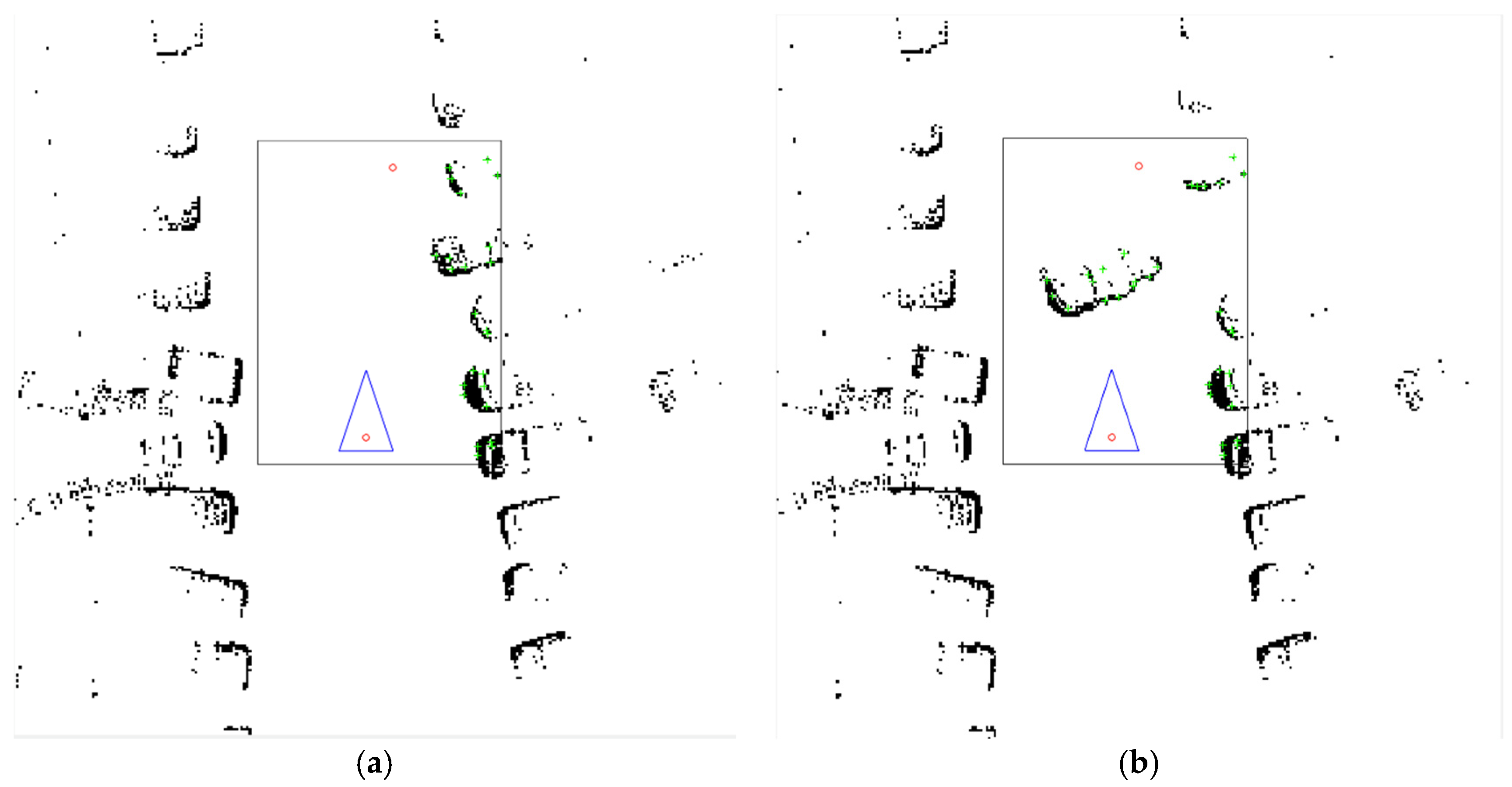
For that, the perception system supplies a local map of up to 100 m around the vehicle (Figure 8a), which is completed with three constraint types: (a) the constraints that the vehicle detects on the way by means of the perception system (vehicles, pedestrian, bikes, curbs, and so on), (b) the limitations inherent in the vehicle characteristics (wide, high, kinematic model), c) the constraints derived from the traffic rules (one way, bidirectional way, traffic signs, etc.). To decrease the number of computations and to increase the performance, the perception system supplies a set of keypoints which are a representation of the surroundings of the vehicle. The keypoint set is obtained after applying a filtering process composed of two stages:
- Distance filter. All XYZ points beyond a maximum distance (dmax) will be rejected.Distance filter. All XYZ points beyond a maximum distance (dmax) will be rejected.
- High filter. All Z points higher than a maximum value (Zmax) will be discarded.
As shown in Figure 8b, we have simplified the initial XYZ local map to obtain a compact profile of the XYZ representation of the objects in the scene.
After this, the corners of the objects in the scene are computed using the Harris algorithm [36]. The Harris algorithm is applied over an ROI (Region of Interest) in the forward direction of the vehicle. Figure 9 shows the results of corner detection in the ROI of two scenarios extracted from Figure 9b. This group of points calculated by the Harris algorithm are called keypoints (KPi) and will be used in the next stage of the PPS to create a set of trajectories.
In Figure 9, green crosses represent the keypoint set, a triangle with a 2 metre base represents the vehicle, a rectangle shows the ROI where the Harris detector is computed, and two red circles represent the origin and goal locations (WPi, WPi+1).
The trajectory generator module receives two waypoints (WPi, WPi+1) and a set of keypoints {KP0,…,KPk} representative of the environment around the vehicle for computing a set of trajectories between a pair of waypoints. The module uses the Bezier curves to generate possible trajectories between the waypoints, using the keypoints as control points.
A Bezier curve of grade n can be generalized by the Equation (3) [33]:
For example, the second-grade curve (n = 2) is (see Equation (4)):
Being P0, P1, and P2 the control points, and t a real value between 0 and 1. A higher step of t allows a higher number of points to be obtained in the Bezier curve generation B(t).
The trajectory generator module implements a set of second-grade Bezier curves displaced along the X-axis control point P1. The development algorithm is shown in Algorithm 1, where nCurves indicates the number of trajectory candidates which have been calculated. However, only one set will pass the security distance constraints and will be adopted as the trajectory (Ti[]). For each of them, a new control point P1 is defined, one half to the left of the midpoint between P0 and P2, and the other half to the right. In Figure 9, line 1.2., a control point displacement increment equal to 3.0 is defined. fB is a function that generates a second-grade Bezier curve between P0 and P2. The function fP1 searches for the Pi point with the lowest Euclidean distance to set the Bezier points of B(t).
After a set of trajectories is obtained Ti = {B(t)0,..., B(t)m}, the optimal trajectory can be established under different criteria depending on the conditions in each moment during autonomous driving. In this work, we have implemented three criteria to select the optimal trajectory: (a) the minimum distance travelled, (b) the maximum angle travelled, and (c) the medium trajectory.
| Algorithm 1 Trajectory generator algorithm. |
| Point P0(x0, y0), P1(x1, y1), P2(x2, y2), WPi, WP(i+1) Point KPi[] % array: set of keypoints Trajectories (set of points): B(t) Trajectories: Ti[] % array: set of trajectories INTEGER: cnt = 0, nCurves % for the WHILE iteration REAL: distance, safety_dist % safety distance % Initial assignments: INPUT nIter, safety_dist , KPi[] P0 = WPi , P2 = WP(i+1) P1: ((WPi.x + WP(i+1).x) / 2, (WPi.y + WP(i+1).y) / 2) P1.x = P1.x – nCurves * 3.0 / 2 % Process: BEGIN 1. WHILE cnt < nCurves 1.1. IF P1 is in ROI 1.1.1. B(t) = fB(P0, P1, P2) 1.1.2. P1 = fP1(KP) 1.1.3. cnt = cnt + 1; 1.1.4. IF distance >= safety_dist AND all B(t) points are in ROI 1.1.4.1. Ti[] = B(t) is accepted as candidate to trajectory END IF % (1.1.4.1) END IF % (1.1) 1.2. P1.x = P1.x + 3.0 1.3. nCurves = nCurves + 1 END WHILE % (1) END |
The optimal trajectory returns a new group of subwaypoints (SWP0,…, SWPi,…, SWPn), which compound the local route between (WPi, WPi+1) under local and environment constraints.
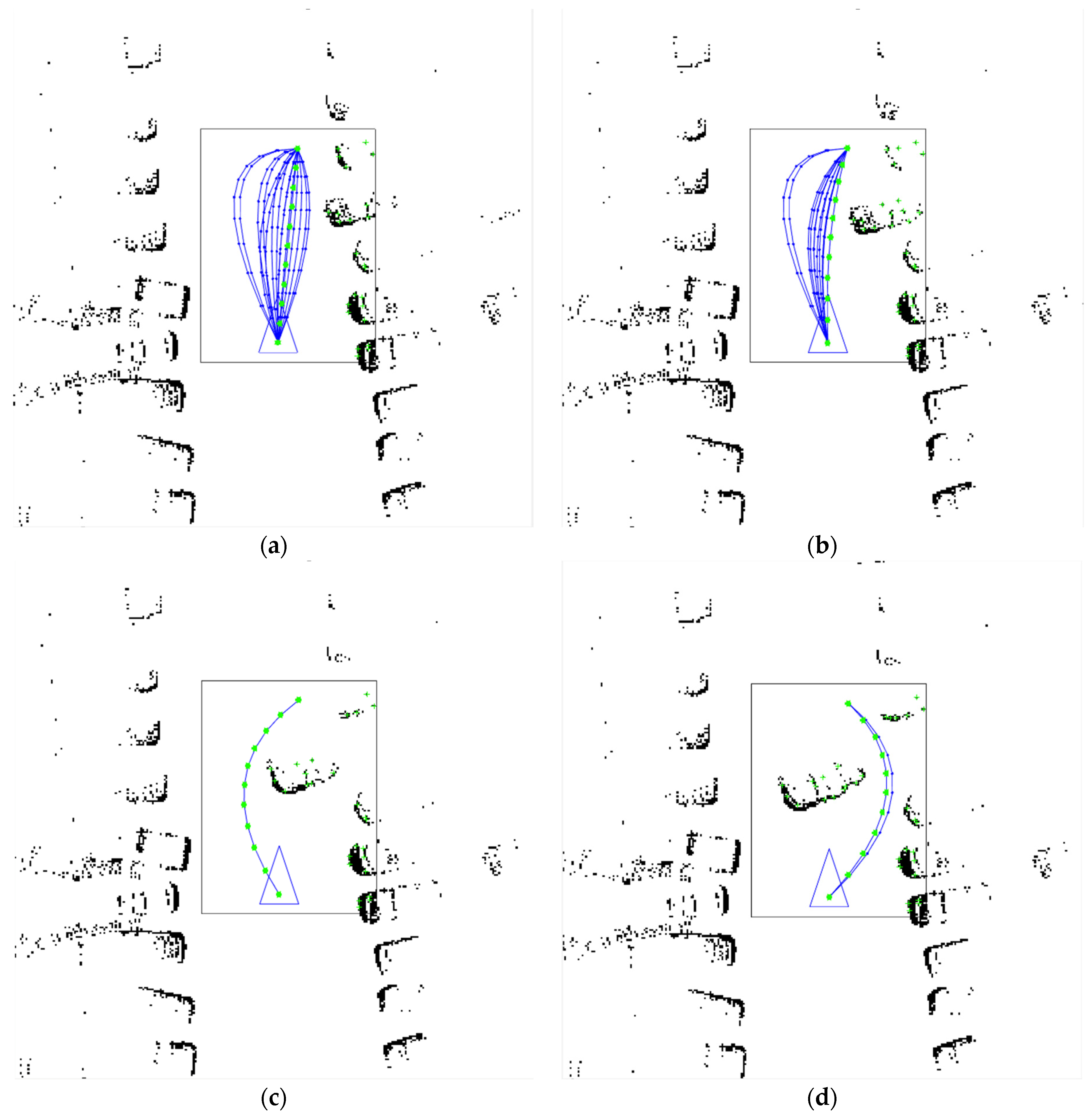
To show how the trajectory generator algorithm works, four scenarios have been selected where a car drives back and interrupts the initial trajectory (scenario 1, Figure 10a) between WPi to WPi+1 of the CICar. The scenarios (1 to 4, Figure 10) present an increasing complexity, where the trajectory generator must recalculate the set of trajectories depending of the new keypoints location.
Figure 10 shows how the trajectory generator is capable of resolving a normal traffic situation successfully. The trajectory generator module was configured with 30 iterations and a safety distance of 1 m, and the optimal trajectory criteria were set to the lowest distance travelled. In all the scenarios proposed in Figure 10, the trajectory generator module generated 30 trajectories, but the safety distance constraint only passed: 16 in scenario 1, 11 in scenario 2, 1 in scenario 3, and 2 in scenario 4. In each trajectory set the optimal trajectory was selected according to the lowest distance travelled.
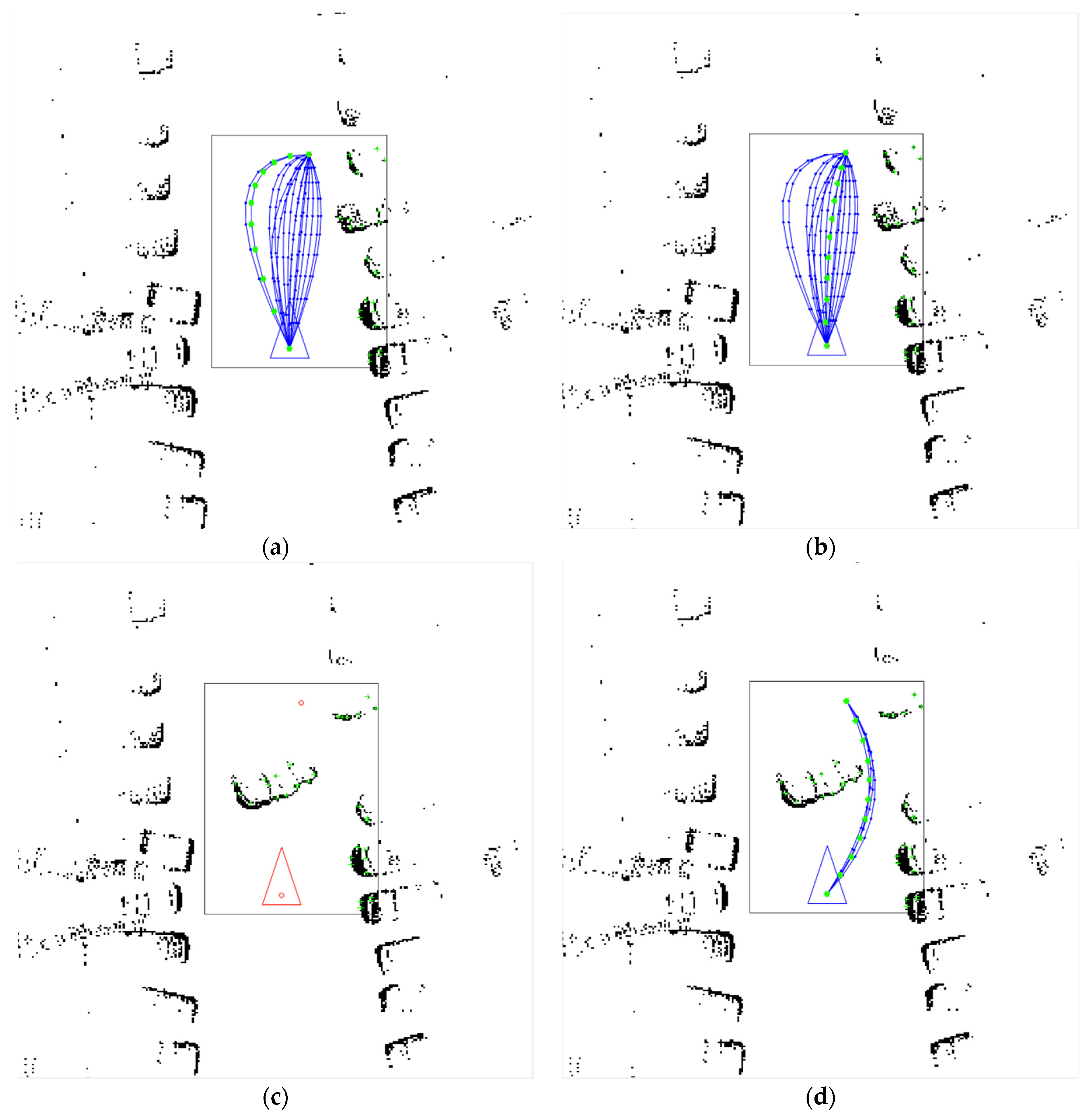
Figure 11 shows the behaviours of the trajectory generator when other criteria and parameters of the algorithm are chosen. In Figure 11a,b, the maximum angle criteria and medium trajectory criteria have been selected from scenario 1, respectively. It is possible to observe that the change in the selection criteria affect the smoothness of the trajectory. In Figure 11c,d, the number of possible trajectories was set to 25. With this change in criteria, the trajectory generator cannot avoid the obstacle and cannot supply any solution in this scenario (see Figure 8c). Nevertheless, a decrement of the safety distance to 0.5 m allows four reliable trajectories to be generated (see Figure 11d).
4. Conclusions
The Intelligent Vehicle (IV) will play a central role in the so-called Intelligent Transport Systems. For this reason, a great research effort is devoted to developing algorithms and control strategies for autonomous driving. It is essential, therefore, to have real driving platforms ready to implement and test these algorithms and control strategies.
This paper describes the work done to develop and implement low- and high-level open architectures for an autonomous vehicle: the CICar. The low-level architecture is presented in detail, and comprises a detailed description of all hardware components, sensors, and communication infrastructures on board. Also, the high-level architecture is described, which brings together those systems that provide the vehicle with a certain degree of intelligence.
Unlike other platforms presented, which use proprietary control systems, in the Intelligent Vehicles Lab we propose an approach based on well-known hardware–software development platforms for control purposes: RIO architecture and LabVIEW. This means that the current software development approach for self-driving can be easily transferred to control actions on any vehicle equipped with the general purpose control hardware proposed for the CICar.
The sensing infrastructure includes ToF cameras for lateral surveillance. This sensing technology offers advantages compared with the current 2D LIDAR, since a better characterization of the scene is possible, thus offering better capabilities such as: 3D object detection with a high frame rate, lower influence of the light conditions and shadows, and acceptable cost.
As a proof of concept, this paper shows a case study where the implementation of a PPS (path-planning system) on the CICar platform is presented. The implemented PPS uses a map to establish a global route and a local planner to solve the usual traffic issues. The global planer has been resolved by means of the development of a new heuristic algorithm based on a search for cross points (SCP) using binary maps. The SCP algorithm has improved the flexibility, the computing time, and the performance in global route computation. Furthermore, a local planner has also been presented in this work, which implements a trajectory generator based on Bezier curves, which supplies high flexibility during the resolution of unforeseen situations. The trajectory generator allows the setting of: (a) the number of possible trajectories to generate; (b) a safety distance; (c) a criterion to select the optimal trajectory. The CICar autonomous vehicle offers a comprehensible and reliable platform for autonomous driving technology development and testing, which greatly facilitates the development of technology for autonomous driving.
Concerning the PPS, we currently continue to work towards increasing the intelligence to implement it on board the vehicle. We focus our developments on: (a) the improvement of the evaluation criteria for the optimal trajectory; (b) the dynamic modification of the ROI, depending on external driving factors; (c) the incorporation of machine learning technology for the classification of the objects detected by the perception systems.
Acknowledgments
This work was partially supported by ViSelTR (ref. TIN2012-39279), DGT (ref. SPIP2017-02286) and UPCA13-2E-1929 Spanish Government projects, and the “Research Programme for Groups of Scientific Excellence in the Region of Murcia” of the Seneca Foundation (Agency for Science and Technology in the Region of Murcia-19895/GERM/15). We would like to thank Leanne Rebecca Miller for the edition of the manuscript.
Author Contributions
R.B. carried out the design and the mechanical modification of the systems on the vehicle; P.J.N conceived and designed the algorithms involved in the Path-Planning Systems. C.F. and P.A. contributed to improve the mechanical systems and operating system of the vehicle, respectively. R.B, P.J.N, C.P, and P.A. wrote and corrected the draft and approved the final version of the paper.
Conflicts of Interest
The authors declare no conflict of interest.
References
- Kala, R. On-Road Intelligent Vehicles: Motion Planning for Intelligent Transportation Systems; Elsevier Science: Amsterdam, The Netherlands, 2016. [Google Scholar]
- Flemming, B.; Gill, V.; Godsmark, P.; Kirk, B. Automated Vehicles: The Coming of the Next Disruptive Technology. In The Conference Board of Canada; Conference Board of Canada: Ottawa, ON, Canada, 2015. [Google Scholar]
- Corben, B.; Logan, D.; Fanciulli, L.; Farley, R.; Cameron, I. Strengthening road safety strategy development “Towards Zero” 2008–2020 – Western Australia’s experience scientific research on road safety management SWOV workshop 16 and 17 November 2009. Saf. Sci. 2010, 48, 1085–1097. [Google Scholar] [CrossRef]
- Engelbrecht, J.; Booysen, M.J.; Bruwer, F.J.; van Rooyen, G.-J. Survey of smartphone-based sensing in vehicles for intelligent transportation system applications. IET Intell. Transp. Syst. 2015, 9, 924–935. [Google Scholar] [CrossRef]
- Thrun, S. Toward robotic cars. Commun. ACM 2010, 53, 99. [Google Scholar] [CrossRef]
- Ibañez-Guzmán, J.; Laugier, C.; Yoder, J.-D.; Thrun, S. Autonomous Driving: Context and State-of-the-Art. In Handbook of Intelligent Vehicles; Springer: London, UK, 2012; pp. 1271–1310. [Google Scholar]
- Urmson, C.; Anhalt, J.; Bagnell, D.; Baker, C.; Bittner, R.; Clark, M.N.; Dolan, J.; Duggins, D.; Galatali, T.; Geyer, C.; et al. Autonomous Driving in Urban Environments: Boss and the Urban Challenge. J. F. Robot. 2009, 25, 1–59. [Google Scholar]
- NHTSA Federal Automated Vehicles Policy—September 2016 | US Department of Transportation. Available online: https://www.transportation.gov/AV/federal-automated-vehicles-policy-september-2016 (accessed on 29 November 2017).
- SAE J3016: Taxonomy and Definitions for Terms Related to On-Road Motor Vehicle Automated Driving Systems - SAE International. Available online: http://standards.sae.org/j3016_201401/ (accessed on 29 November 2017).
- Wei, J.; Snider, J.M.; Kim, J.; Dolan, J.M.; Rajkumar, R.; Litkouhi, B. Towards a viable autonomous driving research platform. In IEEE Intelligent Vehicles Symposium, Proceedings; Gold Coast, QLD, Australia, 2013; pp. 763–770. [Google Scholar]
- Milanés, V.; Llorca, D.F.; Vinagre, B.M.; González, C.; Sotelo, M.A. Clavileño: Evolution of an autonomous car. In Proceedings of the IEEE Conference on Intelligent Transportation Systems, Proceedings, ITSC, Funchal, Portugal, 19–22 September 2010; pp. 1129–1134. [Google Scholar]
- Grisleri, P.; Fedriga, I. The BRAiVE Autonomous Ground Vehicle Platform. IFAC Proc. Vol. 2010, 43, 497–502. [Google Scholar] [CrossRef]
- Levinson, J.; Askeland, J.; Becker, J.; Dolson, J.; Held, D.; Kammel, S.; Kolter, J.Z.; Langer, D.; Pink, O.; Pratt, V.; et al. Towards fully autonomous driving: Systems and algorithms. In IEEE Intelligent Vehicles Symposium, Proceedings; Baden-Baden, Germany, 2011; pp. 163–168. [Google Scholar]
- Liu, S.; Tang, J.; Wang, C.; Wang, Q.; Gaudiot, J.L. A Unified Cloud Platform for Autonomous Driving. Computer 2017, 50, 42–49. [Google Scholar] [CrossRef]
- Liu, S.; Tang, J.; Wang, C.; Wang, Q.; Gaudiot, J.-L. Implementing a Cloud Platform for Autonomous Driving. arXiv 2017, arXiv:1704.02696. [Google Scholar]
- NI white papers The LabVIEW RIO Architecture: A Foundation for Innovation. Available online http://www.ni.com/white-paper/10894/en/ (accessed on 14 February 2018).
- Hu, J.; Xiong, C. Study on the embedded CAN bus control system in the vehicle. In Proceedings of the 2012 International Conference on Computer Science and Electronics Engineering, ICCSEE 2012, Hangzhou, China, 23–25 March 2012; IEEE; Volume 2, pp. 440–442. [Google Scholar]
- Petrovskaya, A.; Thrun, S. Model based vehicle detection and tracking for autonomous urban driving. Auton. Robots 2009, 26, 123–139. [Google Scholar] [CrossRef]
- Navarro, P.; Fernández, C.; Borraz, R.; Alonso, D. A Machine Learning Approach to Pedestrian Detection for Autonomous Vehicles Using High-Definition 3D Range Data. Sensors 2016, 17, 18. [Google Scholar] [CrossRef] [PubMed]
- Samek, M. Practical UML Statecharts in C/C++: Event-Driven Programming for Embedded Systems; Newnes/Elsevier: Burlington, MA, USA, 2009. [Google Scholar]
- Li, L. Time-of-Flight Camera–An Introduction; Technical White Paper; Texas Instruments: Dallas, TX, USA, 2014; p. 10. [Google Scholar]
- Lange, R.; Seitz, P. Solid-state time-of-flight range camera. IEEE J. Quantum Electron. 2001, 37, 390–397. [Google Scholar] [CrossRef]
- Piñana-Díaz, C.; Toledo-Moreo, R.; Toledo-Moreo, F.; Skarmeta, A. A Two-Layers Based Approach of an Enhanced-Mapfor Urban Positioning Support. Sensors 2012, 12, 14508–14524. [Google Scholar] [CrossRef] [PubMed]
- Piñana-Diaz, C.; Toledo-Moreo, R.; Bétaille, D.; Gómez-Skarmeta, A.F. GPS multipath detection and exclusion with elevation-enhanced maps. In Proceedings of the IEEE Conference on Intelligent Transportation Systems, Proceedings, ITSC, Washintong, DC, USA, 5–7 October 2011; pp. 19–24. [Google Scholar]
- Czubenko, M.; Kowalczuk, Z.; Ordys, A. Autonomous Driver Based on an Intelligent System of Decision-Making. Cognit. Comput. 2015, 7, 569–581. [Google Scholar] [CrossRef] [PubMed]
- Chen, B.; Cheng, H.H. A Review of the Applications of Agent Technology in Traffic and Transportation Systems. IEEE Trans. Intell. Transp. Syst. 2010, 11, 485–497. [Google Scholar]
- Abdullah, R.; Hussain, A.; Warwick, K.; Zayed, A. Autonomous intelligent cruise control using a novel multiple-controller framework incorporating fuzzy-logic-based switching and tuning. Neurocomputing 2008, 71, 2727–2741. [Google Scholar] [CrossRef]
- Belker, T.; Beetz, M.; Cremers, A.B. Learning action models for the improved execution of navigation plans. Rob. Auton. Syst. 2002, 38, 137–148. [Google Scholar] [CrossRef]
- Chakraborty, D.; Vaz, W.; Nandi, A.K. Optimal driving during electric vehicle acceleration using evolutionary algorithms. Appl. Soft Comput. 2015, 34, 217–235. [Google Scholar] [CrossRef]
- Michalos, G.; Fysikopoulos, A.; Makris, S.; Mourtzis, D.; Chryssolouris, G. Multi criteria assembly line design and configuration – An automotive case study. CIRP J. Manuf. Sci. Technol. 2015, 9, 69–87. [Google Scholar] [CrossRef]
- Cunningham, A.G.; Galceran, E.; Eustice, R.M.; Olson, E. MPDM: Multipolicy decision-making in dynamic, uncertain environments for autonomous driving. In Proceedings of the IEEE International Conference on Robotics and Automation, Seatle, WA, USA, 26-30 May 2015; IEEE; Volume 2015-June, pp. 1670–1677. [Google Scholar]
- Chu, K.; Lee, M.; Sunwoo, M. Local path planning for off-road autonomous driving with avoidance of static obstacles. IEEE Trans. Intell. Transp. Syst. 2012, 13, 1599–1616. [Google Scholar] [CrossRef]
- Biswas, S.; Lovell, B.C. B-Splines and Its Applications. In Bézier and Splines in Image Processing and Machine Vision; Springer: London, UK; pp. 3–31.
- Hart, P.; Nilsson, N.; Raphael, B. A Formal Basis for the Heuristic Determination of Minimum Cost Paths. IEEE Trans. Syst. Sci. Cybern. 1968, 4, 100–107. [Google Scholar] [CrossRef]
- Dijkstra, E.W. A Note on Two Problems in Connexion with Graphs. In Numerische Mathematik; Stichting Mathematisch Centrum: Amsterdam, The Netherlands, 1959; Volume 271, pp. 269–271. [Google Scholar]
- Harris, C.; Stephens, M. A combined corner and edge detector. In Proceedings of the Fourth Alvey Vision Conference, Manchester, UK, 31 August–2 September 1988. [Google Scholar]
Figure 1.
Automation of driving elements. (a) Renault Twizy; (b) steering modification; (c) braking system modification; (d) throttle modification.
Figure 1.
Automation of driving elements. (a) Renault Twizy; (b) steering modification; (c) braking system modification; (d) throttle modification.

Figure 2.
(a) Low-level architecture; (b) rack to host the control and decision making systems.

Figure 3.
Distribution of the high-level architecture components of the CICar.

Figure 4.
(a) CICar 3D model with reference frames; (b,c) plant and side views of the perception system ranges and components.
Figure 4.
(a) CICar 3D model with reference frames; (b,c) plant and side views of the perception system ranges and components.

Figure 5.
Example of the Search for Cross Points (SCP) working between p0 and pg with initial angle θ0 = 60°. (a) Scenario without change of direction; (b) Obtained trajectory in scenario without change of direction; (c) Scenario with change of direction; (d) Obtained trajectory in scenario with change of direction.

Figure 6.
SCP applied on a real map. (a) Selection of the initial point on the real map; (b) cross points found on a binary map; (c) possible trajectories on a binary map; (d) optimum trajectory on the real map.
Figure 6.
SCP applied on a real map. (a) Selection of the initial point on the real map; (b) cross points found on a binary map; (c) possible trajectories on a binary map; (d) optimum trajectory on the real map.


Figure 7.
Local planner flowchart.

Figure 8.
(a) Local map; (b) local filtered map.

Figure 9.
Waypoints (WPi, WPi+1), ROI, and keypoints in two scenarios (a,b).

Figure 10.
(a) Scenario 1; (b) scenario 2; (c) scenario 3; (d) scenario 4 (nCurves = 30, safety distance = 1 m, criteria = minimum distance).
Figure 10.
(a) Scenario 1; (b) scenario 2; (c) scenario 3; (d) scenario 4 (nCurves = 30, safety distance = 1 m, criteria = minimum distance).

Figure 11.
(a) Scenario 1 (nCurves = 30, safety distance = 1 m, criteria = maximum angle); (b) scenario 1 (nCurves = 30, safety distance = 1 m, criteria = medium trajectory); (c) scenario 4 (nCurves = 25, safety distance = 1 m, criteria = minimum distance); (d) scenario 4 (nCurves = 25, safety distance = 0.5 m, criteria = minimum distance).


Table 1.
Capacities of an IV.
| Capacity | Means to Achieve That Capacity |
|---|---|
| Acquisition of information about the environment (at different distances) | Onboard sensors (self-positioning, obstacle detection, driver monitoring) |
| Network connection for long-distance information | |
| Vehicular interconnection | |
| Processing of environment information | Onboard software for critical analysis |
| Cloud processing for route planning, traffic control, etc. | |
| Making driving decisions | Cognitive systems |
| Agent systems | |
| Evolutionary algorithms |
Table 2.
Three categories of advanced driving automation.
| Category | Main Features | Fault Correction Rely on | Automated Driving Modes Covered |
|---|---|---|---|
| Level 3. Conditional Automation | All dynamic driving tasks are automated. The human driver is expected to act correctly when required. | Human driver | Some driving modes: |
| Parking maneuvers | |||
| Low speed traffic jam | |||
| Level 4. High Automation | All dynamic driving tasks are automated. The human driver is not expected to act correctly when required. | System | Some driving modes: |
| High-speed cruising | |||
| Level 5. Full Automation | All dynamic driving tasks are automated for any type of road and environmental conditions usually managed by a human driver. | System | All driving modes |
| Urban driving |
Table 3.
Some platforms for autonomous driving development.
| PLATFORM | Vehicle Basis | Automated Systems | Control System | Sensors | Performances | Navigation |
|---|---|---|---|---|---|---|
| BOSS (DARPA) | Chevrolet Thaoe | Steering Brake Throttle | Proprietary (based on multiprocessor system) | 1 HD 3D LIDAR 4 Cameras 6 radars 8 2D LIDAR 1 Inertial GPS navigation system. | Obstacle avoidance Lane keeping Crossing detection | Anytime D* Algorithm |
| JUNIOR (DARPA) | VW Passat wagon | Steering Brake Throttle | Proprietary (based on multiprocessor system) | 1 HD 3D LIDAR 4 Cameras 6 radars 2 2D LIDAR 1 Inertial GPS navigation system. | Object detection Pedestrian detection | Moving Frame |
| BRAiVE (VisLab) | VW Passat | Steering Brake Throttle | Proprietary dSpace | 10 cameras 4 lasers 16 laser beams 1 radar 1 Inertial GPS navigation system. | Close loop manoeuvring | NA |
| AUTOPIA | CITRÖEN C3 Pluriel | Steering Brake Throttle | Proprietary ORBEX (based on fuzzy coprocessor) | 2 front cameras 1 RTK-DGPS+IMU | Following a leading vehicle Pedestrian detection | Fuzzy logic |
Table 4.
Sensors features of the perception system.
| Sensor | Characteristics and Configurations |
|---|---|
| SICK LASER scanner 2D TIM551 | Operating range: 0.05 m ... 4 m, Aperture angle: 270° |
| LIDAR VELODYNE HDL64 scanner 3D | 120 m range, 1.3 Million Points per Second, 26.9° Vertical FOV |
| Prosilica GT1290 cam | 1.2 Megapixel Ethernet gigabit, RJ45 Ethernet connector, colour |
| DGPS | GPS aided AHRS |
| ToF Sentis3D-M420Kit cam | Range Indoor: 7 m Outdoor: 4 m, Horizontal FOV: 90° |
| IMU Moog Crossbow NAV440CA-202 | Pitch and roll accuracy of < 0.4°, Position Accuracy < 0.3 m |
| EMLID RTK GNSS Receiver | 7 mm positioning precision |
Table 5.
Calculation of angles θ1, θ2, depending on the direction.
| Directions | Angle θ1 | Angle θ2 |
|---|---|---|
| N | −180 + θ0 | −θ0 |
| S | θ0 | 180 − θ0 |
| E | θ0 | −θ0 |
| W | −180 + θ0 | 180 − θ0 |
© 2018 by the authors. Licensee MDPI, Basel, Switzerland. This article is an open access article distributed under the terms and conditions of the Creative Commons Attribution (CC BY) license (http://creativecommons.org/licenses/by/4.0/).
Share and Cite
MDPI and ACS Style
Borraz, R.; Navarro, P.J.; Fernández, C.; Alcover, P.M. Cloud Incubator Car: A Reliable Platform for Autonomous Driving. Appl. Sci. 2018, 8, 303. https://doi.org/10.3390/app8020303
AMA Style
Borraz R, Navarro PJ, Fernández C, Alcover PM. Cloud Incubator Car: A Reliable Platform for Autonomous Driving. Applied Sciences. 2018; 8(2):303. https://doi.org/10.3390/app8020303
Chicago/Turabian StyleBorraz, Raúl, Pedro J. Navarro, Carlos Fernández, and Pedro María Alcover. 2018. "Cloud Incubator Car: A Reliable Platform for Autonomous Driving" Applied Sciences 8, no. 2: 303. https://doi.org/10.3390/app8020303
Note that from the first issue of 2016, this journal uses article numbers instead of page numbers. See further details here.