Potential of TCPInSAR in Monitoring Linear Infrastructure with a Small Dataset of SAR Images: Application of the Donghai Bridge, China


1
Department of Land Surveying and Geo-Informatics, The Hong Kong Polytechnic University, Hong Kong 999077, China
2
College of Resources and Environmental Science, Hunan Normal University, No. 36 Lushan Road, Changsha 410081, China
3
Key Laboratory of Geospatial Big Data Mining and Application, Hunan Province, Changsha 410081, China
4
School of Geosciences and Info-Physics, Central South University, Changsha 410083, China
*
Author to whom correspondence should be addressed.
Appl. Sci. 2018, 8(3), 425; https://doi.org/10.3390/app8030425
Submission received: 14 February 2018
/
Revised: 6 March 2018
/
Accepted: 6 March 2018
/
Published: 19 March 2018
Abstract
:Reliably monitoring deformation associated with linear infrastructures, such as long-span bridges, is vitally important to assess their structural health. In this paper, we attempt to employ satellite interferometric synthetic aperture radar (InSAR) to map the deformation of Donghai Bridge over a half of an annual cycle. The bridge, as the fourth longest cross-sea bridge in the world, located in the north of Hangzhou Bay, East China Sea where the featureless sea surface largely occupied the radar image raises challenges to accurately co-register the coherent points along the bridge. To tackle the issues due to co-registration and the limited number of synthetic aperture radar (SAR) images, we adopt the termed temporarily-coherent point (TCP) InSAR (TCPInSAR) technique to process the radar images. TCPs that are not necessarily coherent during the whole observation period can be identified within every two SAR acquisitions during the co-registration procedure based on the statistics of azimuth and range offsets. In the process, co-registration is performed only using the offsets of these TCPs, leading to improved interferometric phases and the local Delaunay triangulation is used to construct point pairs to reduce the atmospheric artifacts along the bridge. With the TCPInSAR method the deformation rate along the bridge is estimated with no need of phase unwrapping. The achieved result reveals that the Donghai Bridge suffered a line-of-sight (LOS) deformation rate up to −2.3 cm/year from January 2009 to July 2009 at the cable-stayed part, which is likely due to the thermal expansion of cables.
1. Introduction
As is well known, the study of ground deformation experienced a major breakthrough in 1990s with the development of space-based observation techniques. An important element in this has been the advent of synthetic aperture radar interferometry (InSAR) that can reveal details of the deformation in complex areas [1,2,3,4,5,6]. In order to overcome the limitations of the conventional InSAR technique, i.e., spatial-temporal decorrelation and atmospheric artifacts, the persistent scatterer InSAR (PSInSAR) technique was developed in late 1990s [7,8]. The technique takes the phase difference between adjacent pixels that have strong backscatterering features during the whole time span as observations in order to suppress the spatial-temporal decorrelation and atmospheric artifacts. Many algorithms have subsequently been proposed to enhance the robustness and applicability of PSInSAR [9,10,11]. Over the years the application of PSInSAR has been widely performed, ranging from monitoring ground deformation in urban and nonurban areas (e.g., [12,13,14,15,16,17,18]) to monitoring single infrastructures, such as dams and buildings (e.g., [19,20,21,22]). However, the PSInSAR technique generally needs more than 30 scenes of SAR images to guarantee the validity of the selected coherent points [8]. Additionally, the accuracy of PSInSAR-derived displacement benefits from a reliable searching in the predefined solution space, which depends on the high density of coherent points. This is, however, not always satisfied in the investigation of linear infrastructures, such as bridges, motorways, and pipelines, especially with moderate-resolution SAR data [23,24,25,26,27,28,29].
Temporal coherent point InSAR (TCPInSAR) is a well-developed multi-temporal technique that can identify and co-register the coherent points with a small number of SAR acquisitions and estimate the surface displacement without the requirement of either 3D phase unwrapping or solution space searching [30,31]. The approach has been successfully applied in the monitoring of urban ground deformation, mining-induced subsidence, interseismic deformation, and landslides, with a large or moderate set of observations [32,33,34,35]. In this paper, we experiment to extend the application of the TCPInSAR technique to monitor the deformation of linear infrastructure with emphasis on using a small dataset of SAR images. The studied linear infrastructure is the Donghai Bridge, which is located in the north of Hangzhou Bay in the East China Sea and has a length of 32.5 km over the sea and 3.7 km over the land, respectively (Figure 1). The width of the bridge is 31.5 m, including twin decks and a six-lane dual carriageway. Donghai Bridge was built by using the concrete placing method, with construction starting on 26 June 2002, with completion after 35 months. There is a two-way main navigation hole in the bridge, which has the navigable clear height of 40 m and allows the navigation of 5000 t ships. This section of the bridge is suspended by 192 cables, which are supported by two towers with heights of 159 m. As the fourth longest cross-sea bridge in the world, the Donghai Bridge links mainland Shanghai with Yangshan Deep-Water Port.
Reliably monitoring the deformation of such a long-span bridge is of great importance to assess its structural safety [24]. Compared with continuous GPS data, which have been widely used to monitor long bridges, InSAR measurements can provide much denser spatial samples along the bridge with no need of installing ground instruments. However, as a crucial step in InSAR processing, accurate co-registration between SAR images is challenging over areas largely occupied by the featureless sea surface. In the conventional method, where evenly-distributed windows are used to obtain the offsets between the master and slave images, the offsets over the sea area can distort the co-registration polynomial fitting, even though there is a predefined threshold to remove the inaccurately-estimated offsets. Such errors can be avoided in TCPInSAR processing since the TCPs are co-registered only according to their own offsets. To tackle the atmospheric artifacts along the long-span bridge surrounded by sea water, we limit the maximum length of arcs (or point pairs) by utilizing local Delaunay triangulation to construct arcs. Equipped with these processing strategies, TCPInSAR has the potential to monitor the deformation of long-span cross-sea bridges caused by foundation settlement, bridge deck creep, stress relaxation, as well as environmental conditions, such as temperature, wind, tide, and others.
2. Methodology
2.1. Data Selection
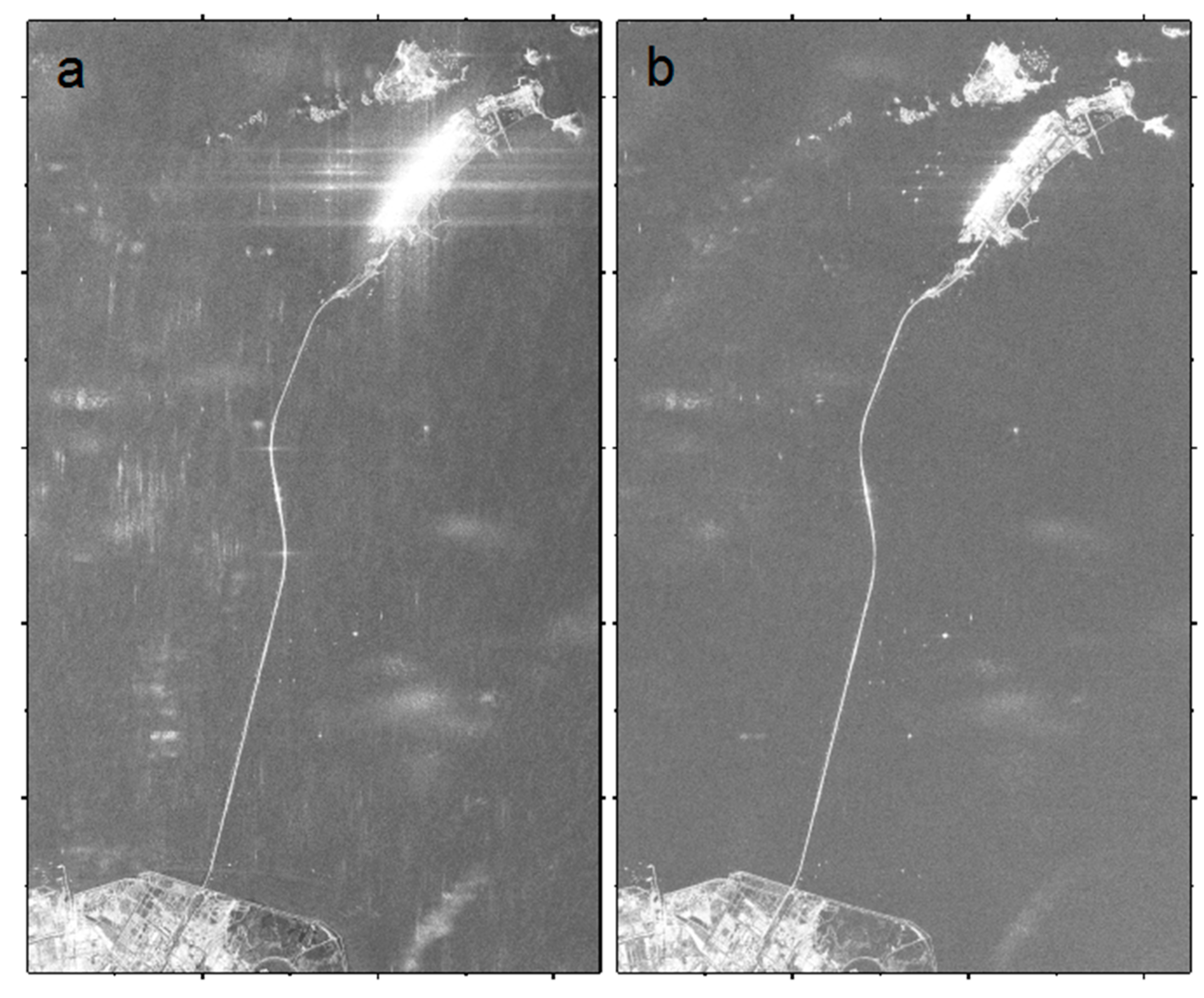
Over the Donghai Bridge we have collected a set of data acquired by a Phased Array type L-band Synthetic Aperture Radar (PALSAR) on the Advanced Land Observing Satellite (ALOS) under fine beam double (FBD) polarization. Compared to the C-band data, e.g., the Environmental Satellite/Advanced Synthetic Aperture Radar (ENVISAT/ASAR) data and RADARSAT-1/2 data, the L-band PALSAR data can better resist the decorrelation (Figure 2). When we look into the PALSAR data we further find that the Horizontal Vertical (HV)-polarized data (Figure 2b) has better performance on minimizing the amplitude ambiguity in the sea area and suppressing the side lobe effects on the island than the Horizontal Horizontal (HH)-polarized data (Figure 2a). Hence, we finally chose four HV PALSAR datasets as observations to determine the deformation rate of the Donghai Bridge. From the six interferograms generated by the four images we selected three single-master pairs with relatively short perpendicular baselines (see Table 1).
2.2. Temporarily-Coherent Point Identification
Temporarily coherent points (TCPs) are the points in the interferograms that can remain coherent during one or several intervals of SAR acquisitions, but do not need to be visible over the whole time span. We identify these points primarily based on the fact that the offset estimation at the points with high coherence is less affected by window size and oversampling factors compared with low coherent points. By statistical analysis of offset vectors estimated with changing window sizes at each pixel, the TCPs can be isolated. The theoretical analysis and real data test of the method can be found in [30,36]. Here, only the key steps of the method are listed briefly. First, the scene is divided into a set of large patches and the range and azimuth offsets for each patch are estimated to determine the offset polynomial functions between two images. Second, the estimated offset is taken as an initial input and cross-correlation is implemented at every single pixel using smaller patches. We can obtain an offset matrix:
where is the offset of pixel (). TCP candidates can be selected according to a 2D histogram:
where is the tolerated interval used in the 2D histogram. Third, the TCP candidates are further evaluated by changing the size of the patches and the oversampling factor for the cross-correlation estimation to find sub-pixel offsets. For the sake of simplicity, a fixed oversampling factor can be used. We can obtain a set of offsets for a given TCP candidate (). The TCP candidates whose standard errors of offsets are less than 0.1 pixels, which is usually taken as a required co-registration accuracy, are selected:
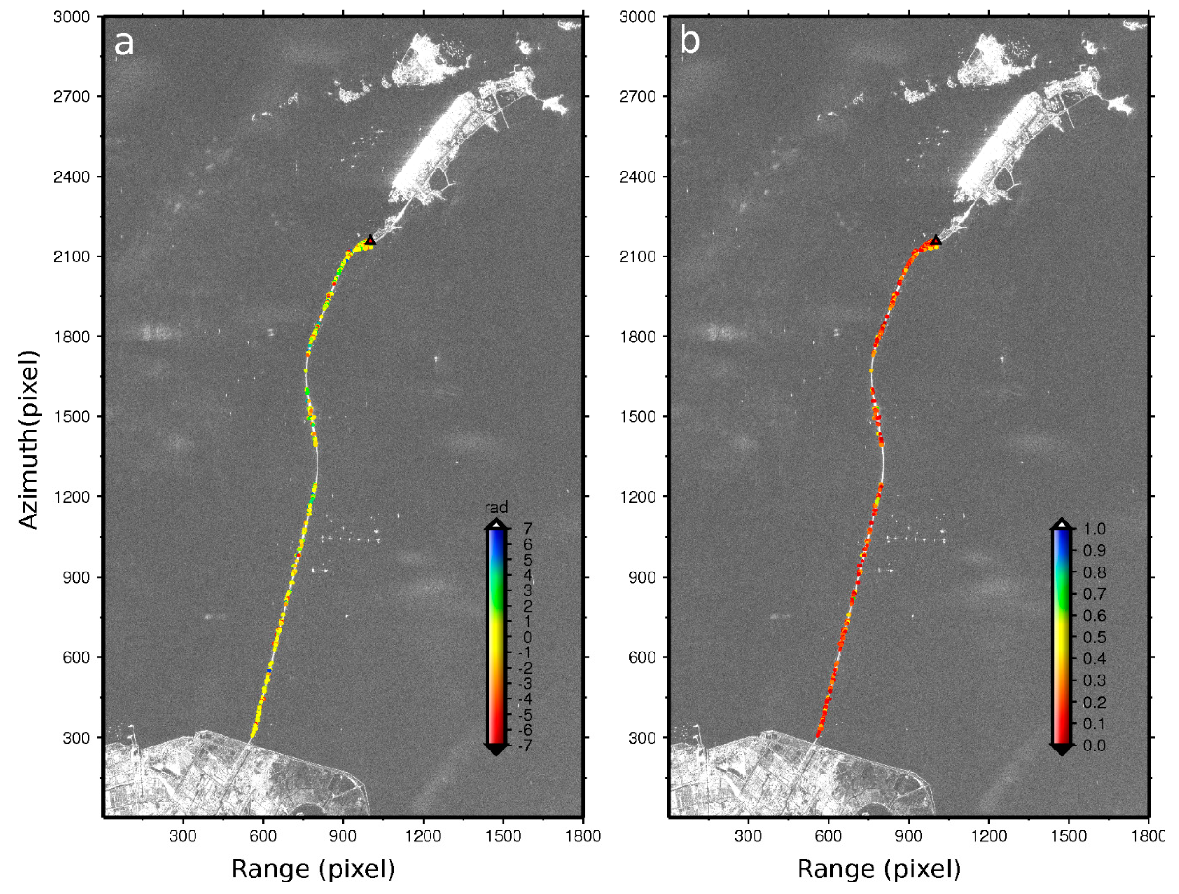
Figure 3a shows an example of the 2D histogram of the offsets estimated for an image pair where the color shows the number of points with the corresponding azimuth and range offsets. The histograms of the standard errors of the range and azimuth offsets by using different window sizes (from 256 to 32 with a step of 16) are exhibited in Figure 3b,c, respectively. Fourth, a smooth polynomial is used to fit the offsets of TCP candidates, and the TCPs are finally identified by discarding pixels whose offsets do not fit the polynomial well. An interpolator kernel is employed to resample the TCPs in the slave image based on the polynomial estimated especially from the TCPs. The TCPs identified from two interferograms are usually under different range/Doppler image coordinates. To perform time series analysis, these points should be under the same reference frame. By coincidence in this study the selected interferograms are with the same master image, therefore, no more work needs to be performed to combine the selected TCPs. The TCPs that remain coherent in all image pairs are shown as the dots in Figure 4a,b. With the proposed strategies, the coherence at the TCPs has an improvement of 0.12 on average.
2.3. Temporarily Coherent Point Co-registration
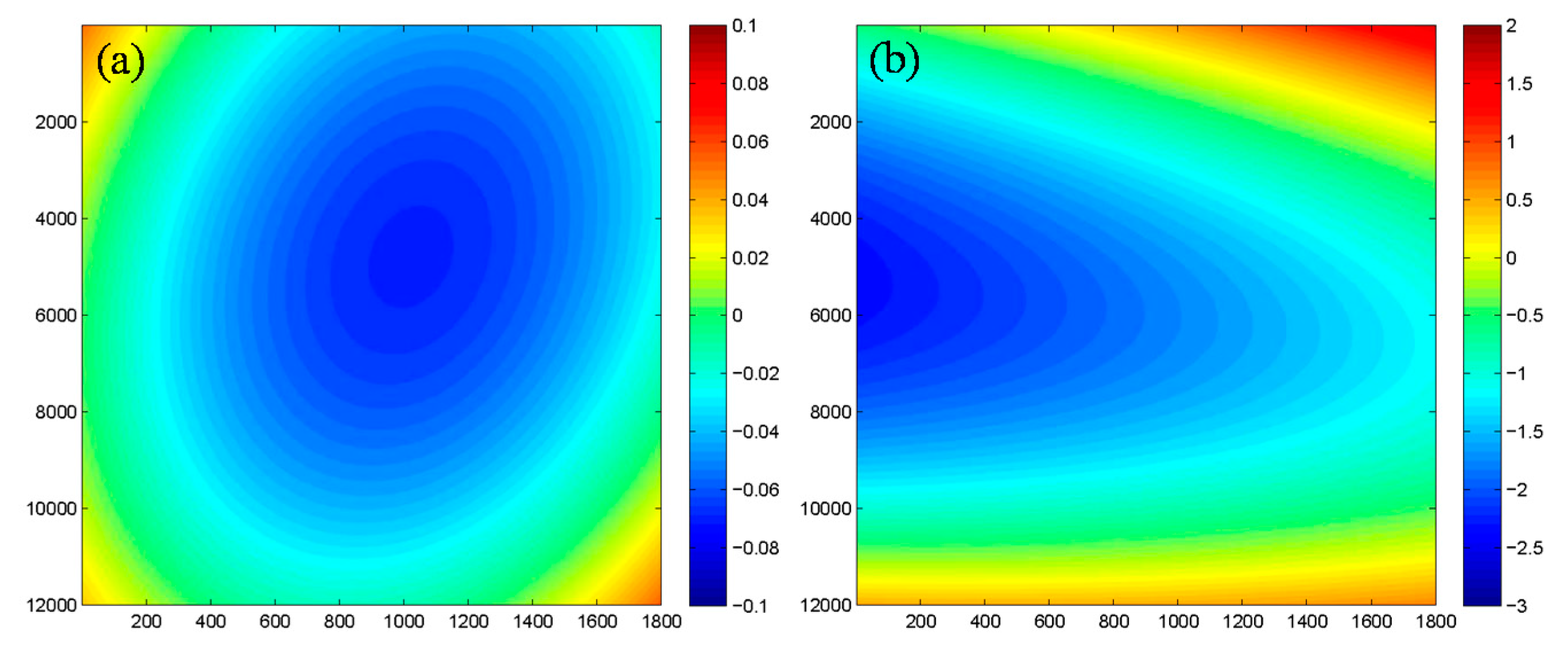
Co-registration of SAR images is the first and vital step in the InSAR processing chain. However, the fact that long cross-sea bridges are usually surrounded by sea area poses a challenge to the conventional co-registration method which employs distributed windows over the whole image to estimate the offsets between corresponding pixels [36,37]. Since the large portion of pixels is located in the sea, the offsets estimated from these pixels are not stable and vary randomly according to the changing window sizes although their signal-to-noise ratios (SNRs) appear to be higher than the threshold. In order to overcome the distortions on the coherent points caused by conventional co-registration methods, we determine the offset polynomial that will be used for resampling slave images only from the offsets at the identified TCPs [38]. A comparison is made between the offsets estimated from the identified TCPs and evenly-distributed windows over the whole image, where the window size is 256 and the oversampling factor is 2. The result indicates that the global co-registration polynomial can introduce positioning bias to the TCPs, with an extreme value of about 3 pixels in the azimuth direction (see Table 2 and Figure 5).
2.4. Temporarily-Coherent Point Network
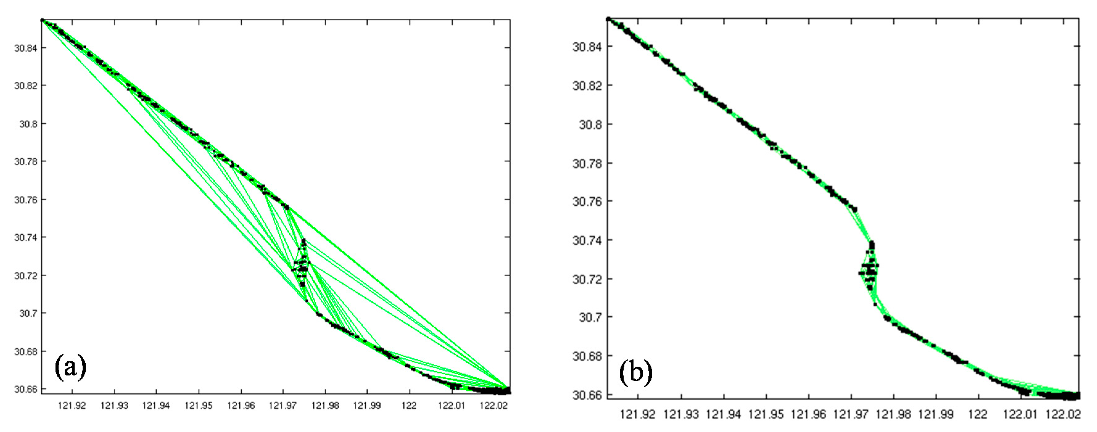
Once the TCPs are identified and co-registered, a network that indicates upon which pairs of TCPs the estimation will be performed needs to be constructed. Delaunay triangulation has been widely used for this purpose. However, Delaunay triangulation defines a triangle network under the condition that all the circumcircles of all the triangles in the net are empty without considering the maximum length of the arcs (see Figure 6a). Although arcs which are longer than a certain length will be removed in the final step, points are not connected with an optimized arc length. If only points in a small region are considered to be connected, arcs with proper lengths can be constructed without increasing the very large complexity, and the density of arcs can also be improved. Figure 6b shows the connection using local Delaunay triangulation. A grid with an interval of 100 m is placed over the interferogram and points in a circle with a radius of 500 m centered at the grid node are selected and connected.
2.5. Least Squares Model with Outlier Detector
From wrapped phase differences at arcs, the parameters of interest, i.e., the deformation and topographic residuals, can be estimated, where the phase ambiguity is usually resolved by solution space searching [8], 3D phase unwrapping [10], or integer least squares [9]. However, the success rate can never be guaranteed. In TCPInSAR, instead of resolving the ambiguity, we detect and remove it as an outlier. The strategy is mainly based on the fact that when we conduct least squares directly on the observations at arcs, arcs having phase ambiguity in certain observations will have abnormally large residuals. Therefore, we can identify and delete arcs with non-zero phase integers by diagnosing the least squares residuals. Moreover, since we just need to know whether the arc has phase ambiguity or not, rather than the exact location of the ambiguity, the outlier detection procedure can be simplified and implemented very efficiently. The details of the model used in TCPInSAR can be found in [31]. Here we just recall the model briefly. Supposing that differential interferograms with temporal baselines of have been generated from a set of SAR images over the study area, for an arc formed by connecting TCP x and TCP y, observation equations can be written with interferometric pairs as follows:
where is the conversion factor for the differential elevation error (), is the conversion factor for the relative deformation rate (), and is the differential part of the phase components related to atmospheric delay and other noises. The differential deformation rates of the arc for all the temporal baselines can be treated as constant, i.e., represents the deformation rate during the whole temporal interval. The Equation (4) can be rewritten in the matrix form as follows:
where:
The unknown parameters can be solved by the LS approach, which can be expressed by:
where denotes the estimated quantities, and is the prior weight matrix, which can be obtained by taking the inverse of the variance matrix of the double-difference phases. The estimated quantities for can be derived by:
The residuals of the measurements can be derived by:
The variance matrices of the estimated quantities can be derived by:
After the LS solution for each arc, an outlier detector is applied to check if the phase measurements for the arc have phase ambiguities [39]:
where denotes the maximum value in a vector or matrix and is a constant, usually chosen as 3.
Both the LS residuals and variance components for the arc are used for such a quality check. For subsequent analysis, the unacceptable arcs are discarded. After deriving the parameters (i.e., elevation-error and deformation-rate increments) of all the valid arcs, we can determine the parameters (i.e., elevation errors and deformation rates) at all TCPs with respect to a reference point.
3. Results and Discussions
The least squares estimation of deformation rates of the identified TCPs is shown in Figure 7a. The reference point was selected at an island which was assumed to be stable (shown as the triangle in Figure 7c). It is observed that the Donghai Bridge experienced a deformation range from −2.3 to 0.5 cm/year along the line-of-sight (LOS) direction, equaling to the cumulative deformation between −1.2 and 0.3 cm during the investigated period. For most of the body of the bridge, which is built on the piers, the deformation is detected within about 1 cm/year. Figure 7b shows an example of this pier-stayed bridge. However, an obvious deformation rate appeared on a cable-stayed bridge (Figure 7e) over the main navigation channel, of up to −1.2 cm (see Figure 7d).
3.1. The Density of Temporarily-Coherent Points
From Figure 7 we find that the identified TCPs were not evenly distributed along the bridge. In some parts of the bridge no TCP was selected. We mainly attribute this to three possible reasons. (1) The strike of the bridge. The relative position between the sensor and scatterers on the bridge will affect the back-scatterering characterization, resulting in no detectable scatterers on the curved part of the bridge, which is located near the cable-stayed portion; (2) The distribution of vehicles on the bridge during the acquisition time. Since the Donghai Bridge connected with the world-famous deep-water port, most of the vehicles running on the bridge are heavy trucks carrying standardized containers. The moving trucks may decorrelate the signals in some parts of the bridge; (3) The effect of side lobes. The proposed TCP selection method is a patch-based method, and it is possible that a strong scatterer may dominate in several neighboring patches leading to a false estimation of the offset at some pixels.
3.2. The Co-Registration of Temporarily-Coherent Points
It is expected that the co-registration offset derived from the TCPs is superior to that derived from the evenly-distributed window. Figure 4a exhibits that the difference between the interferometric phases of the resampled TCP from the conventional and TCP polynomials (Table 2). It is observed that the phase difference can be up to more than . Since the conventional polynomials were estimated from the windows over the whole image, which is dominated by the water, the offsets from the pixels on the water can be very unreliable and degrade the co-registration results. By using the TCP polynomials, an improvement in coherence can be achieved for all the TCPs (see Figure 4b), with an average value of about 0.12.
It should be highlighted that the displacement signal would not be removed or reduced by the co-registration using only coherent points along the bridge. Indeed, the pixel offset tracking method has always been used to monitor the ground deformation associated with geophysical phenomena, such as earthquakes [40]. However, this method can generally reach an accuracy of 1/30 pixel, equaling to about 30 cm LOS deformations when PALSAR FBD images are used. This level of precision is insufficient to detect the bridge’s deformation of several centimeters. Therefore, the TCP co-registration would not affect the follow-on deformation estimation.
3.3. Precision of the Results
For the estimated difference deformation rate at arcs, the posterior root-mean-square (RMS) is about 0.8 mm/year. Since only three interferograms are used in this case study, the RMS may lack statistical meaning and large bias might exist between the “true” RMS and the estimated one. In a practical view that the island at the one end of the bridge should keep stable, it is possible to use the points on the island to validate the result. Assuming that no deformation occurred on the island, the RMS of deformation rate of the points on the island is 1.2 mm/year.
The errors of the InSAR-derived deformation rate can be partly induced by the single master used in the three interferograms. The atmospheric delay and other noises in the master could be propagated into the interferograms, which will behave as an accumulation rather than neutralizing the estimation of the deformation rate. In addition, it is observed in Table 1 that the perpendicular baselines of the three interferograms increase with the time intervals of the three interferograms. This, however, is not in favor of the solution of the LS approach (i.e., Equation (9)), resulting in a possible indistinguishable relation between the elevation error and the deformation rate.
3.4. Discussion
It has been mentioned that the largest deformation rate occurred on the long span cable-stayed bridge (Figure 7a). The cable-stayed bridge is known as a temperature sensitive structure [41]. The difference in the temperature of cable and beam will influence the cable force and elevation of the main beam [42]. Although there are no public results on the temperature effects on the Donghai Bridge especially the cable-stayed section, the studies on the similar bridges show that the changes of elevation caused by the variation of temperature are up to several centimeters [43]. The used PALSAR data were acquired at 10:23 pm local time in January, February, April, and July, respectively, and the mean night-time temperature in those months were 1 °C, 1 °C, 10 °C and 23 °C. The bridge load during the specific acquisition time (i.e., 10:23 p.m.) is much smaller compared to that in daytime. It can be concluded that the large deformation rate on the cable-stayed bridge are mainly caused by the thermal expansion. The width of the cable-stayed bridge is nearly 260 m, resulting in a maximum vertical deflection of 0.52 m. Therefore, the detected motion of 1.2 cm would not cause any damage to the bridge stability.
In this study we focus on the testing of the performance of TCPInSAR with a small dataset of SAR images, therefore, only four images are employed which cover nearly half a year. However, at least a 1.5-year cycle is required to establish the relationship between the deformation and temperature [44]. This will be conducted in future work by involving a large dataset of SAR images.
It should be highlighted that cross-heading data can be more beneficial to the monitoring of the Donghai Bridge than the single-track data. The InSAR LOS deformations of a bridge can be constituted by three components, including the vertical component, the longitudinal components (i.e., the deformation along the longitudinal axis of the bridge), and the transversal component (i.e., the deformation perpendicular to the longitudinal axis of the bridge). The longitudinal deformation is mainly induced by thermal expansion [44,45]. We can observe in Figure 7 that the longitudinal direction of the cable-stayed bridge is nearly north, but the longitudinal direction of the other parts of the bridge (i.e., the pier-stayed bridge) is north by east, nearly parallel to the azimuth direction of the ascending PALSAR data. Therefore, the longitudinal deformation of the pier-stayed bridge might be missed by the ascending data but can be measured by the descending data [46].
We can also observe in Figure 7b that, in the pier-stayed part of the bridge, there are also some relatively large deformation rates (~1 cm/year). Since the bridge is located in a very rough sea environment it suffers many serious effects. The seasonal winds and the tide could cause the transversal deformation of the bridge, and the foundation settlement could cause the vertical deformation of the bridge. Both components are quite suitable to be monitored by the ascending PALSAR data. Therefore, it can be inferred that the seasonal winds, the tide, and the foundation settlement all contribute to the deformation of the Donghai Bridge in addition to the thermal expansion. More environmental materials and collaboration with the bridge engineers are needed to draw a more reliable conclusion on the safety of the bridge.
4. Conclusions
This paper presented a study of the TCPInSAR technique in the investigation of the deformation of a linear infrastructure (i.e., the Donghai Bridge in China) based on only four ascending PALSAR images. Compared to the commonly-used PSInSAR technique, the TCPInSAR can identify the coherent points with a small dataset of SAR images and provide reliable deformation measurements without the error-prone phase unwrapping procedure. In addition, TCPInSAR will provide tools to achieve better co-registration between SAR images that are dominated by the low coherent ground objects, such as water. The main conclusions of this study can be summarized as follows:
- (1)
- The results of the experiment have demonstrated the capability and precision of the TCPInSAR method in monitoring linear infrastructure. An average improvement in coherence of about 0.12 has been achieved by the TCP co-registration compared to the conventional globe co-registration. Up to three pixels of the differences can be found between the azimuth offsets derived from identified TCPs and evenly-distributed windows over the whole image, indicating that an un-neglected basis would be caused by the globe co-registration in the sea area. By assuming the TCPs on the island being stable, the RMS of the TCPInSAR-derived deformation rate is 1.2 mm/year, partly due to the single master used in the four interferograms. Since we only employed four PALSAR images with moderate resolution, this is acceptable precision in the monitoring of linear infrastructure.
- (2)
- Up to −1.2 cm cumulative LOS deformation (i.e., a −2.3 cm/year LOS deformation rate) has been detected in the cable-stayed section of the Donghai Bridge during January and July 2009. It is found that the deformation is highly relevant to the local temperature. This is expected since the longitudinal deformation of a bridge will be caused by the thermal expansion of the cable-stayed part. However, due to the great similarity between the direction of the pier-stayed part of the bridge and the azimuth direction of the used ascending PALSAR data, the longitudinal deformation is underestimated in this study. On the other hand, the detected ~1 cm/year deformation of the pier-stayed bridge can be constituted by the transversal deformation associated with the seasonal winds and the tide, as well as the vertical deformation associated with the foundation settlement. Although further investigation should be carried out with more SAR images and environmental materials, this study provides significant insights on the dynamics of the Donghai Bridge.
Acknowledgments
The ALOS PALSAR data were provided by the Japan Aerospace Exploration Agency (JAXA). The research was supported by the National Natural Science Foundation of China (nos. 41774023, 41704001, 41674010), the Research Grants Council (RGC) of the Hong Kong Special Administrative Region (Project Nos. PolyU 152214/14E, PolyU 152043/14E), the Science and Technology Project of Hunan Province (no. 2016SK2002), the Project of Education Department of Hunan Province (no. 16K053), and the Land and Resources Research Project of Hunan Province (No. 2017-13). We appreciate the two anonymous reviewers for their comments and suggestions which greatly improved the manuscript.
Author Contributions
L.Z., Q.S. and J.H. conceived, designed, and performed the experiments; Z.L. and Q.S. contributed to the analysis and discussions of the results; and L.Z. drafted the manuscript. All authors reviewed and approved the manuscript.
Conflicts of Interest
The authors declare no conflict of interest.
References
- Massonnet, D.; Rossi, M.; Carmona, C.; Adragna, F.; Peltzer, G.; Feigl, K.L.; Rabaute, T. The displacement field of the Landers earthquake mapped by radar interferometry. Nature 1993, 364, 138–142. [Google Scholar] [CrossRef]
- Goldstein, R.M.; Engelhardt, H.; Kamb, B.; Frolich, R.M. Satellite radar interferometry for monitoring ice sheet motion: Application to an Antarctic ice stream. Science 1993, 262, 1525–1530. [Google Scholar] [CrossRef] [PubMed]
- Wicks, C.; Thatcher, W.; Dzurisin, D. Migration of fluids beneath Yellowstone Caldera inferred from satellite radar interferometry. Science 1998, 282, 458–462. [Google Scholar] [CrossRef] [PubMed]
- Ding, X.L.; Liu, G.X.; Li, Z.W.; Chen, Y.Q. Ground subsidence montoring in Hong Kong with satellite SAR interferometry. Photogram. Eng. Remote Sens. 2004, 70, 1151–1156. [Google Scholar] [CrossRef]
- Lu, Z.; Kwoun, O.; Rykhus, R. Interferometric synthetic aperture radar (InSAR): Its past, present and future. Photogram. Eng. Remote Sens. 2007, 73, 217–221. [Google Scholar]
- Hu, J.; Ding, X.L.; Zhang, L.; Sun, Q.; Li, Z.W.; Zhu, J.J.; Lu, Z. Estimation of 3-D surface displacement based on InSAR and deformation modeling. IEEE Trans. Geosci. Remote Sens. 2017, 55, 2007–2016. [Google Scholar] [CrossRef]
- Ferretti, A.; Prati, C.; Rocca, F. Nonlinear subsidence rate estimation using permanent scatterers in differential SAR interferometry. IEEE Trans. Geosci. Remote Sens. 2000, 38, 2202–2212. [Google Scholar] [CrossRef]
- Ferretti, A.; Prati, C.; Rocca, F. Permanent scatterers in SAR interferometry. IEEE Trans. Geosci. Remote Sens. 2001, 39, 8–20. [Google Scholar] [CrossRef]
- Kampes, B.N.; Hanssen, R.F. Ambiguity resolution for permanent scatterer interferometry. IEEE Trans. Geosci. Remote Sens. 2004, 42, 2446–2453. [Google Scholar] [CrossRef]
- Hooper, A.; Segall, P.; Zebker, H. Persistent scatterer interferometric synthetic aperture radar for crustal deformation analysis, with application to Volcan Alcedo, Galapagos. J. Geophys. Res. 2007, 112, B07407. [Google Scholar] [CrossRef]
- Ferretti, A.; Fumagalli, A.; Novali, F.; Prati, C.; Rocca, F.; Rucci, A. A new algorithm for processing interferoemtric data-stacks: SqueeSAR. IEEE Trans. Geosci. Remote Sens. 2011, 49, 3460–3470. [Google Scholar] [CrossRef]
- Hilley, G.; Burgmann, R.; Ferretti, A.; Novali, F.; Rocca, F. Dynamics of slow-moving landslides from permanent scatterer analysis. Science 2004, 304, 1952–1956. [Google Scholar] [CrossRef] [PubMed]
- Dixon, T.; Amelung, F.; Ferretti, A.; Rocca, F.; Novali, F.; Wdowinski, S. New Orleans subsidence and relation to flooding after Hurricane Katrina, as measured by space geodesy. Nature 2006, 441, 587–588. [Google Scholar] [CrossRef] [PubMed]
- Zhao, Q.; Lin, H.; Jiang, L.; Chen, F.; Cheng, S. A study of ground deformation in the Guangzhou urban area with persistent scatterer interferometry. Sensors 2009, 9, 503–518. [Google Scholar] [CrossRef] [PubMed]
- Hu, J.; Ding, X.L.; Li, Z.W.; Zhang, L.; Zhu, J.J.; Sun, Q.; Gao, G.J. Vertical and horizontal displacements of Los Angeles from InSAR and GPS time series analysis: Resolving tectonic and anthropogenic motions. J. Geodyn. 2016, 99, 27–38. [Google Scholar] [CrossRef]
- Hu, J.; Wang, Q.J.; Li, Z.W.; Zhao, R.; Sun, Q. Investigating the ground deformation and source model of the Yangbajing geothermal field in Tibet, china with the WLS InSAR technique. Remote Sens. 2016, 8, 191. [Google Scholar] [CrossRef]
- Aimaiti, Y.; Yamazaki, F.; Liu, W.; Kasimu, A. Monitoring of Land-surface deformation in the Karamay Oilfield, Xinjiang, China, Using SAR Interferometry. Appl. Sci. 2017, 7, 772. [Google Scholar] [CrossRef]
- Du, Y.N.; Feng, G.C.; Peng, X.; Li, Z.W. Subsidence evolution of the Leizhou Peninsula, China, Based on InSAR observation from 1992 to 2010. Appl. Sci. 2017, 7, 466. [Google Scholar] [CrossRef]
- Grenerczy, G.; Wegmüller, U. Persistent scatterer interferometry analysis of the embankment failure of a red mud reservoir using ENVISAT ASAR data. Nat. Hazards 2011, 59, 1047–1053. [Google Scholar] [CrossRef]
- Karila, K.; Karjalainen, M.; Hyyppä, J.; Koskinen, J.; Saaranen, V.; Rouhizinen, P. A comparison of precise leveling and persistent scatterer SAR interferometry for building subsidence rate measurement. ISPRS Int. J. Geo-Inf. 2013, 2, 797–816. [Google Scholar] [CrossRef]
- Bianchini, S.; Pratesi, F.; Nolesini, T.; Casagli, N. Building deformation assessment by means of persistent scatterer interferometry analysis on a landslide-affected area: The Volterra (Italy) case study. Remote Sens. 2015, 7, 4678–4701. [Google Scholar] [CrossRef]
- Yang, K.; Yan, L.; Huang, G.; Chen, C.; Wu, Z. Monitoring Building Deformation with InSAR: Experiments and Validation. Sensors 2016, 16, 2182. [Google Scholar] [CrossRef] [PubMed]
- Lin, H.; Chen, F.L.; Jiang, L.M.; Zhao, Q.; Cheng, S.L. Preliminary research on large-scale man-made linear features deformation monitoring using multi-baseline differential SAR interferometry. J. Geo-Inf. Sci. 2010, 12, 718–725. (In Chinese) [Google Scholar]
- Sousa, J.J.; Bastos, L. Multi-temporal SAR interferometry reveals acceleration of bridge sinking before collapse. Nat. Hazards Earth Syst. Sci. 2013, 13. [Google Scholar] [CrossRef]
- Sousa, J.J.; Hlaváčová, I.; Bakoň, M.; Lazecký, M.; Patricio, G.; Guimaraes, P.; Ruiz, A.K.; Bastos, L.; Sousa, A.; Bento, R. Potential of multi-temporal InSAR techniques for bridges and dams monitoring. Procedia Technol. 2014, 16, 834–841. [Google Scholar] [CrossRef]
- Lazecký, M.; Rapant, P.; Perissin, D.; Bakoň, M. Deformations of highway over undermined Ostrava-Svinov area monitored by InSAR using limited set of SAR images. Procedia Technol. 2014, 16, 414–421. [Google Scholar] [CrossRef]
- Parcharidis, I.; Foumelis, M.; Benekos, G.; Kourkouli, P.; Stamatopoulos, C.; Stramondo, S. Time series synthetic aperture radar interferometry over the multispan cable-stayed Rio-Antirio Bridge (central Greece): Achievements and constraints. J. Appl. Remote Sens. 2015, 9, 096082. [Google Scholar] [CrossRef]
- Fornaro, G.; Reale, D.; Verde, S. Bridge thermal dilation monitoring with millimeter sensitivity via multidimensional SAR imaging. IEEE Geosci. Remote Sens. Lett. 2013, 10, 677–681. [Google Scholar] [CrossRef]
- Crosetto, M.; Monserrat, O.; Cuevas-González, M.; Devanthéry, N.; Luzi, G.; Crippa, B. Measuring thermal expansion using X-band persistent scatterer interferometry. ISPRS J. Photogram. Remote Sens. 2015, 100, 84–91. [Google Scholar] [CrossRef]
- Zhang, L.; Ding, X.L.; Lu, Z. Ground settlement monitoring based on temporarily coherent points between two SAR acquisitions. ISPRS J. Photogram. Remote Sens. 2011, 66, 146–152. [Google Scholar] [CrossRef]
- Zhang, L.; Ding, X.L.; Lu, Z. Modeling PSInSAR time series without phase unwrapping. IEEE Trans. Geosci. Remote Sens. 2011, 49, 547–556. [Google Scholar] [CrossRef]
- Zhang, L.; Lu, Z.; Ding, X.L.; Jung, H.S.; Feng, G.C.; Lee, C.W. Mapping ground surface deformation using temporarily coherent point SAR interferometry: Application to Los Angeles Basin. Remote Sens. Environ. 2012, 117, 429–439. [Google Scholar] [CrossRef]
- Zhang, L.; Ding, X.L.; Lu, Z.; Jung, H.S.; Hu, J.; Feng, G.C. A novel multi-temporal InSAR model for joint estimation of deformation rates and orbital errors. IEEE Trans. Geosci. Remote Sens. 2014, 52, 3529–3540. [Google Scholar] [CrossRef]
- Sun, Q.; Zhang, L.; Ding, X.L.; Hu, J.; Liang, H.Y. Investigation of slow-moving landslides from ALOS/PALSAR images with TCPInSAR: A case study of Oso, USA. Remote Sens. 2015, 7, 72–88. [Google Scholar] [CrossRef]
- Sun, Q.; Hu, J.; Zhang, L.; Ding, X.L. Towards slow-moving landslide monitoring by integrating multi-sensor InSAR time series datasets: The Zhouqu case study, China. Remote Sens. 2016, 8, 908. [Google Scholar] [CrossRef]
- Bamler, R.; Eineder, M. Accuracy of differential shift estimation by correlation and split-bandwidth interferometry for wideband and delta-k SAR systems. IEEE Geosci. Remote Sens. Lett. 2005, 2, 151–155. [Google Scholar] [CrossRef]
- Liao, M.S.; Lin, H.; Zhang, Z.X. Automatic registration of InSAR data based on least-square matching and multi-step strategy. Photogram. Eng. Remote Sens. 2004, 70, 1129–1144. [Google Scholar] [CrossRef]
- Chen, Z.W.; Zhang, L.; Zhang, G. An improved InSAR image co-registration method for pairs with relatively big distortions or large incoherent areas. Sensors 2016, 16, 1519. [Google Scholar] [CrossRef] [PubMed]
- Jia, P.Z.; Tao, Z.Z. Optimal Estimation and Its Applications; Science Press: Beijing, China, 1984. [Google Scholar]
- Hu, J.; Li, Z.W.; Ding, X.L.; Zhu, J.J. Two-dimensional co-seismic surface displacements field of the Chi-Chi earthquake inferred from SAR image matching. Sensors 2008, 8, 6484–6495. [Google Scholar] [CrossRef] [PubMed]
- Moorty, S.; Roeder, C.W. Temperature-dependent bridge movements. J. Struct. Eng. 1992, 118, 1090–1105. [Google Scholar] [CrossRef]
- Ni, Y.; Hua, X.; Fan, K.; Ko, J. Correlating modal properties with temperature using long-term monitoring data and support vector machine technique. Eng. Struct. 2005, 27, 1762–1773. [Google Scholar] [CrossRef]
- Li, P.D.; Zhu, W.Z.; Guo, H.Q. The analysis of temperature effects on the long span concrete cable-stayed bridge. Spec. Struct. 2007, 24, 76–80. [Google Scholar]
- Lazecky, M.; Hlavacova, I.; Bakon, M.; Sousa, J.J.; Perissin, D.; Patricio, G. Bridge displacements monitoring using space-borne X-band SAR interferometry. IEEE J. STARS 2017, 10, 205–210. [Google Scholar] [CrossRef]
- Huang, Q.H.; Crosetto, M.; Monserrat, O.; Crippa, B. Displacement monitoring and modelling of a high-speed railway bridge using C-band Sentinel-1 data. ISPRS J. Photogram. Remote Sens. 2017, 128, 204–211. [Google Scholar] [CrossRef]
- Hu, J.; Li, Z.W.; Ding, X.L.; Zhu, J.J.; Zhang, L.; Sun, Q. Resolving three-dimensional surface displacements from InSAR measurements: A review. Earth Sci. Rev. 2014, 133, 1–17. [Google Scholar] [CrossRef]
Figure 1.
The location of the Donghai Bridge where a Phased Array type L-band Synthetic Aperture Radar (PALSAR) amplitude image was overlapped and the Google Maps image was taken as the background. The figure is plotted in the World Geodetic System (WGS) 84 coordinate system.
Figure 1.
The location of the Donghai Bridge where a Phased Array type L-band Synthetic Aperture Radar (PALSAR) amplitude image was overlapped and the Google Maps image was taken as the background. The figure is plotted in the World Geodetic System (WGS) 84 coordinate system.

Figure 2.
The amplitude image of Donghai Bridge from (a) Phased Array type L-band Synthetic Aperture Radar (PALSAR) HH polarization data, and (b) PALSAR HV polarization data. The figure is plotted in the synthetic aperture radar (SAR) coordinate system.
Figure 2.
The amplitude image of Donghai Bridge from (a) Phased Array type L-band Synthetic Aperture Radar (PALSAR) HH polarization data, and (b) PALSAR HV polarization data. The figure is plotted in the synthetic aperture radar (SAR) coordinate system.

Figure 3.
(a) An example of the 2D histogram of the statistical characteristic of the offsets; and (b,c) the histograms of standard errors of the range and azimuth offsets by using different window sizes, respectively.
Figure 3.
(a) An example of the 2D histogram of the statistical characteristic of the offsets; and (b,c) the histograms of standard errors of the range and azimuth offsets by using different window sizes, respectively.

Figure 4.
(a) The selected temporarily coherent points (TCPs) in the Donghai Bridge, where the color indicates the difference of interferometric phases of the resampled TCPs between the conventional and TCP polynomials; and (b) the selected TCPs in the Donghai Bridge, where the color indicates the improvement of the coherence of the resampled TCPs from the TCP polynomials to that from the conventional polynomials. The figure is plotted in the SAR coordinate system.

Figure 5.
The difference of the offsets derived from the identified TCPs and evenly-distributed windows over the whole image in range (a) and azimuth (b) directions, respectively. Unit: pixel. The figure is plotted in the SAR coordinate system.
Figure 5.
The difference of the offsets derived from the identified TCPs and evenly-distributed windows over the whole image in range (a) and azimuth (b) directions, respectively. Unit: pixel. The figure is plotted in the SAR coordinate system.

Figure 6.
TCP network constructed by (a) global Delaunay triangulation and (b) local Delaunay triangulation. Black dots and gray lines indicate the temporarily coherent points (TCPs) and the arcs, respectively. The figure is plotted in the World Geodetic System (WGS) 84 coordinate system.
Figure 6.
TCP network constructed by (a) global Delaunay triangulation and (b) local Delaunay triangulation. Black dots and gray lines indicate the temporarily coherent points (TCPs) and the arcs, respectively. The figure is plotted in the World Geodetic System (WGS) 84 coordinate system.

Figure 7.
(a) The deformation rates of the identified TCPs for the Donghai Bridge; (b) An enlarged view of the deformation rates of the pier-stayed part of the bridge; (c) An enlarged view of the deformation rates of the island. Triangles represent the reference point; (d) An enlarged view of the deformation rates of the cable-stayed part of the bridge; (e) A field picture of the cable-stayed part of the bridge. The figure is plotted in the WGS 84 coordinate system.


Table 1.
Image pairs used for monitoring of Donghai Bridge. B_perp and B_temp represent the perpendicular baseline and time interval between the two acquisitions, respectively.
Table 1.
Image pairs used for monitoring of Donghai Bridge. B_perp and B_temp represent the perpendicular baseline and time interval between the two acquisitions, respectively.
| Master | Slave | B_Perp. (m) | B_Temp. (day) | Height Ambiguity (m) |
|---|---|---|---|---|
| 12 January 2009 | 27 February 2009 | 115 | 46 | 560 |
| 12 January 2009 | 14 April 2009 | 822 | 92 | 78 |
| 12 January 2009 | 15 July 2009 | 959 | 184 | 67 |
Table 2.
The polynomial coefficients () determined from the offsets. The range and azimuth coordinates of pixels are labeled by and , respectively.
Table 2.
The polynomial coefficients () determined from the offsets. The range and azimuth coordinates of pixels are labeled by and , respectively.
| Range | Conventional | 600.19057 | −8.18 × 10⁻⁵ | −4.21 × 10⁻⁶ | −1.32 × 10⁻⁸ | 4.42 × 10⁻⁸ | −7.81 × 10⁻¹⁰ |
| TCP method | 600.13875 | 8.61 × 10⁻⁵ | 1.08 × 10⁻⁵ | −1.73 × 10⁻⁸ | −2.84 × 10⁻⁸ | −1.91 × 10⁻⁹ | |
| Azimuth | Conventional | 3999.93274 | 6.31 × 10⁻⁴ | −4.87 × 10⁻⁴ | −2.09 × 10⁻⁸ | 1.81 × 10⁻⁷ | 4.17 × 10⁻⁸ |
| TCP method | 4000.49769 | −3.71 × 10⁻⁴ | 1.88 × 10⁻⁴ | 7.25 × 10⁻⁸ | 5.53 × 10⁻⁸ | −2.19 × 10⁻⁸ | |
© 2018 by the authors. Licensee MDPI, Basel, Switzerland. This article is an open access article distributed under the terms and conditions of the Creative Commons Attribution (CC BY) license (http://creativecommons.org/licenses/by/4.0/).
Share and Cite
MDPI and ACS Style
Zhang, L.; Sun, Q.; Hu, J. Potential of TCPInSAR in Monitoring Linear Infrastructure with a Small Dataset of SAR Images: Application of the Donghai Bridge, China. Appl. Sci. 2018, 8, 425. https://doi.org/10.3390/app8030425
AMA Style
Zhang L, Sun Q, Hu J. Potential of TCPInSAR in Monitoring Linear Infrastructure with a Small Dataset of SAR Images: Application of the Donghai Bridge, China. Applied Sciences. 2018; 8(3):425. https://doi.org/10.3390/app8030425
Chicago/Turabian StyleZhang, Lei, Qian Sun, and Jun Hu. 2018. "Potential of TCPInSAR in Monitoring Linear Infrastructure with a Small Dataset of SAR Images: Application of the Donghai Bridge, China" Applied Sciences 8, no. 3: 425. https://doi.org/10.3390/app8030425
Note that from the first issue of 2016, this journal uses article numbers instead of page numbers. See further details here.