Extraction of Coal and Gangue Geometric Features with Multifractal Detrending Fluctuation Analysis

Abstract

The separation of coal and gangue is an important process of the coal preparation technology. The conventional way of manual selection and separation of gangue from the raw coal can be replaced by computer vision technology. In the literature, research on image recognition and classification of coal and gangue is mainly based on the grayscale and texture features of the coal and gangue. However, there are few studies on characteristics of coal and gangue from the perspective of their outline differences. Therefore, the multifractal detrended fluctuation analysis (MFDFA) method is introduced in this paper to extract the geometric features of coal and gangue. Firstly, the outline curves of coal and gangue in polar coordinates are detected and achieved along the centroid, thereby the multifractal characteristics of the series are analyzed and compared. Subsequently, the modified local singular spectrum widths $\Delta h$ of the outline curve series are extracted as the characteristic variables of the coal and gangue for pattern recognition. Finally, the extracted geometric features by MFDFA combined with the grayscale and texture features of the images are compared with other methods, indicating that the recognition rate of coal gangue images can be increased by introducing the geometric features.

1. Introduction

Gangue is a kind of black or gray rock with low carbon content. It is inherently contained in the raw coal in the current coal mining process. Gangue is usually treated as waste in the coal industry, although gangue can be made into construction materials. The proportion of gangue in different mining sites can be various due to the complicated crustal movements [1]. Therefore, it is essential to eliminate gangue from the raw coal to improve the coal quality, minimize ineffective transportation and save coal capacity. Moreover, the improper disposal of gangue, such as being stacked on the ground after preparation, can be a pollution source for the environment. To solve the problem of heaping waste aboveground, one of the ideal ways of dealing with gangue is filling the mined out areas to realize the concept of green coal preparations [2].

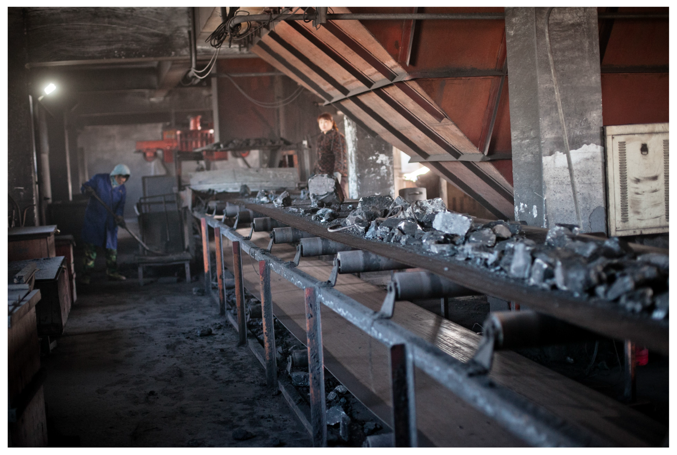
In general, the raw coal is transported to the roll-type crusher to crush coal and gangue to 100 mm after underground mining. Then, spiral size screen machines are applied to screen out materials below 50 mm, limiting the granularity of material within the range 50–100 mm. After that, workers will be standing on both sides of the belt conveyors to remove gangue by hands. Nowadays, the manual selection of gangue is inevitable for most coal mining enterprises in China, although this process is regarded as a labor-intensive job with low efficiency and terrible working environment. In Figure 1, two female workers are standing near the conveyor belts waiting for the upcoming coal and gangue. Moreover, the tedious work is often intolerable with such lighting, air and noise in the coal preparation workshop. Thus, technology for the automatic separation of coal and gangue is severely needed in the coal mining industry.

Currently, the automated separation is performed based on the physical or chemical properties of the various components of raw coal. In view of water use, the methods of coal and gangue separation can be divided into the dry technique or the wet technique [1]. For example, the moving-sieve jigging method and the heavy-medium separation method are the most common wet techniques. Their fundamental principles are very simple, i.e., the different dynamic behaviors of coal and gangue in water. Nonetheless, the enormous maintenance cost and usage of water resources make the wet technique unsuitable for arid regions. Dry techniques apply water-free devices with $\gamma$-rays or X-rays in the existing industrial applications. However, the problems of poor recognition rate and the cumbersome management of radiation sources remain unsolved [3].

Another promising method in recent years to separate coal and gangue is the automated coal–gangue separation system with computer vision, in which industry cameras and computers are used to identify whether the object is coal or gangue through the pattern recognition technology. Ma et al. proposed the coal gangue on-line recognition and automation selection system with digital image processing technology [4]. Zheng et al. studied the pneumatic separation of coal and gangue based on the machine vision system [5]. Figure 2 shows a design of an automated coal–gangue separation system by using the computer vision technology [5,6].

It is worth noting that the computer vision is very similar to the conventional manual separation process of coal and gangue with the development of machine learning (ML) and artificial intelligence (AI). The separation of coal and gangue based on the computer vision method can be divided into the following steps [5]:

• Read digital image obtained from the camera by computers.
• Determine the identification characteristics of coal and gangue.
• Find gangue materials based on the identification algorithms.
• Determine the size and the location of gangue, and then convert these information to the control signals of high pressure air nozzle.

Figure 2 shows a design of an automated coal–gangue separation system by using the computer vision technology [5,6].

In addition, it is interesting to note the feasibility of implementation of image recognition techniques since we could directly modify the current devices from dry techniques by replacing the $\gamma$-rays or X-rays with industrial cameras. Therefore, the use of image recognition to replace the manual separation of coal and gangue has the bright future with advantages of the real-time processing, higher intelligence and lower cost.

However, the recognition rate of the method with computer vision is not satisfactory. Meanwhile, the large computation of the pixel matrices of images brings it low processing speed and poor real-time capability. The challenging task of the feature extraction and classification recognition is looking for the most efficient variables in a great deal of features, which should be distinguishable, reliable, independent and fast. At present, most research is on the grayscale and texture features of coal and gangue via the image recognition method, while the geometric features of their outline curves have not been studied adequately. In reality, because of the distinct hardness of coal and gangue, the edge profiles should be different after the long transportation from underground mining sites. Fracturing in rocks at all scales, from the microscale (microcracks) to the continental scale (megafaults), leads to fractal structures [7]. Many properties such as fragmentation, damage and fracture of rocks, rock burst, joint roughness, rock porosity and permeability, rock gain growth can be described within the concept of fractals in the theory of rock mechanics [8,9]. Therefore, the diverse fractal structures of outline curves of coal and gangue could be reflected and reviewed with the help of fractal and multifractal analysis.

In this paper, we focus on the differences of coal and gangue profiles, trying to utilize the features of multifractality of the outline curve series as the geometric feature to improve the recognition rate with the computer vision technology. The rest of paper is organized as follows: Section 2 gives some preliminary definitions of the stochastic process to the readers with zero knowledge, such as the Hurst parameter, autocorrelation function (ACF), fractal dimensions (FD), self-similar process and long range dependence (LRD) and fractional Brownian motion (fBm). Section 3 and Section 4 introduce and apply the multifractal detrending fluctuation analysis (MFDFA) method, respectively. The recognition methods with results and discussions are given in Section 5. Section 6 concludes the whole article.

2. Preliminaries

2.1. Hurst Parameter, ACF, LRD, FD

When the hydrologist Hurst spent many years analyzing the records of elevation of the Nile River in the 1950s. He found a strange phenomenon: the long-range recording of the elevation time series of the Nile River has much stronger coupling effects [10]. To quantify the level of coupling, the rescaled range (R/S) analysis method was first provided to estimate the coupling level, and Lo modified the original Hurst R/S approach [11]. Later, many useful Hurst parameter estimators were provided and evaluated [12]. However, time series data with trend, seasonality, LRD and multiple scale (multiscaling) behavior cannot be captured by these conventional Hurst methods. A generalization of the Hurst exponent associated with the scaling behavior of statistically significant variables constructed from the time series is proposed in [13].

For a time series $X_t$ ($t=1,2,3,\cdots ,N$), the ACF is defined as follows:

$$\rho \left(k\right)=\frac{Cov(X_t,X_{t-k})}{Var\left(X_t\right)},$$

(1)

where $Cov(·)$ is the covariance and $Var(·)$ is the variance of the series. The behavior of the ACF at $k=0$ determines the local properties of the realizations.

ACF has a close relation with LRD since the asymptotic behavior of ACF at infinity ($k\to \infty$) quantifies the presence or absence of LRD:

$$\rho \left(k\right)\sim c{k}^{-\beta },\mathrm{as}k\to \infty ,$$

(2)

where c is a constant and $\beta \in (0,1)$. LRD also means $\rho \left(k\right)$ is non-integral over the interval $(0,\infty )$. Besides, $\beta$ is related to the Hurst parameter H by using

$$\beta =2-2H.$$

(3)

Therefore, the larger is the H value, the stronger is the LRD or long-range persistence [14]. Specifically, if

$$\rho \left(k\right)\sim 1-{\left|k\right|}^{\alpha },\mathrm{as}k\to 0,$$

(4)

for some $\alpha \in (0,2]$, then the realizations of the random function have the fractal dimension

$$D=n+1-\frac{\alpha }{2}.$$

(5)

The concept of fractals is introduced by Mandelbrot to describe complex systems and phenomena [15]. Generally speaking, the FD of a profile or surface is a roughness measure, with $D\in [n,n+1)$, for a surface in n-dimensional space, with higher values indicating rougher surfaces.

LRDs in time series or spatial data are instead associated with power-law correlations and often referred to as Hurst effects. The Hurst parameter H is a simple parameter which can characterize the level or degree of LRD. If $H=0.5$, the time series has no statistical dependence. If $H<0.5$, the time series is a negatively correlated process or an anti-persistent process. If $H>0.5$, the time series is a positively correlated process [16]. The LRD processes are closely related to fGn and fBm via the fractional calculus. To capture the property of coupling or hyperbolic decaying autocorrelation, fractional calculus based LRD models have been suggested, such as autoregressive fractionally integrated moving average (ARFIMA) model and fractional integrated autoregressive conditional heteroskedasticity (FIGARCH) model [17].

The two quantities D and H are independent of each other: the fractal dimension D is a local property, while LRD index H is a global characteristic. Nevertheless, the two notions are closely linked in much of the scientific literature. This stems from the success of self-similar models such as fractional Gaussian noise and fractional Brownian motion [18]. In addition, the asymptotic relationships Equations (2) and (4) can be expressed equivalently in terms of the spectral density and its behavior at infinity and zero, respectively [19].

2.2. fBm

The fBm with Hurst index $H(0<H<1)$ is defined as the stochastic integral, for $t\ge 0$

$$B_H\left(t\right)=\frac{1}{\Gamma (H+1/2)}\left\{{\int }_{-\infty }^0\left[{(t-s)}^{H-1/2}-{(-s)}^{H-1/2}\right]dW\left(s\right)+{\int }_0^t{(t-s)}^{H-1/2}dW\left(s\right)\right\},$$

(6)

where W denotes a Wiener process defined on $(-\infty ,+\infty )$.

The Hurst parameter H determines the type of fBm and the degree of self-similarity. When $H=0.5$, fBm is reduced to the conventional Brownian motion. The fBm process $B_H\left(t\right)$ has the following covariance function [20]

$$cov(B_H\left(s\right),B_H\left(t\right))=\frac{{\sigma }^2}{2}\left({\left|t\right|}^{2H}+{\left|s\right|}^{2H}+{|t-s|}^{2H}\right).$$

(7)

The mean value of fBm is $E\left(B_H\left(t\right)\right)=0$ and the variance function of fBm is $Var\left[B_H\left(t\right)\right]=\frac{{\sigma }^2}{2}{\left|t\right|}^{2H}$. Figure 3 illustrates 5000 points of fBm and fGn with different Hurst parameters.

The fractional Gaussian noise (fGn) is the increment sequence of fBm. The relationship of white Gaussian noise (wGn) and fBm can be defined with Riemann-Liouville fractional integral [21]:

$$B_H\left(t\right)=\frac{1}{\Gamma (H+1/2)}{\int }_0^t{(t-\tau )}^{H-1/2}\omega \left(\tau \right)d\tau ,$$

(8)

where $H>0$ and $\omega \left(t\right),t>0$ is the one-sided white Gaussian noise.

As discussed above, the constant-order fractional processes with a constant Hurst parameter H can be used to accurately characterize the long memory process and the short-range dependent stochastic processes [22]. However, the multiscaling or multifractal characteristic of stochastic processes cannot be captured by the constant Hurst parameter. Therefore, the multifractional or multifractal processes are the extension of fractional processes by generalizing the constant Hurst parameter H to the case where H is indexed by a time-dependent local Hölder exponent $H\left(t\right)$ with time variant Hurst parameter $H\left(t\right)$ to describe complex or chaotic phenomena in several fields of sciences [23,24]. The performance and the robustness of 12 sliding-windowed Hurst estimators for multifractional processes are reviewed by Sheng et al. [25].

Nonetheless, not all signals are time series, such as the graphic images in geomorphology, urban geography, cartology, etc. Therefore, some novel techniques on fractal image compression and fractal encoding are proposed in [26,27]. In addition, a generalization of the Hurst estimation approach with q-th order moments of the distribution of the increments are used to characterize the statistical evolution of the series in [13]. A process with a constant $H\left(q\right)=H$ shows the characteristic of the monofractal process. For a process with $H\left(q\right)$ depending on the order q, the process is commonly called multi-scaling (or multifractal). In this case, a multifractal spectrum can be defined with the local Hölder exponent quantifies the scaling properties of the process at a given point in time. In Section 3, one of the useful algorithms called multifractal detrending fluctuation analysis (MFDFA) will be introduced to analyze the complex signals which exhibit a local self-similarity property, multifractional processes with variable local Hölder exponent $H\left(q\right)$.

3. MFDFA Algorithm

In the early research studies, many researchers tried to remove the periodicity and trend in a time series to determine the true scale exponents. However, the removal of periodicity inevitably leads to unintended and subjective modification or a smoothing of the fluctuation. This deviation can be overcome by using MFDFA, since the user can choose fitting order m, moment of variances q and scale s. MFDFA is a well-established method to detect multifractality and the scaling behavior of noisy data in the presence of trends with unknown origin and shape.

Detrended fluctuation analysis (DFA) was first proposed by Peng et al. for detecting the long-range correlations of DNA sequences in 1995 [28]. Afterwards, an extension of DFA called multifractal detrending fluctuation analysis (MFDFA) was proposed by Kantelhardt et al. for examining the multifractality of non-stationary time series in 2002 [29]. Currently, MFDFA has been successfully applied to analyze various data, such as hydrographic data [30], wind records [31], financial time series [32], traffic time series [33], control system assessment [34], mechanical vibration signals [35], etc. It has proven to be a powerful tool for uncovering the multifractality of non-stationary time series in the complex systems.

The MFDFA method starts with a possibly non-stationary time series $X_i$ for $i=1,\cdots ,N$, where N indicates its length.

• Transform original data into mean-reduced cumulative sums,

  $$Y_j=\sum _{i=1}^j(X_i-\overline{X}),j=1,\cdots ,N,$$

  (9)

  where $\overline{X}$ is the mean of series, such that the aggregated time series are with zero mean.
• Divide time series $Y_j$ into $N_s=\mathrm{int}(N/s)$ non-overlapping segments of equal length s, starting from the beginning. Since the length N of the series is often not a multiple of the considered time scale s, to not miss any data, another set of segments starting from the end of data is made. As a result, $2N_s$ segments are obtained covering the whole dataset.
• Calculate the local trend for each of the segments $k=1,\cdots ,2N_s$ by a least-square fit of the series.
• Calculate the mean square error $F^2(k,s)$ for the estimate of each segment k of length s.

  $$F^2(k,s)=\frac{1}{s}\sum _{i=1}^s{\left(E[(k-1)s+i]-p_k\left[i\right]\right)}^2,$$

  (10)

  for each segment $k=1,\cdots ,N_s$ and

  $$F^2(k,s)=\frac{1}{s}\sum _{i=1}^s{\left(E[N-(k-N_s)s+i]-p_k\left[i\right]\right)}^2,$$

  (11)

  for each segment $k=N_s+1,\cdots ,2N_s$.
• Average all segments to obtain the qth order variance (or fluctuation) function $F_q\left(s\right)$ for each size s:

  $$F_q\left(s\right)={\left(\frac{1}{2N_s}\sum _{k=1}^{2N_s}{\left[F^2(k,s)\right]}^{q/2}\right)}^{1/q}.$$

  (12)

  For $q=0$ use

  $$F_0\left(s\right)=\exp \left\{\frac{1}{4N_s}\sum _{k=1}^{2N_s}\ln \left(F^2(k,s)\right)\right\},$$

  (13)
• Repeat Steps (2)–(5) for different s evaluating new sets of variances $F_q\left(s\right)$.
• Plot $F_q\left(s\right)$ for each q in log–log scale and estimate the linear fit with least squares. If slope $h\left(q\right)$ varies with q, multifractality is suspected. Single slope shows monofractal scaling.
• Calculate multifractal exponent $t\left(q\right)$ as

  $$t\left(q\right)=qh\left(q\right)-1.$$

  (14)
• Use Legendre transform to evaluate the q-order singularity–Hölder exponent $h\left(q\right)$ and corresponding dimension $D\left(q\right)$:

  $$\left\{\begin{array}{c}h\left(q\right)=dt\left(q\right)/dq\\ D\left(q\right)=qh\left(q\right)-t\left(q\right)\end{array}\right.$$

  (15)

For the above steps of calculation methodology, Ihlen developed the MATLAB code in [36]. The approach is used to calculate multifractal spectrum, with graph log($F_q$) versus log(s) identifying crossovers with different q orders.

The slope $H_q$ of scaling function $F_q$ with different q order demonstrates the LRD behavior of signals. The multifractal spectrum indicates how much dominant are the various fractal exponents present in the series. Therefore, the width of the singularity spectrum $\Delta \left(h_q\right)$ = max($h_q$) − min($h_q$) is often used to quantitatively measure the degree of multifractality in the series, that is, wider spectra indicate more multifractality.

4. Applying MFDFA to the Outline of Coal and Gangue

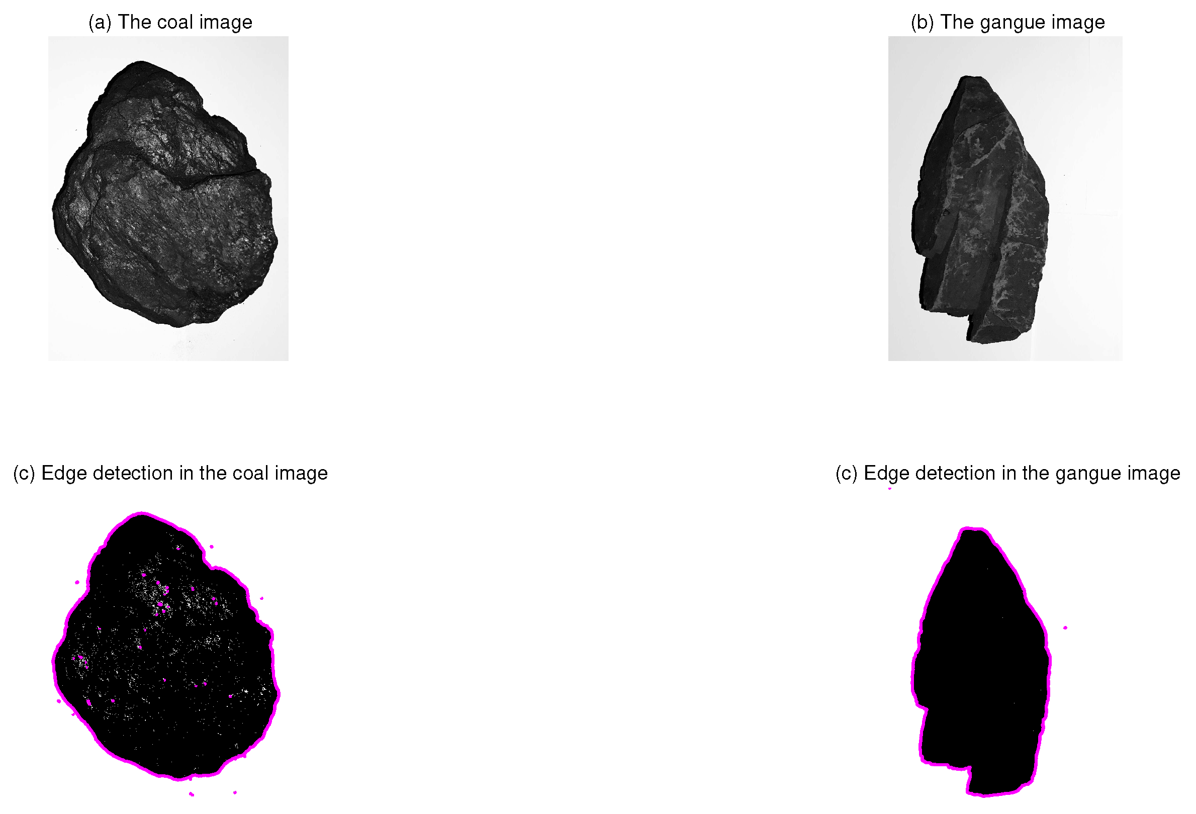
The sampled images of coal and gangue are compressed and binarized to detect edges. As shown in Figure 4, the identified edges of coal and gangue are highlighted with magenta curves. Even though some irrelevant scattered points are detected, it is not difficult to identify the outline curve series from the detected edges.

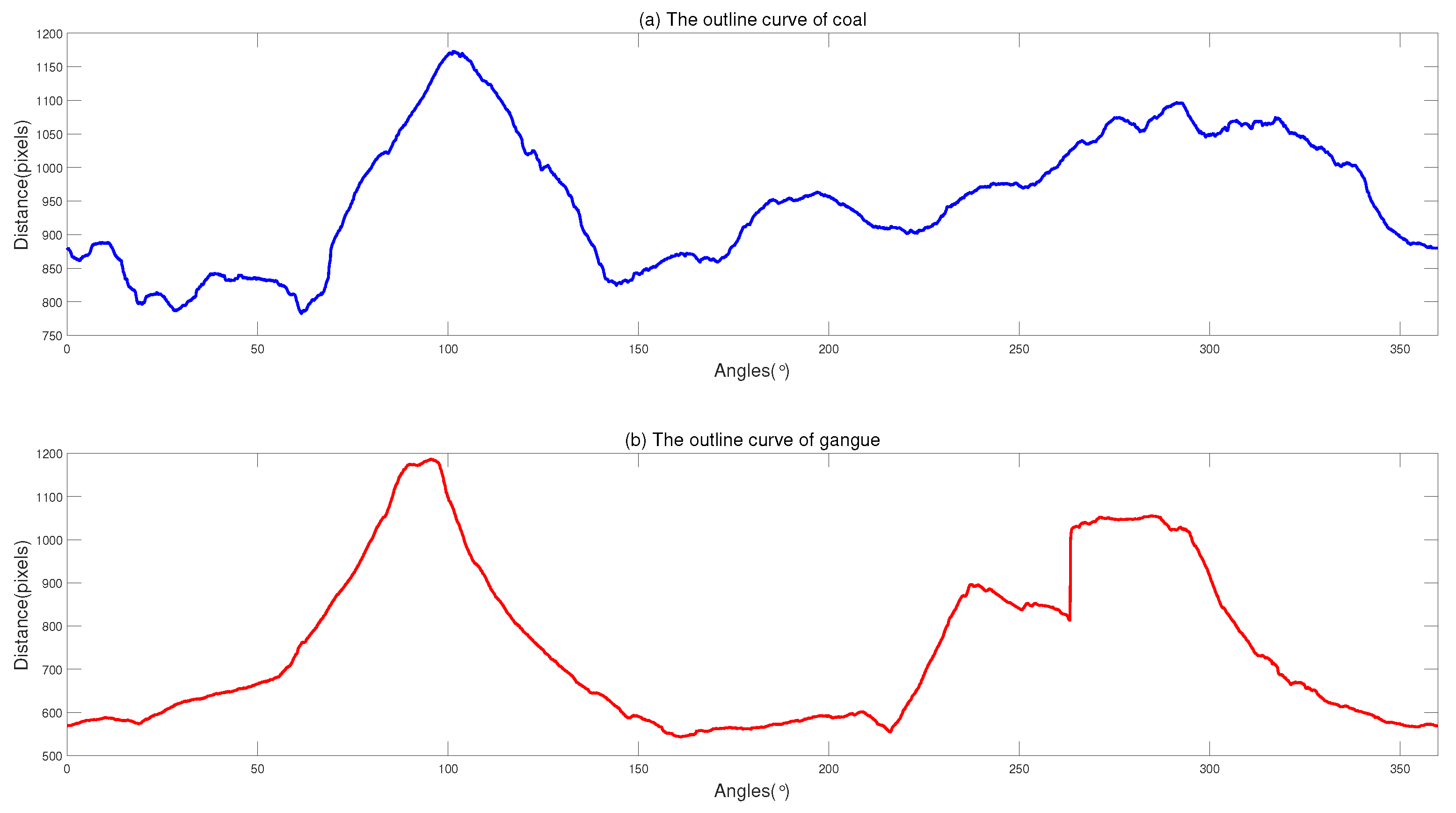
The identified edges are carried out and transformed into the polar coordinates from the center at the accuracy of 0.1 degrees. The random walk series of the outline curves of coal and gangue can be obtained accordingly with 3600 points in Figure 5.

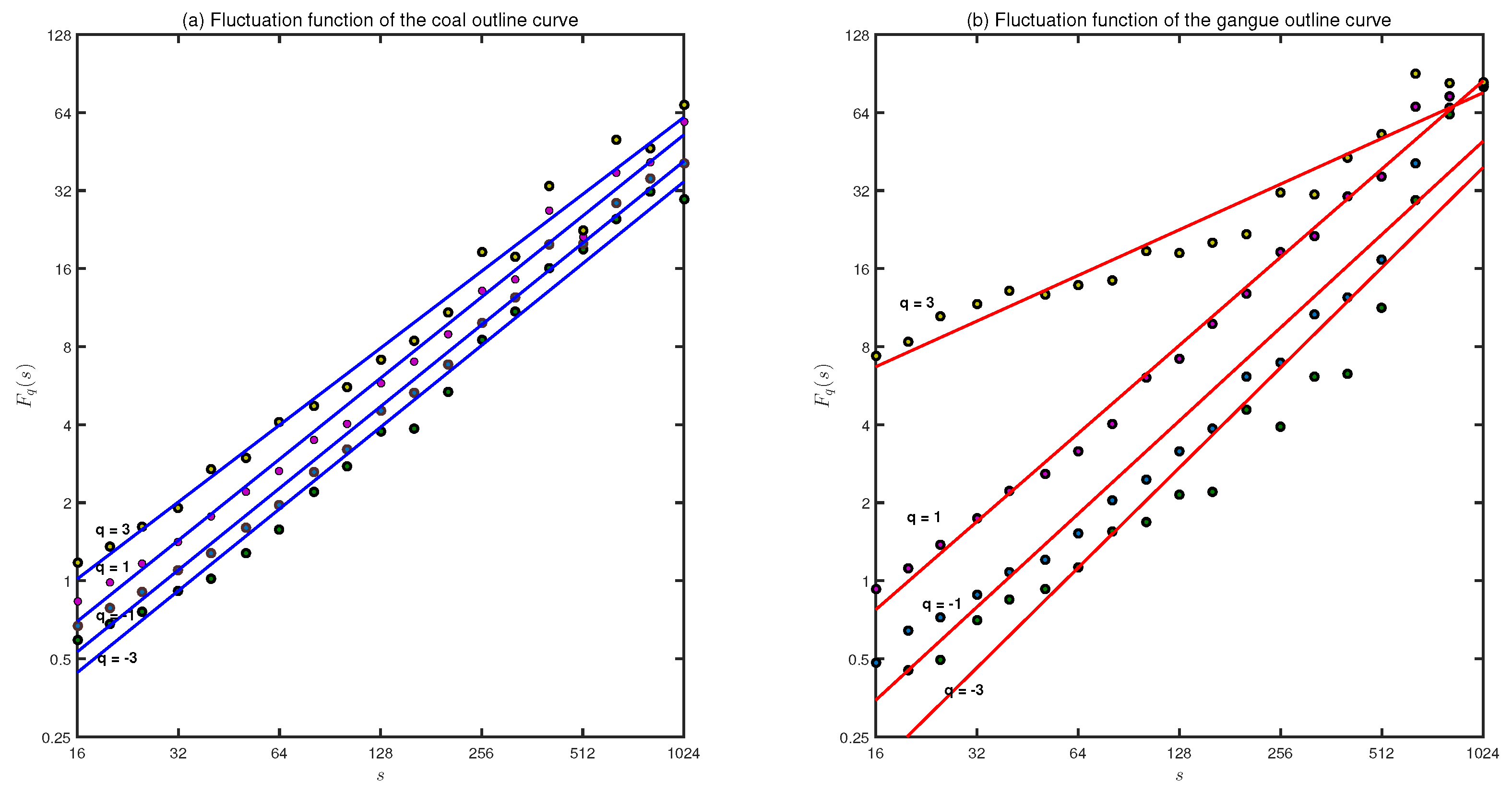
According to the MFDFA algorithm introduced in Section 3, the MFDFA fluctuation functions $F_q\left(s\right)$ for the outline curves of coal and gangue are shown versus the scale s in a log–log plot with q = $-3$, $-1$, 1, 3 in Figure 6. The q-order generalized Hurst parameter can now be defined and viewed as the slopes $H_q$ of regression lines for each q-order fluctuation function $F_q\left(s\right)$. The contrasting q dependence of the gangue outline curve compared with that of coal can clearly be seen in Figure 6.

The q-order generalized Hurst parameter can now be defined and viewed as the slopes $H_q$ of regression lines for each q-order fluctuation function $F_q\left(s\right)$. The contrasting q dependence of the gangue outline curve compared with that of coal can clearly be seen.

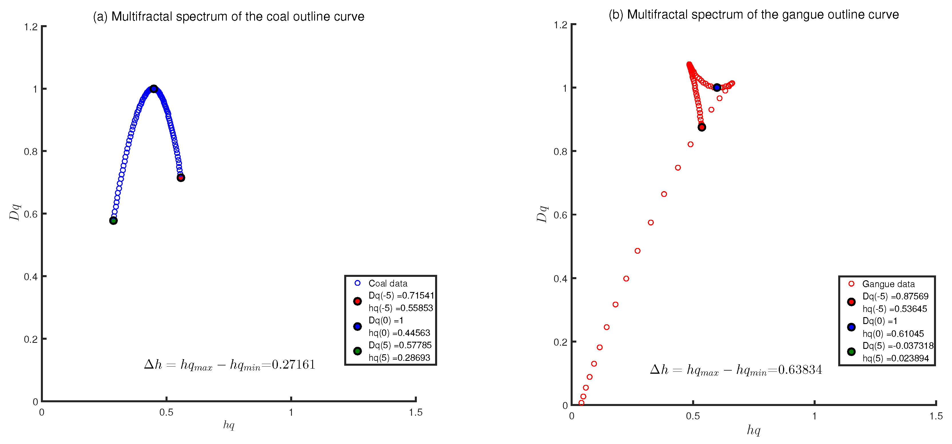
Next, the multifractal spectrum of the outline curves of coal and gangue can be obtained (Figure 7).

The origin of multifractality of a time series can be distinguished as two different types, i.e., the multifractality due to: (i) the different long-range correlations of the number fluctuations; and (ii) the broadness of probability density function (PDF) of the distributions [29].

The easiest way to eliminate the correlations for (i) is shuffling the original series into random order, since the multifractality is due to the probability density, which is not affected by the shuffling procedure. For (ii), the surrogate process of data, defined as replacing the phase of discrete Fourier transform (DFT) coefficients of the original data with a set of pseudo independent and identically distributed quantities in $(-\pi ,pi)$, can change the broad PDF of the original data into the Gaussian distribution and seldom destroys the intrinsic long-range correlations of the original data [29].

$$F_q\left(s\right)/F^{shuf}\left(s\right)\sim s^{h\left(q\right)-h_{shuf}\left(q\right)}=s^{h_{corr\left(q\right)}}$$

(16)

$$F_q\left(s\right)/F^{surr}\left(s\right)\sim s^{h\left(q\right)-h_{surr}\left(q\right)}=s^{h_{PDF\left(q\right)}}$$

(17)

where $H_{shuf}\left(q\right)$ is the generalized Hurst parameter of the shuffled data, $H_{corr}\left(q\right)$ is the generalized Hurst exponent of the only long-range correlation data, $H_{surr}\left(q\right)$ denotes the generalized Hurst parameter of the surrogate data, and $H_{PDF}\left(q\right)$ indicates the generalized Hurst exponent of the only broad PDF data. If only the fat PDF causes the multifractality of time series, then $H\left(q\right)=H_{shuf}\left(q\right)$ and $H_{corr}\left(q\right)=0$. Conversely, if only the long-range correlations occur in time series, then $H_{shuf}\left(q\right)=0.5$. Additionally, if two types of multifractality exist together, both $H_{shuf}\left(q\right)$ and $H_{surr}\left(q\right)$ will depend on q.

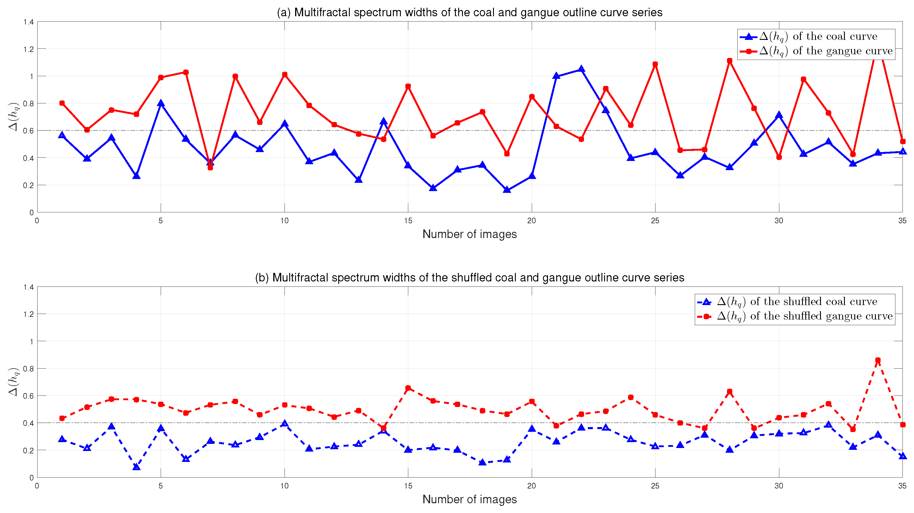
To remove the long-range correlations of the series, the original series of coal and gangue curves are shuffled and re-calculated with MFDFA in Figure 8. Consequently, the multifractal spectrums become narrower after the removal of the LRD correlations.

Without loss of generality, more series of coal and gangue outline curves are plotted in Figure 9, and the outliers of $\Delta h$ at 5, 21, 22, 23, and 30 in Figure 9a are modified after the series are shuffled. A clear threshold value at 0.4 is marked with dot dash line in Figure 9b. However, no such confident line can be drawn in Figure 9a since the two types of multifractality are affecting the multifractal features of coal and gangue outline curve series. Therefore, in this paper, the shuffled data with $\Delta \left(h_q\right)$ are used as the geometric characteristics of the coal and gangue outline curves.

5. Pattern Recognition Methods and Discussions

To start with, the performance of the proposed method is validated by applying it to distinguish different types of outline curves from coal and gangue. The results may be different when using different pattern recognition and classification methods. Several artificial neural networks (ANN), such as back propagation (BP) neural network, radial basis function kernel (RBF) neural network, and k nearest neighbor (kNN), are applied in the pattern recognition for classification and regression.

BP neural network is a kind of supervised learning method usually applied for the classification task, the goal of which is to find a function that best maps a set of inputs to their correct output. Replacing the activation function with the Gaussian RBF kernel is the RBF neural network, which is another method commonly used in practice. The k-NN algorithm is a type of instance-based learning, or lazy learning, which is fastest and simplest of all machine learning algorithms. More introductions of pattern recognition and machine learning algorithms can be referred in [37,38].

5.1. Grayscale and Texture Features of the Image

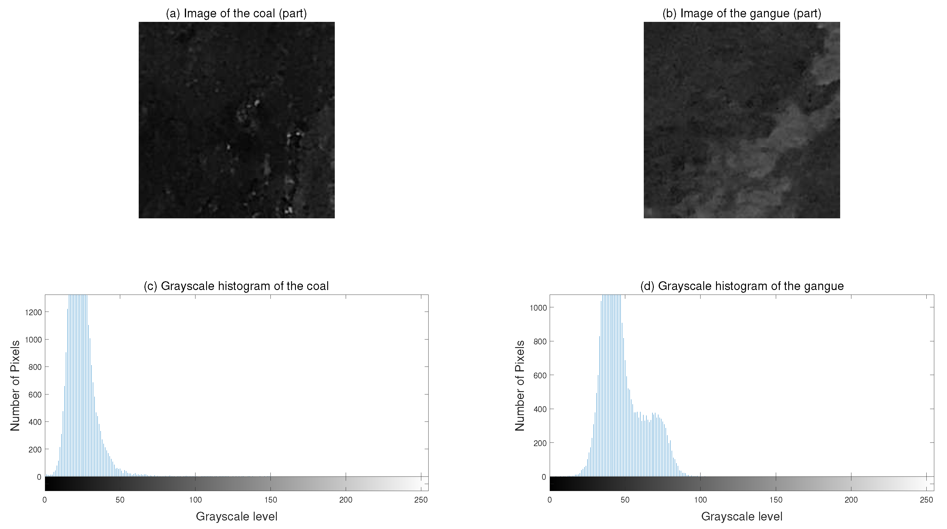
Grayscale histogram is a type of histogram that indicates the number of pixels for each grayscale value in the whole image. Some statistical variables can be calculated accordingly such as average, variance, smoothness, skewness, entropy, etc. [6]. It is proven to be an efficient and simple way in identifying coal and gangue [39]. Figure 10 shows the grayscale histogram of coal and gangue. The co-occurrence matrix is used to quantify the numerical features based on the spatial arrangement of the selected region.

Meanwhile, it should be noted that there are nine variables or arguments in grayscale histogram and co-occurrence matrix in the feature extraction process [6], which will take too much computer memory leading to the dimension disaster. To solve the emerging problem, excluding insignificant arguments and picking identical ones can speed up the recognition process. Therefore, the average of the grayscale histogram is chosen as one of the notable grayscale features to be extracted based on the chemical properties of coal and gangue. Besides, the second-order moment of the co-occurrence matrix is used to represent the texture features of the image to help coal–gangue identification.

In our study, more than 500 sampled figures are used for the training of BP, RBF, and kNN neural networks, and 50 sets of new figures are imported as the test data. The corresponding recognition rates are summarized in

Table 1. Comparison of the recognition rate with different methods.

Features Used in Pattern Recognition	BP	RBF	kNN
Grayscale features [40,41]	65.0%	47.5%	67.5%
Texture features	47.5%	62.5%	65.0%
Grayscale and texture features [4,42]	62.5%	60.0%	90.0%
Grayscale, texture and geometric features	72.5%	70.0%	97.5%

. The proposed method with grayscale, texture and geometric features can achieve a recognition rate of 97.5%.

5.2. Discussions

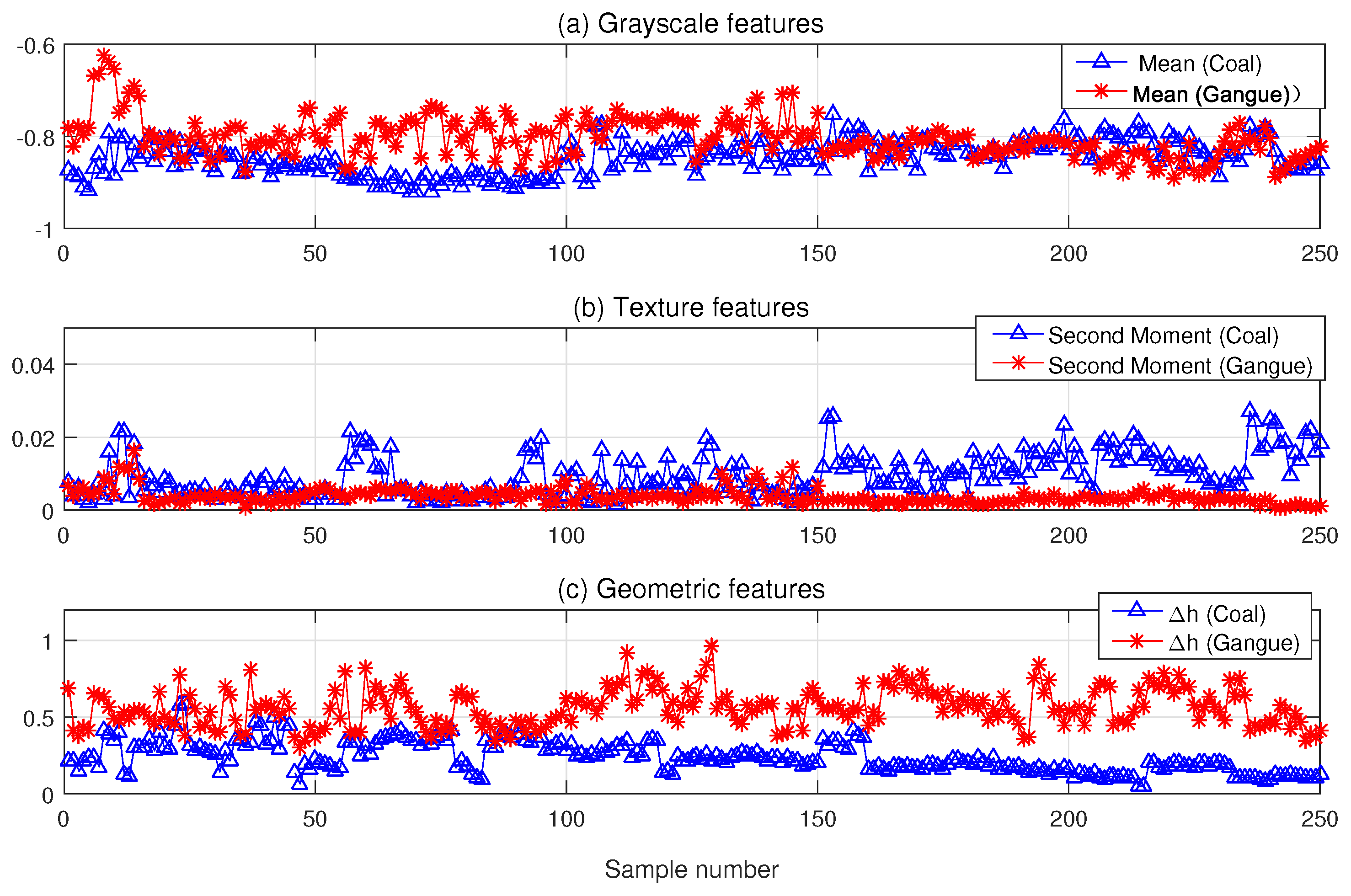
Here, we give some possible reasons the proposed method can give good performance in the recognition of coal and gangue. In practice, it is usually essential to cut a square in the middle of the image to guarantee the smooth calculation of the pixel matrices when extracting grayscale and texture features, such as Figure 10a,b. However, the particle size of coal and gangue could be so various that picking a relatively small square of the whole image may be misleading. Hence, the geometric feature contains a new dimension of the information, which contributes to the higher recognition rate of the proposed method without losing the overall information of the coal and gangue image. Furthermore, its geometric features are not correlated (coupled) with the other two arguments. All grayscale, texture and geometric feature variables are summarized in Figure 11.

6. Conclusions

In this paper, we propose a novel method for the feature extraction of coal and gangue using computer vision technology. The MFDFA method is applied to extract the geometric features of coal and gangue in view of different multifractal structures in the outline curves of coal and gangue. Besides, the MFDFA algorithm with shuffling operations is used to modify the singularity width $\Delta h$ as the geometric feature variables. Various pattern recognition methods such as BP neural network, RBF neural network, k-NN algorithm are selected to compare the recognition efficiency. Test results show that the proposed geometric features combined with grayscale and texture features can achieve a recognition rate of 97.5%.

References

- Gui, X.; Liu, J.; Cao, Y.; Miao, Z.; Li, S.; Xing, Y.; Wang, D. Coal preparation technology: Status and development in China. Energy Environ. 2015, 26, 997–1013. [Google Scholar] [CrossRef]
- Zhang, J.X.; Miao, X.X. Underground disposal of waste in coal mine. J. China Univ. Mining Technol. 2006, 35, 197–200. [Google Scholar]
- Qi, X.; Yongchuan, Z. A novel automated separator based on dual energy gamma-rays transmission. Meas. Sci. Technol. 2000, 11, 1383. [Google Scholar] [CrossRef]
- Ma, X.M.; Song, X.R. Coal gangue online recognition and automation selection system based on ARM and CAN bus. In Proceedings of the 2005 International Conference on Machine Learning and Cybernetics, Guangzhou, China, 18–21 August 2005; Volume 2, pp. 988–992. [Google Scholar]
- Zheng, K.; Du, C.; Li, J.; Qiu, B.; Yang, D. Underground pneumatic separation of coal and gangue with large size (≥50 mm) in green mining based on the machine vision system. Powder Technol. 2015, 278, 223–233. [Google Scholar] [CrossRef]
- Hou, W. Identification of coal and gangue by feed-forward neural network based on data analysis. Int. J. Coal Prep. Util. 2017, 1–11. [Google Scholar] [CrossRef]
- Xie, H. Fractals in Rock Mechanics; CRC Press: Boca Raton, FL, USA, 1993. [Google Scholar]
- Xie, H.; Sun, H.; Ju, Y.; Feng, Z. Study on generation of rock fracture surfaces by using fractal interpolation. Int. J. Solids Struct. 2001, 38, 5765–5787. [Google Scholar] [CrossRef]
- Ju, Y.; Sudak, L.; Xie, H. Study on stress wave propagation in fractured rocks with fractal joint surfaces. Int. J. Solids Struct. 2007, 44, 4256–4271. [Google Scholar] [CrossRef]
- Hurst, H.E. Long-term storage capacity of reservoirs. Trans. Am. Soc. Civil Eng. 1951, 116, 770–808. [Google Scholar]
- Lo, A.W. Long-Term Memory in Stock Market Prices; Technical report; National Bureau of Economic Research: Cambridge, MA, USA, 1989. [Google Scholar]
- Ye, X.; Xia, X.; Zhang, J.; Chen, Y. Effects of trends and seasonalities on robustness of the Hurst parameter estimators. IET Signal Process. 2012, 6, 849–856. [Google Scholar] [CrossRef]
- Di Matteo, T. Multi-scaling in finance. Quantit. Financ. 2007, 7, 21–36. [Google Scholar] [CrossRef]
- Li, M. Record length requirement of long-range dependent teletraffic. Phys. A Stat. Mech. Appl. 2017, 472, 164–187. [Google Scholar] [CrossRef]
- Mandelbrot, B.B. Fractals; Wiley Online Library: Hoboken, NJ, USA, 1977. [Google Scholar]
- Kale, M.; Butar, F.B. Fractal analysis of time series and distribution properties of Hurst exponent. J. Math. Sci. Math. Educ. 2011, 5, 8–19. [Google Scholar]
- Liu, K.; Chen, Y.; Zhang, X. An Evaluation of ARFIMA (Autoregressive Fractional Integral Moving Average) Programs. Axioms 2017, 6, 16. [Google Scholar] [CrossRef]
- Mandelbrot, B.B.; Van Ness, J.W. Fractional Brownian motions, fractional noises and applications. SIAM Rev. 1968, 10, 422–437. [Google Scholar] [CrossRef]
- Clegg, R.G. A practical guide to measuring the Hurst parameter. Mathematics 2005, 6, 43–55. [Google Scholar]
- Li, M.; Chi, C.H. A correlation-based computational model for synthesizing long-range dependent data. J. Frankl. Inst. 2003, 340, 503–514. [Google Scholar] [CrossRef]
- Sheng, H.; Chen, Y.; Qiu, T. Fractional Processes and Fractional-Order Signal Processing: Techniques and Applications; Springer Science & Business Media: New York, NY, USA, 2011. [Google Scholar]
- Peltier, R.F.; Véhel, J.L. Multifractional Brownian Motion: Definition and Preliminary Results. Ph.D. Thesis, INRIA, Cedex, France, 1995. [Google Scholar]
- Muniandy, S.; Lim, S. Modeling of locally self-similar processes using multifractional Brownian motion of Riemann-Liouville type. Phys. Rev. E 2001, 63, 046104. [Google Scholar] [CrossRef] [PubMed]
- Liu, S.; Lu, M.; Liu, G.; Pan, Z. A novel distance metric: Generalized relative entropy. Entropy 2017, 19, 269. [Google Scholar] [CrossRef]
- Sheng, H.; Chen, Y.; Qiu, T. Tracking performance and robustness analysis of Hurst estimators for multifractional processes. IET Signal Process. 2012, 6, 213–226. [Google Scholar] [CrossRef]
- Liu, S.; Pan, Z.; Song, H. Digital image watermarking method based on DCT and fractal encoding. IET Image Process. 2017, 11, 815–821. [Google Scholar] [CrossRef]
- Liu, S.; Pan, Z.; Cheng, X. A novel fast fractal image compression method based on distance clustering in high dimensional sphere surface. Fractals 2017, 25, 1740004. [Google Scholar] [CrossRef]
- Peng, C.K.; Havlin, S.; Stanley, H.E.; Goldberger, A.L. Quantification of scaling exponents and crossover phenomena in nonstationary heartbeat time series. Chaos Int. J. Nonlinear Sci. 1995, 5, 82–87. [Google Scholar] [CrossRef] [PubMed]
- Kantelhardt, J.W.; Zschiegner, S.A.; Koscielny-Bunde, E.; Havlin, S.; Bunde, A.; Stanley, H.E. Multifractal detrended fluctuation analysis of nonstationary time series. Phys. A Stat. Mech. Appl. 2002, 316, 87–114. [Google Scholar] [CrossRef]
- Zhang, Q.; Xu, C.Y.; Chen, Y.D.; Yu, Z. Multifractal detrended fluctuation analysis of streamflow series of the Yangtze River basin, China. Hydrol. Process. 2008, 22, 4997–5003. [Google Scholar] [CrossRef]
- Telesca, L.; Lovallo, M. Analysis of the time dynamics in wind records by means of multifractal detrended fluctuation analysis and the Fisher–Shannon information plane. J. Stat. Mech. Theory Exp. 2011, 2011, P07001. [Google Scholar] [CrossRef]
- Wang, Y.; Wei, Y.; Wu, C. Analysis of the efficiency and multifractality of gold markets based on multifractal detrended fluctuation analysis. Phys. A Stat. Mech. Appl. 2011, 390, 817–827. [Google Scholar] [CrossRef]
- Shang, P.; Lu, Y.; Kamae, S. Detecting long-range correlations of traffic time series with multifractal detrended fluctuation analysis. Chaos Solitons Fractals 2008, 36, 82–90. [Google Scholar] [CrossRef]
- Domański, P.D. Multifractal Properties of Process Control Variables. Int. J. Bifurc. Chaos 2017, 27, 23. [Google Scholar] [CrossRef]
- Lin, J.; Chen, Q. Fault diagnosis of rolling bearings based on multifractal detrended fluctuation analysis and Mahalanobis distance criterion. Mech. Syst. Signal Process. 2013, 38, 515–533. [Google Scholar] [CrossRef]
- Ihlen, E.A.F.E. Introduction to multifractal detrended fluctuation analysis in Matlab. Front. physiol. 2012, 3, 141. [Google Scholar] [CrossRef] [PubMed]
- Duda, R.O.; Hart, P.E.; Stork, D.G. Pattern Classification; John Wiley & Sons: New York, NY, USA, 2012. [Google Scholar]
- Nasrabadi, N.M. Pattern recognition and machine learning. J. Electron. Imaging 2007, 16, 049901. [Google Scholar]
- Li, W.; Wang, Y.; Fu, B.; Lin, Y. Coal and coal gangue separation based on computer vision. In Proceedings of the Fifth IEEE International Conference on Frontier of Computer Science and Technology (FCST), Changchun, China, 18–22 August 2010; pp. 467–472. [Google Scholar]
- Wang, R.; Liang, Z. Automatic separation system of coal gangue based on DSP and digital image processing. In Proceedings of the IEEE Symposium on Photonics and Optoelectronics (SOPO), Wuhan, China, 16–18 May 2011; pp. 1–3. [Google Scholar]
- Tripathy, D.; Reddy, K.G.R. Multispectral and joint colour-texture feature extraction for ore-gangue separation. Pattern Recognit. Image Anal. 2017, 27, 338–348. [Google Scholar] [CrossRef]
- Liang, H.; Cheng, H.; Ma, T.; Pang, Z.; Zhong, Y. Identification of coal and gangue by self-organizing competitive neural network and SVM. In Proceedings of the 2nd IEEE International Conference on Intelligent Human-Machine Systems and Cybernetics (IHMSC), Nanjing, China, 26–28 August 2010; Volume 2, pp. 41–45. [Google Scholar]
Figure 1.
Manual separation of coal and gangue.
Figure 2.
The automated coal–gangue separation system with computer vision. PLC: Programmable Logic Controller, LED: Light Emitting Diode.
Figure 3.
Fractional Brownian motion (fBm) and fractional Gaussian noise (fGn). In the left panel, from top to bottom, are fBm with H = 0.5, 0.6, 0.7, and 0.8. In the right panel, from top to bottom, are fGn with H = 0.5, 0.6, 0.7, and 0.8. With the increase of Hurst exponent H, the coupling effects of fBm and fGn are strengthened.
Figure 4.
Images of: coal (a); and gangue (b). Edge detections of: coal (c); and gangue (d). The identified edges of coal and gangue are highlighted with magenta curves.
Figure 5.
Outline curves of: coal (a); and gangue (b). The identified edges are carried out and transformed into the polar coordinates from the center at the accuracy of 0.1 degrees.
Figure 6.
Fluctuation functions of the outline curves for: (a) coal; and (b) gangue. The q-order generalized Hurst parameter can now be defined and viewed as the slopes of regression lines for each q-order fluctuation function . The contrasting q dependence of the (a) coal outline curve compared with that of (b) gangue can clearly be seen in the above figure.
Figure 7.
Multifractal spectrum of: (a) coal and (b) gangue outline curve series. The width of the multifractal spectrum is defined as .
Figure 8.
Multifractal spectrum of the shuffled (a) coal and (b) gangue outline curve series. The multifractal spectrums become narrower after the removal of the long-range correlations.
Figure 9.
Spectrum widths of: (a) the original coal and gangue curve series; and (b) the shuffled series. A clear threshold value at 0.4 is marked with dot dash line in (b) while no such confident line can be drawn in (a).
Figure 10.
Images of: (a) coal; and (b) gangue; and grayscale histograms of: (c) coal; and (d) gangue respectively.
Figure 11.
(a) Grayscale features of coal and gangue; (b) Texture features of coal and gangue; (c) Geometric features of coal and gangue.
© 2018 by the authors. Licensee MDPI, Basel, Switzerland. This article is an open access article distributed under the terms and conditions of the Creative Commons Attribution (CC BY) license (http://creativecommons.org/licenses/by/4.0/).
Share and Cite
MDPI and ACS Style
Liu, K.; Zhang, X.; Chen, Y. Extraction of Coal and Gangue Geometric Features with Multifractal Detrending Fluctuation Analysis. Appl. Sci. 2018, 8, 463. https://doi.org/10.3390/app8030463
AMA Style
Liu K, Zhang X, Chen Y. Extraction of Coal and Gangue Geometric Features with Multifractal Detrending Fluctuation Analysis. Applied Sciences. 2018; 8(3):463. https://doi.org/10.3390/app8030463
Chicago/Turabian StyleLiu, Kai, Xi Zhang, and YangQuan Chen. 2018. "Extraction of Coal and Gangue Geometric Features with Multifractal Detrending Fluctuation Analysis" Applied Sciences 8, no. 3: 463. https://doi.org/10.3390/app8030463
Note that from the first issue of 2016, this journal uses article numbers instead of page numbers. See further details here.