A Hydrodynamic Modelling Framework for Strangford Lough Part 1: Tidal Model

Abstract

Hydrodynamic models are a powerful tool that can be used by a wide range of end users to assist in predicting the effects of both physical and biological processes on local environmental conditions. This paper describes the development of a tidal model for Strangford Lough, Northern Ireland, a body of water renowned for the location of the first grid-connected tidal turbine, SeaGen, as well as the UK’s third Marine Nature Reserve. Using MIKE 21 modelling software, the development, calibration and performance of the model are described in detail. Strangford Lough has a complex flow pattern with high flows through the Narrows (~3.5 m/s) linking the main body of the Lough to the Irish Sea and intricate flow patterns around the numerous islands. With the aid of good quality tidal and current data obtained throughout the Lough during the model development, the surface elevation and current magnitude between the observed and numerical model were almost identical with model skill >0.98 and >0.84 respectively. The applicability of the model is such that it can be used as an important tool for the prediction of important ecological processes as well as engineering applications within Strangford Lough.

1. Introduction

Hydrodynamic models of bays and estuaries have traditionally been used for coastal engineering applications including the design of development projects such as breakwaters and harbours, sediment transport processes and water quality. More recently their application has been utilized by the marine energy industry to determine optimal sites for exploitation of marine energy converters (MEC) [1], as well as in the development of tools to enable MEC farm layouts to be optimised for maximum energy extraction [2,3]. Hydrodynamic models are also increasingly being used to couple hydrodynamics with ecological processes such as larval dispersal [4,5,6] and to provide closer insight into conservation and water quality concerns [7]. However for hydrodynamic models to be effective there is a fundamental requirement that they are calibrated and validated properly [8,9].

The development, calibration and validation of a numerical physical model that covers an extensive area characterised by a complex hydrography can be difficult. Many adjustments may be required to be made to the bathymetry and grid resolution before a model can be used with certainty to investigate a study [9,10]. A further consideration is the validity of the field data, the model will only be as good as the field data with which it is calibrated. To accurately simulate the entire domain of a complex system is difficult [10] and it is often found that a high correlation is attained in certain areas of the model domain but at a cost of weaker correlation in other areas.

The study area presented here comprises a series of complex hydrodynamic aspects, being the combination of a narrow tidal inlet with a relatively large scale basin attached. High tidal ranges at the entrance and large storage inside the basin give rise to strong flows and a multitude of islands and rocky outcrops add to considerable complexity in the flow patterns. This highly energetic environment has resulted in considerable interest to be harnessed for power generation. Since 2008 Strangford Lough has been home to the world’s first large scale, grid-connected tidal stream generator, SeaGen which has a rated output of up to 1.2 MW of electricity for on average 10 h each tidal cycle. SeaGen is located in the Strangford Narrows, a narrow channel approximately 8 km long, on average 30 m deep and 0.5 km wide at the narrowest part linking the main body of Strangford Lough to the Irish Sea. At its inner end, the channel opens out abruptly into Strangford Lough, the largest inlet in the British Isles covering 134 km² of water and characterised by more than 100 islands, numerous pladdies (intertidal reefs) and large areas of intertidal mudflats [11]. Complex flow patterns exists within the Lough ranging from extremely high flows through the Narrows (~3.5 m/s) to intricate flow patterns around the islands and pladdies [11]. The flow constriction associated with the Narrows gives rise to a tidal phase shift of ~105 min over 10 km from the Irish Sea to the southern end of Lough. The high tidal current velocities in the Narrows, together with the close proximity to the shore and grid-connection, have made the location a highly attractive site for tidal turbine testing. Owing to the major interest in the Strangford Narrows as a test-site for full-size and scaled tidal turbines, it was necessary to develop a well-calibrated and effective hydrodynamic model in the Narrows.

In addition to Strangford Lough being of major interest for the testing of tidal energy devices, it is also an area with high conservation status. The Lough which is designated as the UK’s third Marine Nature Reserve and is listed as a NATURA 2000 area (UK0016618) [12] has also been identified as a pilot Marine Protected Area (MPA) [13] because of the presence of biogenic reefs of the horse mussel Modiolus modiolus [14,15]. As a Special Area of Conservation (SAC), focus has now shifted to restoration of Strangford Lough shellfish reefs including M. modiolus and the native oyster (Ostrea edulis) for both subtidal and intertidal populations. There is also a growing focus in the Lough in experimentally farming macroalgae for biofuel which requires the knowledge of water motion around the plants. With these designations and interests, there is considerable pressure from regulatory authorities and ecologists for the development of predictive models relating to processes such as larval and spore dispersal of organisms and mammal carcass movement. Such models clearly require a solid hydrodynamic basis and this consideration also provided considerable stimulus for the development of the model described below.

The paper presents a detailed hydrodynamic model simulating tidal flow of Strangford Lough (Figure 1) sufficiently accurate to predict ecological processes throughout the entire domain from the high flows in the Narrows to the complex flow areas in the main area of the Lough. The model is versatile such that it provides a platform which can be utilized by numerous end users including engineers and ecologists and to show that hydrodynamic models have the potential to be valuable tools for environmental management of ecologically important areas.

Figure 1. Location of Strangford Lough in Northern Ireland and the Strangford Lough model domain.

Figure 1. Location of Strangford Lough in Northern Ireland and the Strangford Lough model domain.

2. Methods

2.1. General Hydrodynamic Model Setup Description

MIKE 21 Flow model flexible mesh (FM) uses a finite volume method to determine the current field by solving a depth integrated incompressible Reynolds averaged Navier-Stokes equation. Calculations are performed in each cell using a cell-centered finite volume method. Higher order time integration and space discretization was chosen for the shallow water equations with a critical CFL (Courant-Friedrich-Lévy) of 0.7. Since maximum tidal elevation inside and outside the Lough can reach ~4 m, the flood and dry facility was included using the standard program settings (0.005 m drying depth; 0.05 flooding depth; 0.1 m wetting depth). The barotropic mode was selected for density so that both salinity and temperature were held constant during the simulation as salinity is nearly uniform and constant in Strangford Lough [16]. Temperature only varies by 6 °C between winter and summer (Figure 2) and tends to be well mixed vertically over large parts of the Lough. The Smagorinsky formulation was selected for the eddy viscosity which was held constant throughout the domain with a value of 0.28 [17]. The range of flow rates in Strangford Lough reflect the complex range of substrata types in the Lough ranging from soft featureless sediment in areas with low flows through to harder substrates as current increases throughout the model domain [18]. The depth of the Lough can range from −70 to 0 m. In the absence of detailed information on spatially varying bed roughness a Manning-Strickler number M of 36 m^(1/3)/s (equivalent to Manning’s n of 0.028 s/m^1/3) was specified for the bed resistance in the final model version. In the calibration process several attempts were made to capture the difference in roughness in certain parts of the Narrows and areas of the Lough as known from dive surveys or marked on the navigation chart. In all cases, however, this showed a decrease in performance of the model compared to the observed elevations and currents and thus a fixed friction value was employed throughout the domain. The Coriolis forcing was set to vary within the domain although the effect was negligible given the small size of the domain. Wind forcing, ice coverage, tidal potential, precipitation, evaporation, wave radiation or any form of structures (including SeaGen) were not included in the simulation.

Figure 2. Observed seawater temperature (°C) from June 2011 to December 2012 obtained from the Portaferry Quay Aqualogger 520PT.

Figure 2. Observed seawater temperature (°C) from June 2011 to December 2012 obtained from the Portaferry Quay Aqualogger 520PT.

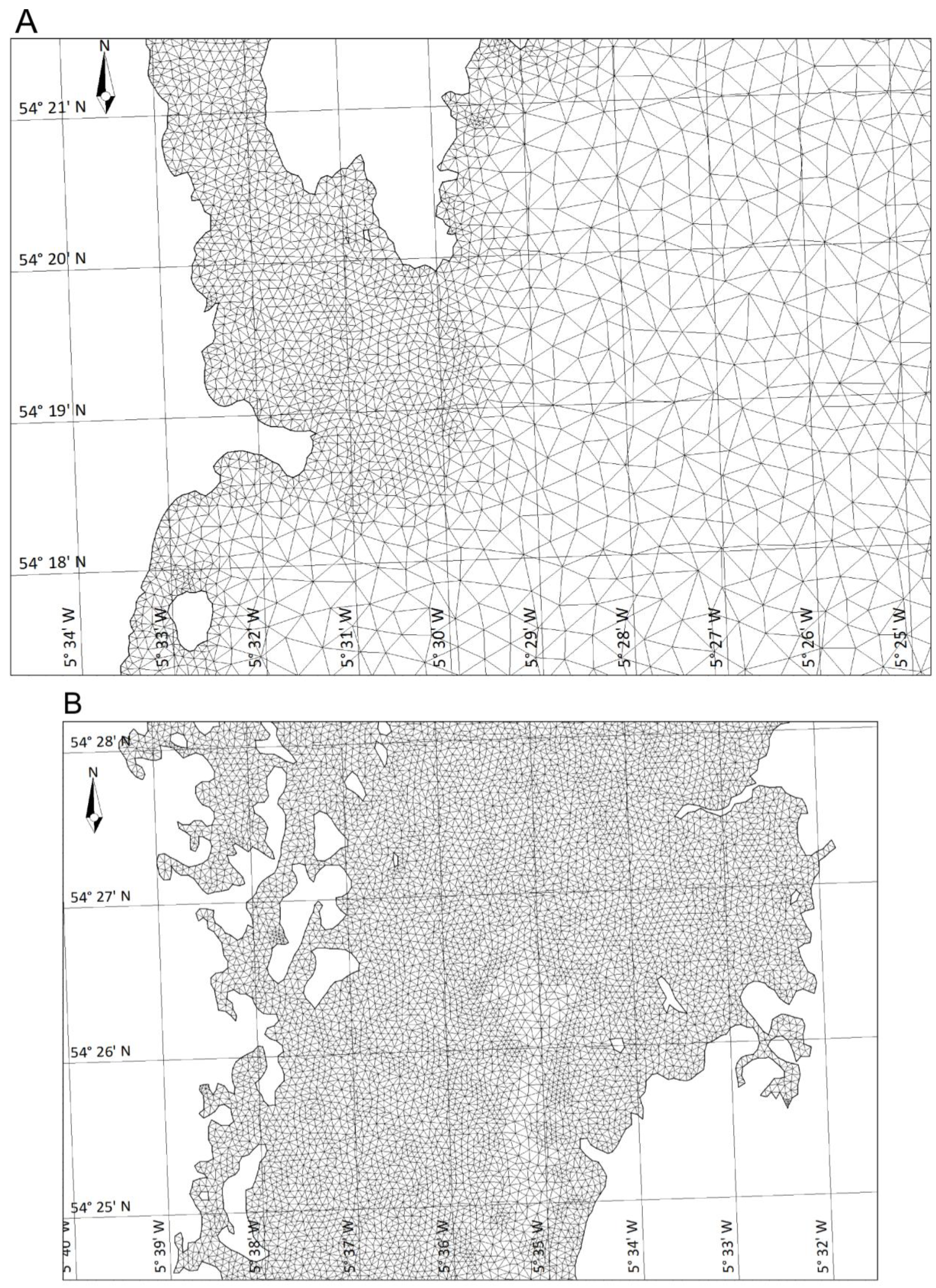
2.2. Model Area, Mesh and Mesh Detail

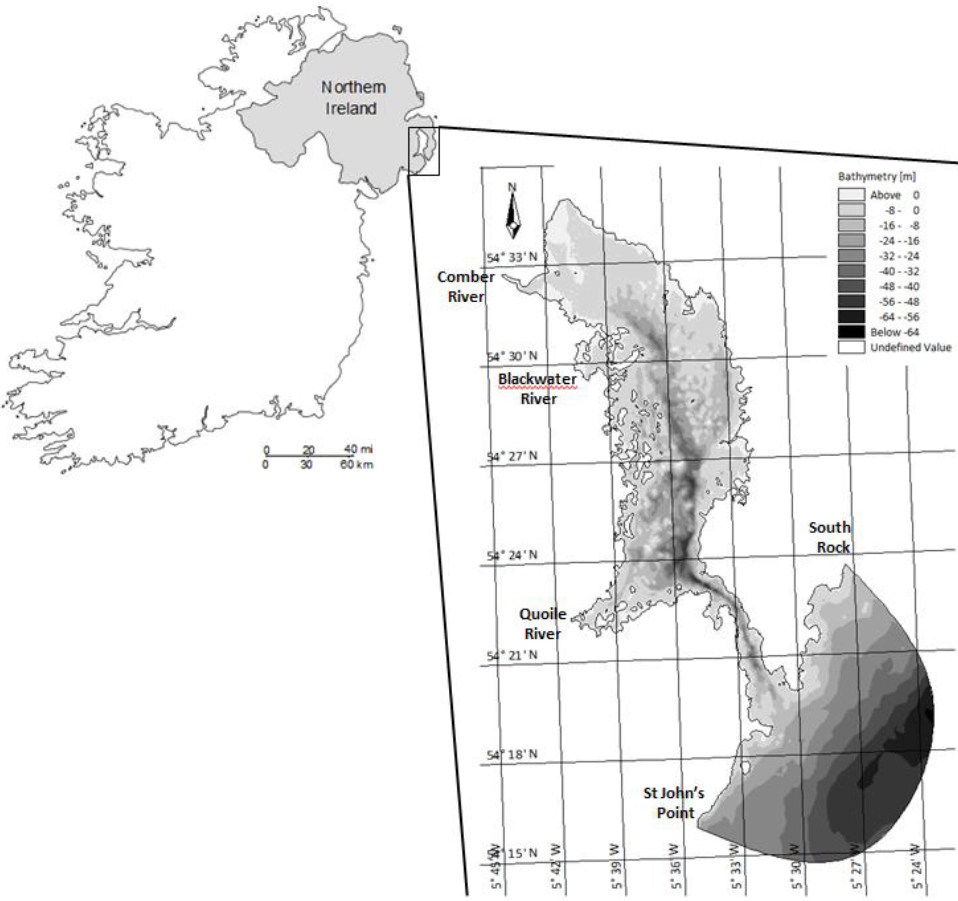
The model area includes the Strangford Lough in Northern Ireland and part of the Irish Sea from South Rock in the North (N 54°24′, W −5°27′) to St John’s Point in the South (N 54°16′, W −5°36′) (Figure 1). These two points are joined in an arc taking the seaward open boundary sufficiently far from the high velocity outflows of the Strangford Narrows. In the calibration of the model this was identified as an issue with the original boundary being much closer to the Narrows than in the final model. The mesh can be constructed using either quadrangular or triangular elements or both using a flexible mesh (FM) technology [19]. In this application triangular element cells were used only to build the model allowing the user to define the size of the computational cells which may vary depending on the area of interest. Cell size will determine the accuracy of results from the model simulations to real time data so that the smaller the cell size, the more precise the model will be, but at the expense of computational speed. Outside Strangford Lough the cell size averaged ~200 m (Figure 3A), whereas within the Narrows and the inlets, the primary areas of interest, cell size averaged ~50 m (Figure 3B). This mesh resolution resulted in a total of 52,882 cells and 28,041 nodes in the final model version presented here (Strngf_6V05_msl).

Figure 3. Detailed mesh of the entrance to Strangford Lough (A) and inside Strangford Lough, characterised by islands and pladdies (B).

Figure 3. Detailed mesh of the entrance to Strangford Lough (A) and inside Strangford Lough, characterised by islands and pladdies (B).

2.3. Bathymetry

The bathymetry information was obtained from two sources. Part of the data was derived from SeaZone Raster bathymetry data referenced to chart datum. While the SeaZone data is offered as a seamless gridded data set, in this instance it was found to be deficient in the intertidal and shallow water area. Furthermore part of the Comber River inlet is missing in the digital data set. Thus intertidal heights were supplemented using data from the Admiralty chart 2156 Strangford Lough (December 2007 edition). Once a complete data set was obtained the datum was corrected to mean sea level using a corrective surface derived from lowest astronomical tide (LAT) to mean sea level differences.

2.4. Boundary Conditions

Strangford Lough is almost land-locked with a landward catchment area of 647 km² [20]. This area is relatively small considering the total Lough area of 134 km² such that salinity is nearly uniform and constant throughout the year [16]. The immediate surrounding area is relatively flat with most areas below 30 m elevation above sea level but with a maximum elevation of 290 m above sea level to the North of the Lough [20]. The total fresh water inflows are estimated at 495 mm per annum based on hydrological modelling (320 × 10⁶ m³/year, on average 10 m³/s) with relatively slow response (time to peak in the order of hours) to rainfall events [20]. There are three major freshwater inflow points; the Comber River in the northwest, the Blackwater River in the west and the Quoile River in the south west (Figure 1), the latter being barraged to allow inflows at certain stages of the tide only. The remaining runoff enters the Lough through direct runoff or small streams of mostly less than 5 km stream length.

The model has been designed with three open boundaries, one coastal and two fluvial boundaries, plus the capability of adding precipitation and direct runoff if needed. The catchment area of the Comber River is 62.6 km², the Blackwater 50.1 km² while the Quoile River is 244.3 km² representing 9%, 7% and 37% of the total Lough catchment respectively [20]. The freshwater inputs into the Lough are considered insignificant in terms of the overall contribution to tidal heights and flow rates and have been designated as zero discharge boundaries in this instance. However the fluvial boundaries can be reinstated if studies require these boundaries for example in the context of water quality aspects or studies on localised stratification of freshwater. As a result of the considerations only one open boundary was applied in the model: that is the open-sea boundary located outside Strangford Lough.

Figure 4. Map of Strangford Lough showing the locations of pressure sensors and current meters used to obtain surface elevation and current data. Location of discharge reference line used to calculate the total water flux is also included.

Figure 4. Map of Strangford Lough showing the locations of pressure sensors and current meters used to obtain surface elevation and current data. Location of discharge reference line used to calculate the total water flux is also included.

To calibrate the model a time series of surface elevation was required at this boundary. Initially boundary condition data were obtained from the Irish Tide and Storm Surge Model (ITSSM) [21]. However during 2011 tide gauge data were obtained at either end of the open-sea boundary (South Bay and Guns Island; Figure 4); these data were of suitable quality to obtain diurnal and semidiurnal harmonics for prediction of tidal elevations at these locations. Data from both sites obtained from April to July 2011 showed that the tidal elevation and phasing were almost identical (Figure 5). Therefore it was deemed that a spatially uniform surface elevation was sufficient to force the oscillation in water levels and currents within the Strangford Lough Model. For the calibration and subsequent operation of the model (see below), predicted astronomic tidal elevation from South Bay provided a higher quality prediction due to a slightly longer tide sensor deployment period than at Guns Island. In addition the ITSSM can be used to supplement the predicted astronomic elevations with seasonal (monthly and annual) components as well as storm surge residuals for inundation and extreme water level estimates.

Figure 5. Comparison of South Bay and Guns Island surface elevation data obtained in May 2011.

Figure 5. Comparison of South Bay and Guns Island surface elevation data obtained in May 2011.

2.5. Field Data for Calibration and Validation of the Model

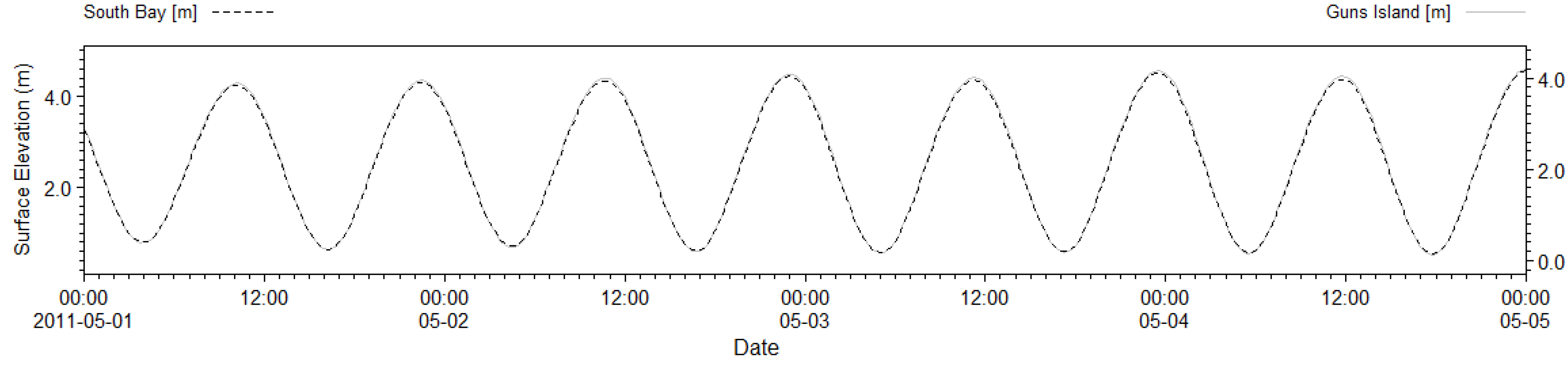
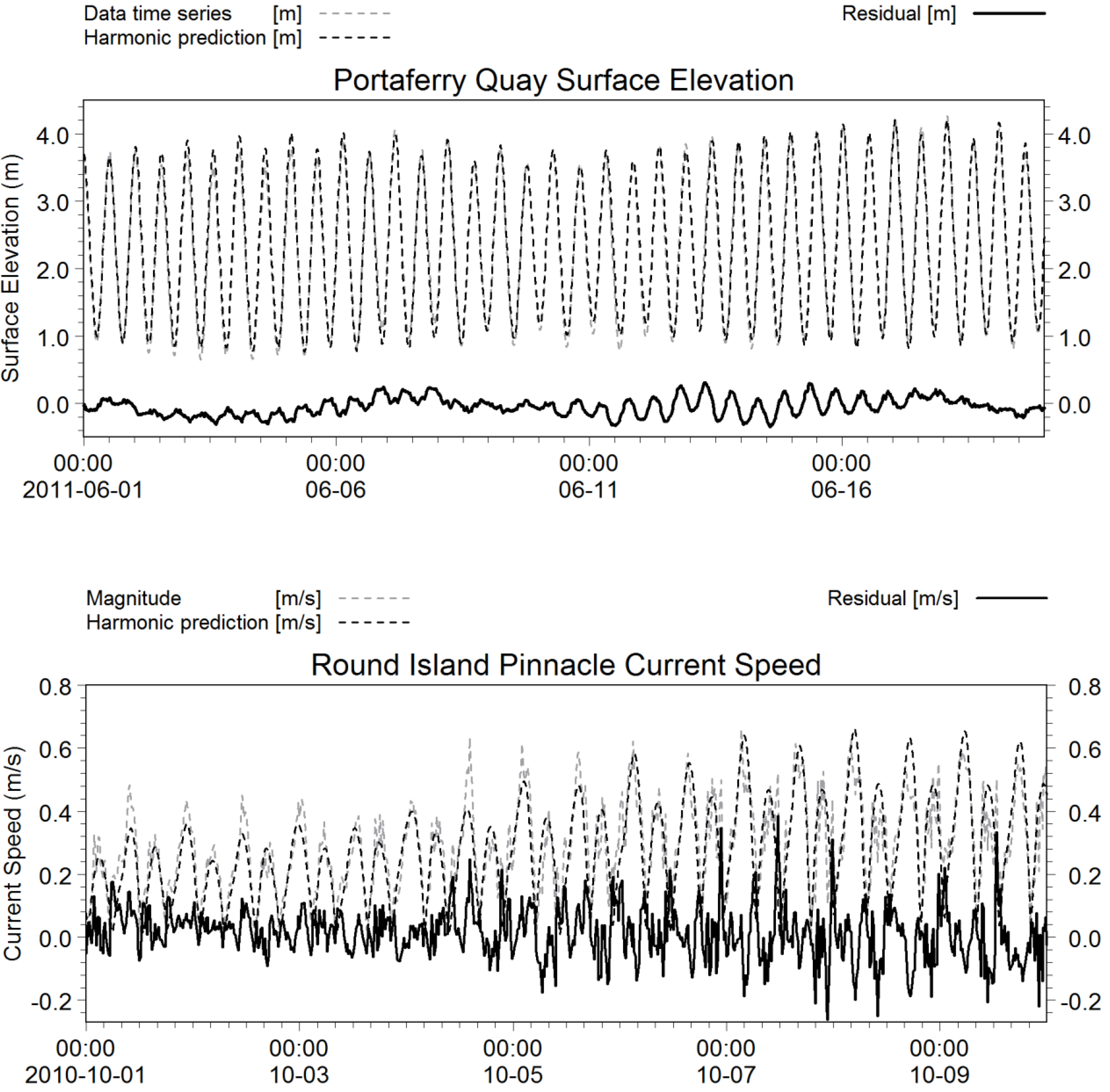
2.5.1. Tidal Elevation Data Collection and Harmonic Analysis

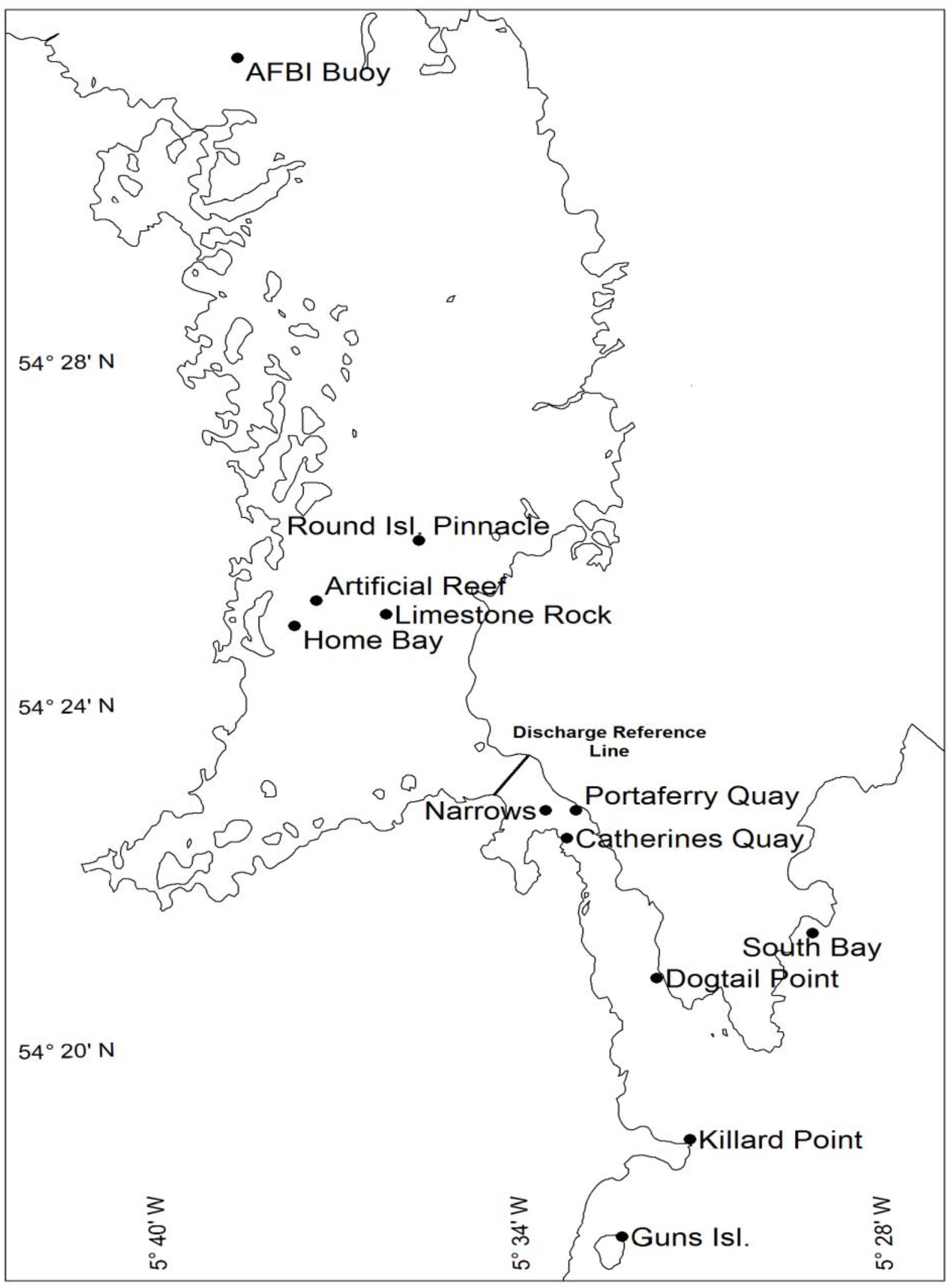
While Strangford Lough has been of considerable interest for some time in terms of tidal patterns and ecology, relatively limited high quality tidal data were readily available at the start of this model development. Tidal prediction data available from the UK Hydrographics Office for Strangford Quays appear to be based on a relatively short record dating some years back [22]. Therefore during 2010–2012 considerable field data were collated from a total of seven mobile tide gauge deployments in the study area (Table 1; Figure 4). Instruments used were pressure transducers logging subsea pressure and temperature (Aqualogger 520PT, Aquatec Group, Hampshire, RG27 8NY, UK). Pressure data were collected at 15 min intervals using the average from 128 s, 1 Hz sample bursts. All pressure data obtained were first quality checked for any anomalies (e.g., spikes, gaps) and then corrected for changes in atmospheric pressure during the monitoring period. Data for this pressure correction was obtained from an atmospheric pressure sensor (OM-CP-PRTEMP110, Omega Engineering Ltd., Manchester, M44 5BD, UK) located at the Queen’s University Marine Laboratory (QML), which was cross checked with pressure data from the local weather station [23]. Tidal analyses utilising the IOS method [24] were carried out by means of the Matlab toolbox T-Tide [25] to derive the standard and shallow water tidal constituents. These constituents were then used to predict the tidal heights either with MIKE 21 Tidal Prediction of Heights toolbox or T-Tide.

Table 1. Location (in Easting and Northing to Irish National Grid), type (surface elevation or current) and length of time (days or months) that data were collected for the calibration of the Strangford Lough hydrodynamic model.

Location	Easting	Northing	Length	Data Type
Killard Point	361,147 m	343,597 m	3 months	surface elevation
Dogtail Point	360,550 m	347,075 m	3 months	surface elevation
Portaferry Quay	359,100 m	350,700 m	4 months	surface elevation
Catherines Quay	358,939 m	350,092 m	3 months	surface elevation
Limestone Rock	355,695 m	354,924 m	3 months	surface elevation
Home Bay	354,042 m	354,672 m	3.5 months	surface elevation
AFBI Buoy	353,025 m	366,910 m	3.5 months	surface elevation
AFBI Buoy	353,025 m	366,910 m	16 days	current speed
Round Island Pinnacle	356,284 m	356,510 m	28 days	current speed
Artificial Reef	354,436 m	355,213 m	14 days	current speed
Narrows	350,692 m	358,558 m	3 months	current speed

Table 1. Location (in Easting and Northing to Irish National Grid), type (surface elevation or current) and length of time (days or months) that data were collected for the calibration of the Strangford Lough hydrodynamic model.

Location	Easting	Northing	Length	Data Type
Killard Point	361,147 m	343,597 m	3 months	surface elevation
Dogtail Point	360,550 m	347,075 m	3 months	surface elevation
Portaferry Quay	359,100 m	350,700 m	4 months	surface elevation
Catherines Quay	358,939 m	350,092 m	3 months	surface elevation
Limestone Rock	355,695 m	354,924 m	3 months	surface elevation
Home Bay	354,042 m	354,672 m	3.5 months	surface elevation
AFBI Buoy	353,025 m	366,910 m	3.5 months	surface elevation
AFBI Buoy	353,025 m	366,910 m	16 days	current speed
Round Island Pinnacle	356,284 m	356,510 m	28 days	current speed
Artificial Reef	354,436 m	355,213 m	14 days	current speed
Narrows	350,692 m	358,558 m	3 months	current speed

2.5.2. Current Data Collection and Harmonic Analysis

For the calibration of the Strangford Lough model, current data were obtained from three different deployments of SonTek/YSI ADP instruments (Table 1). Initially current data were also obtained from an ADP deployment from within the Narrows however the data were unreliable and thus not used. To validate the model in the Narrows, a SonTek/YSI ADP instrument was deployed at Church Point within the Narrows for a three month period (Table 1). Current measurements were derived from 2 min time averaged samples with pings at 1Hz transformed to velocity vectors in the coordinate system East, North, Up relative to magnetic north. The internal compass was compensated with the instrument installed in the relevant deployment frame. Velocities were gathered at 15 min intervals in 1 m vertical bins extending from ~0.7 m above the seabed to the surface. The data were first processed by removing erroneous values near the surface due to sidelobe interference using the instantaneous water depth and thereafter filtered using a low-bandpass with passband of 2.08 × 10⁻⁴ Hz and stopband of 2.77 × 10⁻⁴ Hz. Depth averaged velocity (DAV) was derived taking account of missing data due to blanking distance and sidelobe interference. Harmonic analysis and current prediction were derived using the MIKE 21 toolbox for tidal analyses and prediction of currents for the AFBI Buoy, Round Island Pinnacle and Artificial Reef ADP deployments only. Data collected from the Narrows ADP deployment were only processed for erroneous values and filtered as noted above.

2.6. Model Calibration

Flows in Strangford Lough are dominated by astronomic tides of semidiurnal nature, with probably in excess of 90% of the movement being controlled by this process. To support this observation the surface elevation and current velocities are compared against the harmonic prediction. The residual elevation and velocities give an indication of both the quality of the harmonic prediction and any non-harmonic components caused for example by meteorological effects. Thus tidal and current predictions were derived for the same time period of the longest time series measured. For one surface elevation site (Portaferry Quay) and one current measurement site (Round Island Pinnacle) the residual was determined as outlined above. The comparison of measured and predicted surface elevation is shown in Figure 6 together with the residual for a representative subset of the data. Small influences of meteorological effects can be observed in the gradually varying residual for surface elevation, as well as some deficits in the harmonic prediction (shorter period oscillation in the order of one tidal cycle). It can be clearly seen that overall the surface elevation and current velocity are dominated by astronomic effects (Figure 6). As outlined in the introduction the model calibration and validation will therefore focus on the hydrodynamics caused by astronomic tides.

Figure 6. Comparison of measured data and harmonically predicted data with residual for one surface elevation site (Portaferry Quay) and one current speed site (Round Island Pinnacle).

Figure 6. Comparison of measured data and harmonically predicted data with residual for one surface elevation site (Portaferry Quay) and one current speed site (Round Island Pinnacle).

Calibration of the Strangford Lough model was undertaken using a range of tidal elevation data sets and current data based on seven sites for the tidal elevation and three sites for current flows (see Table 1). The spread in site locations ensured a range in phases and current flows to enable us to modify the model to ensure a good overall data fit throughout the Lough. Initial checking and correction of the bathymetry was required as there were several instances where the height of the pladdies was not accurate; corrections were made based on the Admiralty chart data for Strangford Lough. Further modifications of the model were carried out by either altering the eddy viscosity or bed resistance values.

The calibration was carried out over a 15 day period in October including the warm-up of the model. The warm-up period was of the order of one tidal cycle, though in the analysis the first 24 h were excluded, such that the total period calibrated incorporated one neap and one spring period. Generally, calibration periods would be over a larger duration, in particular if the resonance of the basin to be modeled is in the order of any of the semidiurnal components driving the model. In this instance this is not the case with the basin wave period in the order of 40 min. Therefore as a calibration period a set of neap and spring tidal cycles was selected, this includes tidal ranges in excess of a mean spring cycle to less than a mean neap cycle. Thus a large range of tidal velocities is being modeled in a short period of time resulting in a wide mix of conditions to be assessed in the calibration, reducing runtime and amount of data to be processed. Hence the response of the basin over a longer period becomes largely dependent on the quality of the boundary condition if the model responds well to the forcing provided in the shortened calibration period.

Figure 7. Comparison of surface elevation between the harmonically predicted and numerical model at: Portaferry Quay, Limestone Rock and the AFBI buoy during the period 1–14 October 2010.

Figure 7. Comparison of surface elevation between the harmonically predicted and numerical model at: Portaferry Quay, Limestone Rock and the AFBI buoy during the period 1–14 October 2010.

The surface elevation obtained from the numerical model was comparable to that of the harmonically predicted data from the seven locations used for the calibration of the surface elevation (only three representative sites shown; Figure 7). At all locations a similar pattern was observed between the model and harmonically predicted period. During the spring high level tides, the model slightly over-predicted surface elevation. In contrast there was a slight under-prediction by the model compared to the predicted harmonic data during the neap low levels (Figure 7). Phasing between the model and harmonic predictions were almost identical for each site.

Observations of current speed derived from the model were also strongly comparable to that of the harmonically predicted data at the three sites (Figure 8). The pattern of higher velocities on the flood tide and lower velocities on the ebb tide were simulated by the model for all the sites, but to varying degrees of precision. For the AFBI buoy site, the model was slightly over-predicting throughout the calibration period compared to the Round Island Pinnacle site where the model was slightly under-predicting (Figure 8). Although current speeds between the model and predicted data were similar, for the Artificial Reef site there was a slight delay in the time taken for the model to reach slack low water.

Figure 8. Comparison of current speed between the harmonically predicted and numerical model at: AFBI Buoy, Artificial Reef and Round Island Pinnacle during the period 5–10 October 2010.

Figure 8. Comparison of current speed between the harmonically predicted and numerical model at: AFBI Buoy, Artificial Reef and Round Island Pinnacle during the period 5–10 October 2010.

3. Results

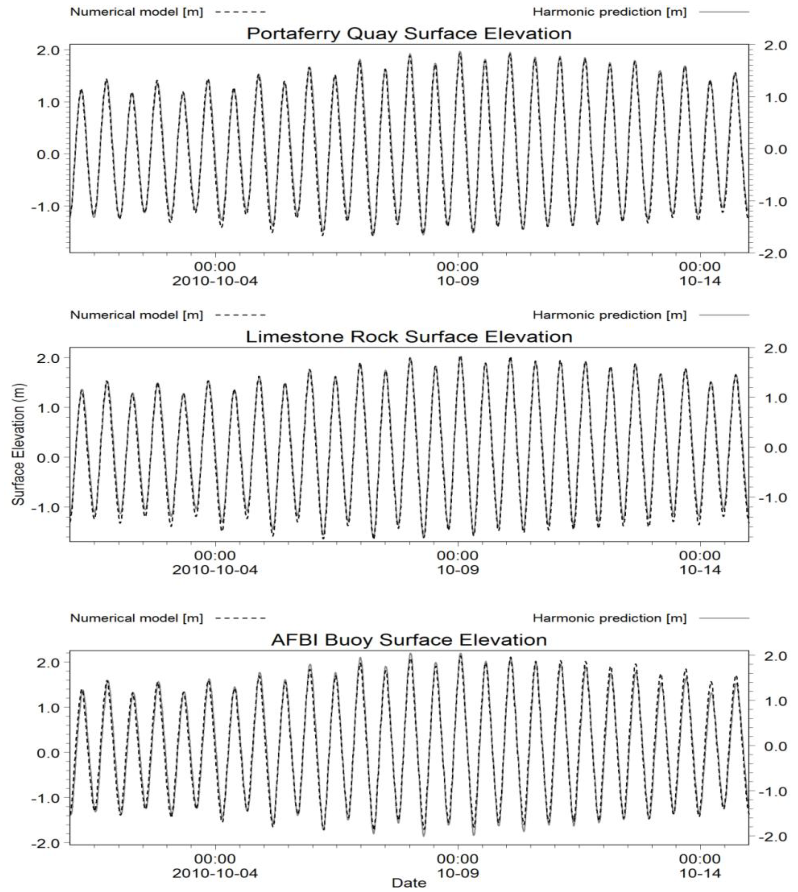
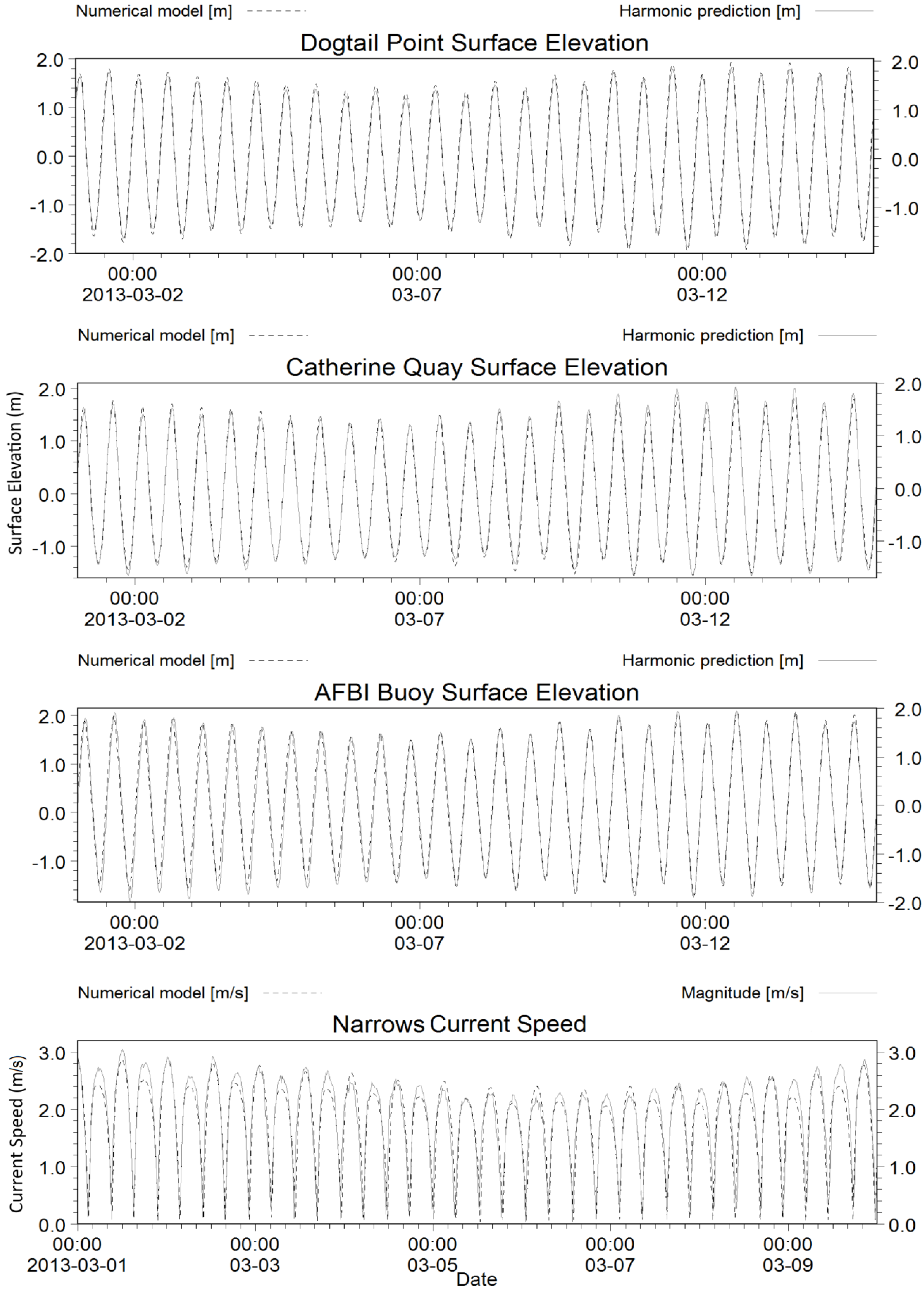
3.1. Model Validation

To demonstrate that the model is capable of making accurate predictions for periods outside the calibration period, the model was run using the same setup, mesh and open boundary conditions as for the calibration model during the period 1–31 March 2013. The surface elevations at the seven sites together with current flows at the four sites throughout the domain were used for the validation exercise to show the accuracy and predictive capability of the model. Details on the harmonic components used to predict the tidal elevations and current velocities are given in Table 2. It can be seen that the number of harmonics used varies depending on the length of the data record and the complexity of the tide at the given location [26]. This means however that the model accuracy may also be underestimated at a given location if the representation by the tidal harmonic prediction is of lower quality.

To evaluate and quantify the quality of the agreement between the model predictions and observations several quantitative metrics were used to capture different aspects of model performance: the modelling efficiency (MEF) as per definition by Stow et al. [27], skill as per definition by Dias and Lopes [9], root mean square (RMS), and bias. The MEF measures how well a model predicts (modelled minus observed) relative to the average observations with values close to one considered excellent. Similarly the skill value provides a quantitative assessment between the predicted and observed values, with stronger emphasis on the observed mean. Skill tends to give a higher agreement in tidal elevation assessment, since the mean of the observation should be zero if referenced to mean seas level. In both instances, values higher than 0.95 are considered an excellent agreement between the model and predictions. Bias and RMS measure the size of the difference between predicted and observed values (in the same units as the measure), where RMS gives stronger weight to individual samples with large differences (for example during spring tides). Both goodness-of-fit parameters should be as small as possible.

In all instances the model output closely fits the harmonically predicted surface elevation data (Table 3; Figure 9). MEF and Skill values are very close to unity, revealing an excellent agreement between the model and harmonically predicted surface elevation data. RMS values ranged from 0.04 m to 0.14 m between model and predicted surface elevation, less than 5% of the local tidal range. Bias was on average 17% smaller for surface elevation. The agreement between the modelled and predicted/observed current data is of less agreement compared to the surface elevation as is often found, though overall agreement for the model skill was still high except for the artificial reef site [21]. The comparison here focuses on the current magnitude, since in general directions were within the accuracy of the internal compass readings of the ADCPs. Round Island Pinnacle and the Narrows site give a high goodness-of-fit for skill and relatively low bias and RMS values given the total current magnitudes (~10% of maximum current magnitude). The AFBI buoy site has a lower skill and MEF, but bias and RMS are still around 10%, artificial reef shows a poorer correlation with bias and RMS close to 20% of the maximum current magnitude. However Figure 6 shows some discrepancy already at calibration stage at this location.

Table 2. List of harmonic constituents used in predicting surface elevation at Killard Point (KP), Dogtail Point (DP), Portaferry Quay (PQ), Catherines Quay (CQ), Limestone Rock (LR), Home Bay (HB), AFBI Buoy (AB) and in predicting current velocity at AFBI Buoy (AB), Round Island Pinnacle (RIP) and Artificial Reef (AR).

Location	Harmonic Constituents
KP:	M2,	S2,	N2,	K1,	O1,	MSF,	M4,	M6,	Q1,	MS4,	ETA2,	2Q1
DP:	M2,	S2,	N2,	K1,	O1,	MSF,	M4,	M6,	Q1,	ETA2,	2Q1
PF:	M2,	S2,	N2,	K1,	O1,	MSF,	M4,	M6,	Q1,	MS4,	ETA2,	MN4,	2MS6
CQ:	M2,	S2,	N2,	K1,	O1,	MSF,	M4,	M6,	Q1,	MS4,	ETA2,	MN4,	M8,	2MS6,	OO1
LR:	M2,	S2,	N2,	K1,	O1,	MSF,	M4,	M6,	MS4,	ETA2,	2MN6,	2MS6,	MN4,	MO3
HB:	M2,	S2,	N2,	K1,	O1,	MSF,	M4,	M6,	Q1,	MS4,	ETA2,	2MS6,	MN4,	MO3,	MK3,	OO1,	2Q1
AB:	M2,	S2,	N2,	K1,	O1,	MSF,	M4,	M6,	Q1,	MS4,	ETA2,	2Q1,	MO3,	MK3,	MN4,	OO1,	2MN6,	2MS6
AB:	M2,	S2,	K1,	M4,	M6,	MSF,	2MS6,	MS4
RIP:	M2,	S2,	N2,	K1,	O1,	MSF,	M4,	M6,	MS4,	M8,	2MS6,	MN4,	2MN6
AR:	M2,	M4,	M6

Table 2. List of harmonic constituents used in predicting surface elevation at Killard Point (KP), Dogtail Point (DP), Portaferry Quay (PQ), Catherines Quay (CQ), Limestone Rock (LR), Home Bay (HB), AFBI Buoy (AB) and in predicting current velocity at AFBI Buoy (AB), Round Island Pinnacle (RIP) and Artificial Reef (AR).

Location	Harmonic Constituents
KP:	M2,	S2,	N2,	K1,	O1,	MSF,	M4,	M6,	Q1,	MS4,	ETA2,	2Q1
DP:	M2,	S2,	N2,	K1,	O1,	MSF,	M4,	M6,	Q1,	ETA2,	2Q1
PF:	M2,	S2,	N2,	K1,	O1,	MSF,	M4,	M6,	Q1,	MS4,	ETA2,	MN4,	2MS6
CQ:	M2,	S2,	N2,	K1,	O1,	MSF,	M4,	M6,	Q1,	MS4,	ETA2,	MN4,	M8,	2MS6,	OO1
LR:	M2,	S2,	N2,	K1,	O1,	MSF,	M4,	M6,	MS4,	ETA2,	2MN6,	2MS6,	MN4,	MO3
HB:	M2,	S2,	N2,	K1,	O1,	MSF,	M4,	M6,	Q1,	MS4,	ETA2,	2MS6,	MN4,	MO3,	MK3,	OO1,	2Q1
AB:	M2,	S2,	N2,	K1,	O1,	MSF,	M4,	M6,	Q1,	MS4,	ETA2,	2Q1,	MO3,	MK3,	MN4,	OO1,	2MN6,	2MS6
AB:	M2,	S2,	K1,	M4,	M6,	MSF,	2MS6,	MS4
RIP:	M2,	S2,	N2,	K1,	O1,	MSF,	M4,	M6,	MS4,	M8,	2MS6,	MN4,	2MN6
AR:	M2,	M4,	M6

Table 3. Modelling efficiency (MEF), skill, root mean square (RMS) and bias for all the validation stations for surface elevation (SE) or current speed (C).

Location	MEF	Skill	RMS	Bias	Type
Killard Point	0.999	0.999	0.043 m	0.035 m	SE
Dogtail Point	0.990	0.998	0.099 m	0.085 m	SE
Portaferry Quay	0.988	0.997	0.107 m	0.091 m	SE
Catherines Quay	0.978	0.994	0.147 m	0.118 m	SE
Limestone Rock	0.996	0.999	0.065 m	0.053 m	SE
Home Bay	0.983	0.996	0.132 m	0.107 m	SE
AFBI Buoy	0.984	0.996	0.134 m	0.110 m	SE
AFBI Buoy	0.658	0.900	0.038 m/s	0.029 m/s	C
Round Island Pinnacle	0.719	0.9049	0.078 m/s	0.061 m/s	C
Artificial Reef	0.510	0.835	0.065 m/s	0.054 m/s	C
Narrows	0.803	0.944	0.342 m/s	0.277 m/s	C

Table 3. Modelling efficiency (MEF), skill, root mean square (RMS) and bias for all the validation stations for surface elevation (SE) or current speed (C).

Location	MEF	Skill	RMS	Bias	Type
Killard Point	0.999	0.999	0.043 m	0.035 m	SE
Dogtail Point	0.990	0.998	0.099 m	0.085 m	SE
Portaferry Quay	0.988	0.997	0.107 m	0.091 m	SE
Catherines Quay	0.978	0.994	0.147 m	0.118 m	SE
Limestone Rock	0.996	0.999	0.065 m	0.053 m	SE
Home Bay	0.983	0.996	0.132 m	0.107 m	SE
AFBI Buoy	0.984	0.996	0.134 m	0.110 m	SE
AFBI Buoy	0.658	0.900	0.038 m/s	0.029 m/s	C
Round Island Pinnacle	0.719	0.9049	0.078 m/s	0.061 m/s	C
Artificial Reef	0.510	0.835	0.065 m/s	0.054 m/s	C
Narrows	0.803	0.944	0.342 m/s	0.277 m/s	C

Figure 9. Comparison of surface elevation predictions derived from harmonically predicted data and numerical model at: Dogtail Point, Catherines Quay and AFBI Buoy and of observed current data and those derived from the numerical model from the Narrows during the period 1–15 March 2013.

Figure 9. Comparison of surface elevation predictions derived from harmonically predicted data and numerical model at: Dogtail Point, Catherines Quay and AFBI Buoy and of observed current data and those derived from the numerical model from the Narrows during the period 1–15 March 2013.

3.2. Flushing Time of Strangford Lough

Once model calibration can be considered adequate, a range of different hydrodynamic parameters can be readily extracted from the model. To illustrate this we have chosen here parameters related to the exchange of water with the Irish Sea, an important parameter in a wide range of ecological processes such as larvae dispersal, reproduction and eutrophication. The average peak discharge through the Narrows for spring/neap flow is 23,130/15,880 m³/s during ebb and spring/neap flow 26,470/17,150 m³/s during flood as estimated across a line from Ballyhenry Bay to Audley’s Road at the northern end of the Narrows over four springs and neaps in October 2010 (Figure 4). On average within a 6 h period 4.037 × 10⁸ m³ were discharged on a mean spring tide and 2.691 × 10⁸ m³ during a mean neap tide. This compares to an approximate total volume of 1.12 × 10⁹ m³ at mean sea level in the Lough. Brown [11] reported discharges of up to 3.5 × 10⁸ m³ and a total volume of 1.65 × 10⁹ m³ at high tide, presumably to the entrance of the narrows with surface velocities up to 5 m/s. Carter and Newbould [28] reported the tidal prism to be 5.5 × 10⁸ m³ and 2.9 × 10⁸ m³ for springs and neaps respectively with surface velocities of up to 3.5 m/s during ebb. While the model shows that depth averaged velocities of 3.5 m/s can be exceeded (Figure 10), velocities of 4.5 m/s are only likely to occur as near surface currents assuming a logarithmic velocity profile and only around 1.5 h before high water at the entrance to the Lough.

Figure 10. Depth averaged maximum flow during flood (A) and ebb (B) tide in the Narrows, Strangford Lough.

Figure 10. Depth averaged maximum flow during flood (A) and ebb (B) tide in the Narrows, Strangford Lough.

4. Discussion

Based on the sound performance of the numerical model compared to observed surface elevation and currents, a high degree of confidence can be placed in the results obtained for future ecological or engineering investigations that may be carried out in this system. Surface elevation between the observed and predicted data is excellent at all locations throughout the Lough and the current speed is considered good to excellent. The complex hydrography of Strangford Lough produces a range of maximum flow rates throughout the area with current speeds of ~3.5 m/s observed in the Narrows to ~0.3 m/s at the upper reaches of the Lough. Higher current speeds were also observed on the flood tide compared to lower velocities on the ebb. Brown, and Carter and Newbould [11,28] derived their estimates of flows and volumes from volumetric calculations, whereas the numbers presented here are based on actual hydrodynamic calculations, thus providing much higher confidence. The over prediction of total discharge for spring tides by Carter may be due to an over estimation of tidal range in the Lough or taking a very large spring tide as a reference.

The results illustrate the importance of acquiring and using a good data set to calibrate and validate the model [8]. Using a three month data set for surface elevation derived many of the important tidal constituents (12 h, 24 h and monthly) necessary to undertake a harmonic analysis to predict tidal elevation accurately. While our analysis does not prove this conclusively, there is a correlation between the goodness-of-fit of the model and the length of record of the observed data (Table 1 and Table 3). The poorer agreement between the model and harmonically predicted current speed at the artificial reef site suggests that a 14 day period is not long enough to derive suitable constituents, not to mention lunar fortnightly and monthly harmonics important for tidal predictions beyond a simplified spring neap cycle. It is therefore recommended that at least a 35 day or longer deployment period is required to attain accurate results (see EquiMar guidelines [29]).

The Strangford Lough hydrodynamic model has already been successfully used to predict larval sources and sinks for the horse mussel Modiolus modiolus in order to determine where natural recovery of depleted populations are most likely, thus allowing selection of optimal sites for the restoration of these important ecosystem engineers [4]. Mussels however are not the only important shellfish species in the Lough. The oyster Ostrea edulis was once the basis of a thriving fishery until its collapse in the 19th century [30]. Use of the present model provides the opportunity to determine larval dispersal and settlement of the remaining fragmented populations of this important species and predict areas where restoration would be of benefit. The model however is also being applied to establish patterns of molecular gene flow of populations of the kelp Laminaria digitata in Strangford Lough as it is clear that the unusual hydrological system of the Lough aids in the dispersal of these natural populations.

Hydrodynamic models are, in general, powerful tools for coupling hydrodynamics with ecological processes. Water motion influences most key life history stages of both marine and freshwater organisms living in a heterogeneous fluid environment. For the conception of life, many organisms already rely on water motion to bring eggs and sperm together for fertilization processes [31,32]. Once larvae reach the planktonic stage, along with phytoplankton they rely on water motion for dispersal processes as well as food availability. For sessile animals, water motion is required to bring food past their feeding appendages while for macrophytes, water motion influences the diffusion boundary layer for mass-transfer processes as well movement of the blades to reduce self-shading [33,34]. The use of hydrodynamic models opens up many further possibilities to allow insight into the effect of flow characteristics on many important ecological processes.

5. Conclusions

The development of this model was driven by a need to quantify aspects in relation to coastal engineering and renewable energy as well as undertaking research in the context of ecological systems and conservation. Using a suite of quantitative analyses to capture different aspects of model performance, results showed that the Strangford Lough hydrodynamic model was in good to excellent agreement with both the predicted surface elevation and current speed data throughout the domain. Using good field data for the calibration and validation of the model is imperative and suggest that data should be of a suitable time period of one month or more to capture all the important constituents for surface elevation or current speed prediction. The overall result is that a high degree of confidence can be placed in the results obtained for future ecological or engineering investigations.

References

1. Walkington, I.; Burrows, R. Modelling tidal stream power potential. Appl. Ocean Res. 2009, 31, 239–245. [Google Scholar] [CrossRef]
2. Divett, T.; Vennell, R.; Stevens, C. Optimization of multiple turbine arrays in a channel with tidally reversing flow by numerical modelling with adaptive mesh. Philos. Trans. R. Soc. A 2013, 371, 20120251. [Google Scholar] [CrossRef]
3. Lee, S.H.; Lee, S.H.; Jang, K.; Lee, J.; Hur, N. A numerical study for the optimal arrangement of ocean current turbine generators in the ocean current power parks. Curr. Appl. Phys. 2010, 10, S137–S141. [Google Scholar] [CrossRef]
4. Elsäßer, B.; Fariñas-Franco, J.; Wilson, C.D.; Kregting, L.; Roberts, D. Identifying optimal sites for natural recovery and restoration of impacted biogenic habitats in a special area of conservation using hydrodynamic and habitat suitability. J. Sea Res. 2013, 77, 11–21. [Google Scholar]
5. Lundquist, C.; Oldman, J.; Lewis, M. Predicting suitability of cockle Austrovenus stutchburyi restoration sites using hydrodynamic models of larval dispersal. N. Z. J. Mar. Fresh. 2009, 43, 735–748. [Google Scholar] [CrossRef]
6. McDonald, K.A. Earliest ciliary swimming effects vertical transport of planktonic embryos in turbulence and shear flow. J. Exp. Biol. 2012, 215, 141–151. [Google Scholar] [CrossRef]
7. Wallace, J.; Karim, F.; Wilkinson, S. Assessing the potential underestimation of sediment and nutrient loads to the Great Barrier Reef lagoon during floods. Mar. Pollut. Bull. 2012, 65, 194–202. [Google Scholar] [CrossRef]
8. Mangor, K. Shoreline Management Guidelines; DHI Water and Environment: Hørsholm, Denmark, 2004. [Google Scholar]
9. Dias, J.M.; Lopes, J.F. Implementation and assessment of hydrodynamic, salt and heat transport models: The case of Ria de Aveiro Lagoon (Portugal). Environ. Modell. Softw. 2006, 21, 1–15. [Google Scholar] [CrossRef]
10. Lopes, C.L.; Azevedo, A.; Dias, J.M. Flooding assessment under sea level rise scenarios: Ria de Aveiro case study. J. Coastal Res. 2013, 65, 766–771. [Google Scholar]
11. Brown, R. Strangford Lough the Wildlife of an Irish Sea Lough; Institute of Irish Studies, The Queen’s University: Belfast, Northern Ireland, UK, 1990; p. 230. [Google Scholar]
12. JNCC. Strangford Lough Special Area of Conservation. Available online: http://jncc.defra.gov.uk/ProtectedSites/SACselection/sac.asp?EUCode=UK0016618 (accessed on 20 January 2014).
13. Cork, M.; Adnitt, C.; Staniland, R.; Davison, A. Creation and Management Of Marine Protected Areas in Northern Ireland. In Environment and Heritage Service Research and Development Series No. 06/18; Environment and Heritage Service: Belfast, Northern Ireland, UK, 2006. [Google Scholar]
14. DOENI. Strangford Lough Proposed Marine Nature Reserve. Guide to Designation; HMSO: Belfast, Northern Ireland, UK, 1994.
15. Roberts, D.; Allcock, A.L.; Fariñas-Franco, J.M.; Gorman, E.; Maggs, C.; Mahon, A.M.; Smyth, D.; Strain, E.; Wilson, C.D. Modiolus Restoration Research Project: Final Report and Recommendations; Queen’s University Belfast: Belfast, Northern Ireland, UK, 2011; p. 256. [Google Scholar]
16. Boyd, R.J. The relation of the plankton to the physical, chemical and biological features of Strangford Lough, Co. Down. Proc. R. Ir. Acad. B 1973, 73, 317–353. [Google Scholar]
17. Smagorinsky, J. General circulation experiment with the primitive equations. Mon. Weath. Rev. 1963, 91, 99–164. [Google Scholar]
18. Magorrian, B.H.; Service, M.; Clarke, W. An acoustic bottom classification survey of Strangford Lough, Northern Ireland. J. Mar. Biol. Assoc. UK 1995, 75, 987–992. [Google Scholar] [CrossRef]
19. DHI Water and Environment software package. Available online: http://www.mikebydhi.com (accessed on 20 January 2014).
20. Smith, F. An Assessment of the Water Balance of the Strangford Lough Catchment. Master’s Thesis, School of Planning, Architecture & Civil Engineering, Queen’s University Belfast, Belfast, Northern Ireland, UK, 2010. [Google Scholar]
21. Elsäßer, B. Calibration Report of Tidal Surge Model, Irish Coastal Protection Strategy, Phase II WP. Department of Communications, Marine and Natural Resources, Ireland; RPS Consulting Engineers: Belfast, Northern Ireland, UK, 2006. [Google Scholar]
22. Smith, T.; United Kingdom Hydrographic Office, Somerset, TA1 2DN, UK. Personal communication, 2014.
23. Queens University Marine Laboratory Weather Station. Available online: http://www.wunderground.com/weatherstation/WXDailyHistory.asp?ID=INORTHER18 (accessed on 20 January 2014).
24. Foreman, G. Manual for Tidal Heights Analysis and Prediction; Pacific Marine Science Report; Institute of Ocean Sciences: Victoria, BC, Canada, 1977. [Google Scholar]
25. Pawlowicz, R.; Beardsley, B.; Lentz, S. Classical tidal harmonic analysis including error estimates in MATLAB using T_TIDE. Comput. Geosci. 2002, 28, 929–937. [Google Scholar] [CrossRef]
26. Pugh, D.T. Tides, Surges and Mean Sea Level; Wiley: Chichester, UK, 1987. [Google Scholar]
27. Stow, C.A.; Jolliff, J.; McGillicuddy, D.J.; Doney, S.C.; Allen, J.I.; Friedrichs, M.A.M.; Rose, K.A.; Wallhead, P. Skill assessment for coupled biological/physical models of marine systems. J. Mar. Syst. 2009, 76, 4–15. [Google Scholar] [CrossRef]
28. Carter, R.W.G.; Newbould, P.J. Environmental impact assessment of the Strangford Lough tidal power barrage scheme in Northern Ireland. Water Sci. Technol. 1984, 16, 455–462. [Google Scholar]
29. EquiMar Guidelines. Available online: http://www.equimar.org (accessed on 20 January 2014).
30. Went, A. Historical notes on the oyster fisheries of Ireland. Proc. R. Ir. Acad. C 1962, 62, 195–223. [Google Scholar]
31. Denny, M.W.; Gaylord, B. Marine ecomechanics. Annu. Rev. Mar. Sci. 2010, 2, 89–114. [Google Scholar] [CrossRef]
32. Yund, P.; Meidel, S. Sea urchin spawning in benthic boundary layers: Are eggs fertilized before advecting away from females? Limnol. Oceanogr. 2003, 48, 795–801. [Google Scholar] [CrossRef]
33. Kregting, L.T.; Hurd, C.L.; Pilditch, C.A.; Stevens, C.L. The Relative importance of water motion on nitrogen uptake by the subtidal macroalga Adamsiella chauvinii (Rhodophyta) in winter and summer. J. Phycol. 2008, 44, 320–330. [Google Scholar] [CrossRef]
34. Wing, S.R.; Patterson, M.R. Effects of wave-induced lightflecks in the intertidal zone on photosynthesis in the macroalgae Postelsia palmaeformis and Hedophyllum sessile (Phaeophyceae). Mar. Biol. 1993, 116, 519–525. [Google Scholar] [CrossRef]