Bed Scouring During the Release of an Ice Jam

Abstract

A model is developed for simulating changes in river bed morphology as a result of bed scouring during the release of an ice jam. The model couples a non-hydrostatic hydrodynamic model with the processes of erosion and deposition through a grid expansion technique. The actual movement of bed load is implemented by reconstructing the river bed in piecewise linear elements in order to bypass the limitations of the step-like approximation that the hydrodynamic model uses to capture the bed bathymetry. Initially, an ice jam is modeled as a rigid body of water near the free surface that constricts the flow. The ice jam does not exchange mass or momentum with the stream, but the ice body can have a realistic shape and offer resistance to the flow of water through the constriction. An ice jam release is modeled by suddenly enabling the ice to flow and exchange mass and momentum with the water. The resulting release resembles a dam break wave accelerating and causing flow velocities to rise rapidly. The model is used to simulate the 1984 ice jam in the St. Clair River, which is part of the Huron-Erie Corridor. The jam had a duration of 24 days, and its release was accompanied by high flow velocities. It is speculated that high flow velocities during the release of the jam caused scouring of the river bed. This led to an increase in the river’s conveyance that is partly responsible for the persistence of low water levels in the upper Great Lakes. The simulations confirm that an event similar to the 1984 ice jam will indeed cause scouring of the St. Clair River bed.

1. Introduction

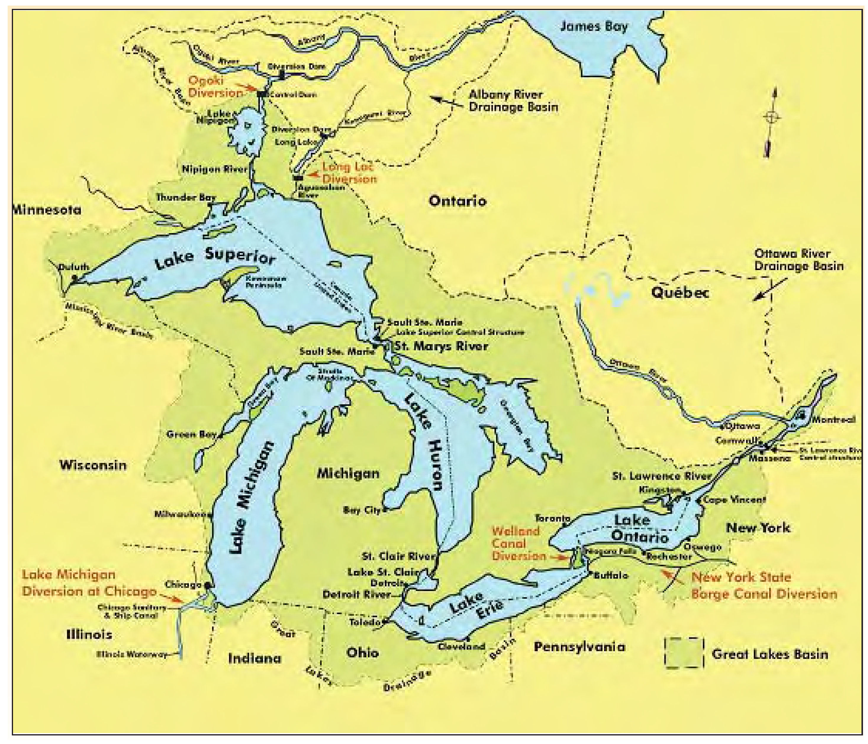
The Great Lakes account for 20% of the Earth’s surface freshwater and for 90% of North America’s surface freshwater [1]. These figures indicate the importance of these lakes as a freshwater reservoir. Furthermore, the Great Lakes have great importance as an ecosystem. With respect to human activities, they are a source of food, they encompass commercial routes for industry, they offer tourist attractions and entire communities and recreational facilities are built around the Great Lakes. A general map of the Great Lakes System can be seen in Figure 1.

Figure 1. Map of the Great Lakes System [2].

Figure 1. Map of the Great Lakes System [2].

Between 1963 and 2006, there has been a lake-to-lake head fall between Lakes Michigan-Huron and Lake Erie of approximately 23 cm. A drop of the water level in the Great Lakes, in addition to translating to a loss of colossal amounts of freshwater, can affect and change the shoreline and the communities that have been built around the Lakes. It may affect the entire ecosystem and can also cause disruptions to human activities, such as creating impediments for the passing of ships. Bathymetric studies indicate that St. Clair River’s conveyance increased during the 1980s; four hydrodynamic models were used during the development of a joint commission report, and all indicated an increase in conveyance [2]. Namely, the models that were used were HEC-RAS (Hydrologic Engineering Centers River Analysis System), RMA-2, HydroSed2D (2D Hydrodynamics and Sediment transport model) and TELEMAC-2D. It is speculated that the increase in conveyance was caused by a deepening of the river related to a major ice jam in 1984 [3]. From the HydroSed2D model, it was estimated that under normal flow conditions, the stresses at the bottom of the St. Clair River would not suffice to induce any bed erosion, considering the bed composition. However, during episodic events, as in ice jam releases, high flow velocities may induce scouring of the bed.

In this work, flow in the St. Clair River is simulated during the presence and the release of an ice jam similar to the one in 1984. A hydrodynamic model is modified in such a way as to simulate the presence of a jam and its subsequent release. A bedload transport model is developed and combined with the hydrodynamic model, and a simulation of the 1984 ice jam release is carried out. The hydrodynamic model is based on the Stanford Unstructured Non-hydrostatic Terrain-following Adaptive Navier–Stokes Simulator (SUNTANS) project [4] and implements the finite volume method to solve the non-hydrostatic Reynolds-averaged Navier–Stokes (RANS) equations on an unstructured z-coordinate grid. The free surface is handled by depth-integration of the continuity equation. Recent ice jam models are based on the St. Venant equations [5,6]. Liu [5] developed a 2D finite element model that treated ice as a separate viscous-plastic continuum. Ice jam release simulations were run with and without the inclusion of ice, and the authors concluded that the presence of ice has a dampening effect on the surge that follows the release of an ice jam, but leads to higher flow velocities after the initial surge. Later, She [6] modified the 1D finite element model by Hicks [7] to account for ice implicitly by adding a resistance term to the momentum equation. Their results were similar to those of Liu [5]. This work marks the first time a fully 3D, non-hydrostatic model was implemented for simulating the presence and release of an ice jam. Complex turbulent structures and non-hydrostatic gradients may affect the stresses on the river bed during the stay and release of an ice jam, and their capture is important in assessing the possible effects on river bed scouring. Furthermore, the hydrodynamic model is computationally efficient at large scales, which is essential in being able to run meaningful simulations in the physical domain involved. The ice jam is modeled as a foreign rigid object in the flow field by setting all fluxes within the ice jam to zero. A drag law is enforced on the underside of the jam to account for flow-induced friction. The ice jam release is simulated by simply removing the zero-flux condition and releasing the initially still body of water in the flow. Several bed scouring models have been developed recently, and all employ a non-hydrostatic RANS solver and all, with the exception of one [8], employ adaptive gridding with continuous meshing [9,10,11,12,13]; the exception being the model by Khosronejad [8] that uses the immersed boundary method.

The scouring model developed in this work is unique in that it employs adaptive gridding without the need for continuous re-meshing. It achieves this by adding or removing cells from the computational domain and the flow field. Unlike the case of the immersed boundary method, the approach followed in this work does not require interpolation for computing boundary flow velocities, since those are readily computed in the finite volume scheme. The hydrodynamic model employs a z-coordinate grid, and the bed is modeled with a step-like approximation. As such, angles of inclination are not readily available for the bed, which are required in order to be able to solve the constitutive relations that give the bedload fluxes. Two different methods for geometric modeling of the river bed are developed and successfully implemented. The methods provide an approach for finding angles of inclination, as well as discretizing the boundary domain in order to solve the Exner equation. Once the bed morphology is modeled, the approach by Roulund [10] is followed to compute the bedload fluxes. In this approach, the equations of motion are solved for a representative bed particle, taking into account not only all the forces involved, but also that the particle may be moving at an angle with the flow. Once the bedload fluxes are computed, the Exner equation is solved numerically, so the approach is contingent upon the geometric modeling methodology for the river bed.

A computational grid is constructed of the St. Clair River, and appropriate bathymetric data are used, as obtained from the Great Lakes Environmental Research Laboratory of the National Oceanic and Atmospheric Administration (NOAA). Boundary conditions are set appropriately, and an ice jam similar to the one in 1984 is modeled. The jam geometric parameters are adjusted so that flow conditions agree with recorded values. Normal flow conditions are also simulated. Finally, flow conditions are simulated with the ice jam in place. Once the steady state is achieved, the stresses on the bed are computed. Then, the ice jam is released, and the bed stresses are computed again.

2. The Hydrodynamic Model

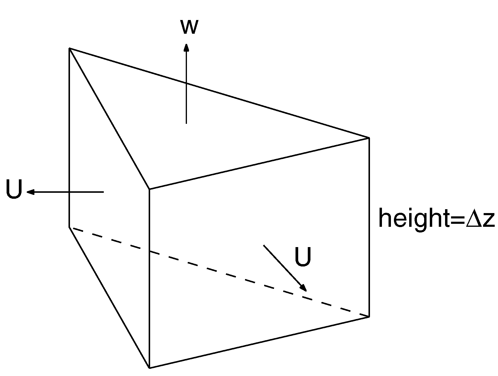
The hydrodynamic model used in this work is a non-hydrostatic, RANS solver that uses the finite volume method on a triangular, z-coordinate staggered grid. It is based on SUNTANS, originally developed by Fringer [4]. A typical cell comprising the grid can be seen in Figure 2.

Figure 2. Description of a 3D prismatic grid cell.

Figure 2. Description of a 3D prismatic grid cell.

The solver computes the horizontal velocity at each vertical face, the vertical velocity at each horizontal face, as well as the free surface height and the non-hydrostatic pressure. The two horizontal momentum equations can be written as follows:

$$\frac{\partial u}{\partial t}+\nabla ·(\overrightarrow{u}u)=-\frac{1}{{\rho }_o}\frac{\partial p}{\partial x}-g\frac{\partial h}{\partial x}+{\nabla }_H·({\nu }_H{\nabla }_{H}u)+\frac{\partial }{\partial z}({\nu }_V\frac{\partial u}{\partial z})$$

(1)

and:

$$\frac{\partial v}{\partial t}+\nabla ·(\overrightarrow{u}v)=-\frac{1}{{\rho }_o}\frac{\partial p}{\partial y}-g\frac{\partial h}{\partial y}+{\nabla }_H·({\nu }_H{\nabla }_{H}v)+\frac{\partial }{\partial z}({\nu }_V\frac{\partial v}{\partial z})$$

(2)

where u and v are the horizontal x and y velocity components, p is the non-hydrostatic pressure, g is the acceleration of gravity and h is the free surface height. ${\nu }_H$ and ${\nu }_V$ are the horizontal and vertical eddy viscosities, following the Boussinesq approximation. Combining the two horizontal momentum equations and taking the dot product with the face normal, $\overrightarrow{n}$, results in:

$$\frac{\partial U}{\partial t}+\overrightarrow{n}·\nabla ·(\overrightarrow{u}\overrightarrow{u})=-\frac{1}{{\rho }_o}\frac{\partial p}{\partial n}-g\frac{\partial h}{\partial n}+{\nabla }_H·({\nu }_H{\nabla }_{H}U)+\frac{\partial }{\partial z}({\nu }_V\frac{\partial U}{\partial z})$$

(3)

where $\frac{\partial }{\partial n}$ is the derivative in the direction of the normal and $\overrightarrow{u}$ is the flow velocity vector. The vertical momentum equation is given by:

$$\frac{\partial w}{\partial t}+\nabla ·(\overrightarrow{u}w)=-\frac{1}{{\rho }_o}\frac{\partial p}{\partial z}+{\nabla }_H·({\nu }_H{\nabla }_{H}w)+\frac{\partial }{\partial z}({\nu }_V\frac{\partial w}{\partial z})$$

(4)

In addition, the incompressibility condition is written as follows:

$$\nabla ·\overrightarrow{u}=0$$

(5)

The free surface is computed by depth-integrating the continuity equation. After enforcement of the kinematic condition at the free surface, an evolution equation for the total depth of flow is obtained, as follows:

$$\frac{\partial h}{\partial t}+\frac{\partial }{\partial x}({\int }_{-d}^{h}u\mathrm{d}z)+\frac{\partial }{\partial y}({\int }_{-d}^{h}v\mathrm{d}z)=0$$

(6)

where d is the depth measured from the undisturbed free surface. The two momentum equations, the depth-integrated continuity equation and the incompressibility constraint form a set of four equations in four unknowns, namely the face-normal velocity, U, the vertical velocity, w, the free surface height, h, and the non-hydrostatic pressure, q. The velocities at the cell centers are found by interpolation.

The boundary condition at the river bed determines the flow resistance using the law of the wall and can be written as follows:

$${\nu }_V\frac{\partial U}{\partial z}{|}_{z=h}=C_{d,B}\left|U\right|U$$

(7)

where $C_{d,B}$ is the drag coefficient for the bed.

In the numerical scheme for the momentum equations, the convection and horizontal diffusion terms are discretized explicitly. Vertical diffusion terms are discretized semi-implicitly with the theta method. The semi-implicit treatment of vertical diffusion terms, as opposed to the explicit treatment of other diffusion and convection terms, allows for the use of smaller discretization scales in the vertical direction, while keeping a relatively large time step. This makes SUNTANS suitable for simulations in estuaries, rivers and oceans, where horizontal scales are much bigger than vertical ones.

The non-hydrostatic solver uses a predictor-corrector method. The velocity field is predicted based on the non-hydrostatic pressure of the previous time step. The momentum equations are solved jointly with the depth-integrated continuity equation, where the predicted horizontal velocity is used, to give the predicted velocity field, as well as the free surface height at the next time step. The predicted velocity field is then inserted into the local continuity equation, and a Poisson equation is solved for the non-hydrostatic pressure correction term at the next time step. Once the correction term is computed, the velocity and pressure fields are updated to those of the next time step.

2.1. The Turbulence Model

Closure to the RANS equations is achieved with the Mellor and Yamada 2.5 model. The key characteristic of the model is that it applies to situations where the horizontal scales are much bigger than the vertical scales, and as such, it is assumed that turbulence is resolved only in the latter. Only the vertical eddy viscosity is solved for, while the horizontal eddy viscosity is set to a constant in order to preserve stability. The vertical eddy viscosity is given by:

$${\nu }_V=-lq{S}_M$$

(8)

where l is a length scale, q is the turbulent kinetic energy and $S_M$ is an algebraic function of the vertical horizontal velocity gradients. The Mellor and Yamada model is a two-equation model. The equation for the turbulent kinetic energy is given by:

$$\frac{D(q^2/2)}{Dt}-\frac{\partial }{\partial z}(lq{S}_q\frac{\partial }{\partial }(\frac{q^2}{2})=P_s-ϵ$$

(9)

where $S_q$ is a constant and ϵ is the turbulent kinetic energy dissipation rate given by:

$$ϵ=\frac{q^3}{B_{1}l}$$

(10)

The dissipation rate is inversely proportional to the length scale, since the latter represents an average distance that a turbulent eddy travels before it is dissipated. The equation for the length scale is given by:

$$\frac{D}{Dt}(q^{2}l)-\frac{\partial }{\partial z}[ql{S}_l\frac{\partial }{\partial z}(q^{2}l)]=l{E}_1{P}_s-\frac{q^3}{B_1}[1+E_2{(\frac{l}{\kappa L})}^2]$$

(11)

where $S_l$, $E_1$ and $E_2$ are constants, κ is the von Karman constant and L is the distance from the wall.

3. The Bed Scouring Model

The boundary condition that the hydrodynamic model uses for the bed is given by Equation (7) and is based on the law of the wall. It can be shown that the drag coefficient, $C_{d,B}$, is given by:

$$C_{d,B}={(\frac{1}{\kappa }ln\frac{z}{z_o})}^{-2}$$

(12)

where z is the distance from the bed at which the velocity is measured and $z_o$ is the theoretical distance from the bed at which the velocity becomes zero. For rough boundaries, $z_o$ is given by:

$$z_o=\frac{k_s}{30}$$

(13)

where $k_s$ is the equivalent roughness height. For typical river beds, $k_s$ can be taken as [14]:

$$k_s\approx 3.5d_{85}$$

(14)

where $d_{85}$ is the the 85th percentile grain diameter. Generally, $d_{85}$ can be taken to be 1.5 times the median grain diameter, $d_{50}$, of the bed [15]. If the sediment size and type are known, the shear velocity can be computed by measuring the flow velocity some distance z above the bed and taking:

$$u_{*}=\sqrt{{(\frac{1}{\kappa }ln\frac{z}{\frac{3.5*1.5*d_{50}}{30}})}^{-2}}\left|U\right|$$

(15)

The dimensionless Shields stress, θ, can then be calculated using the formula:

$$\theta =\frac{u_{*}^2}{(s-1)g{d}_{50}}$$

(16)

where s is the specific gravity of the sediment. In the model, both the median sediment grain size, $d_{50}$, and the specific gravity can vary along the bed, with the resolution of the field distribution being limited only by the resolution of the horizontal mesh.

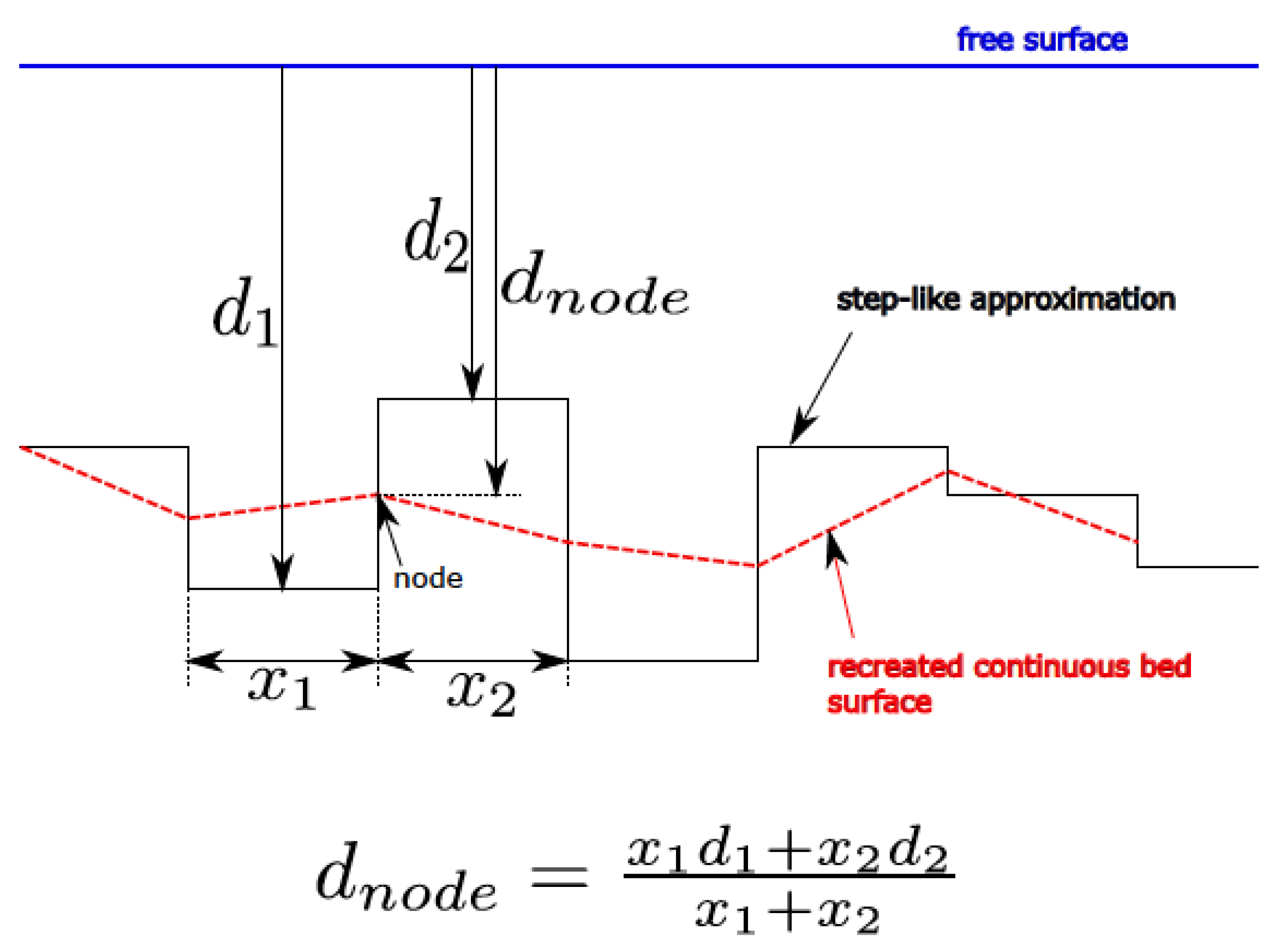
The constitutive relations that couple the flow field with sediment movement at some point along the bed require that the local angle of inclination of the bed at that location be known. SUNTANS implements a step-like approximation of the bed, and as such, local angles of inclination are not readily available. Two different approaches were developed in order to estimate the angle of inclination. In both methods, the bathymetry is approximated by projecting the horizontal triangular mesh on the plane of the bed. In the first method, each vertex of a triangle is assigned a depth equal to the weighted average of the depths of the Voronoi points of triangles that share that vertex. Figure 3 shows a schematic of the two-dimensional equivalent case.

Figure 3. Reconstructing the bed geometry: the 2D case. The red dotted line is the reconstructed continuous surface.

Figure 3. Reconstructing the bed geometry: the 2D case. The red dotted line is the reconstructed continuous surface.

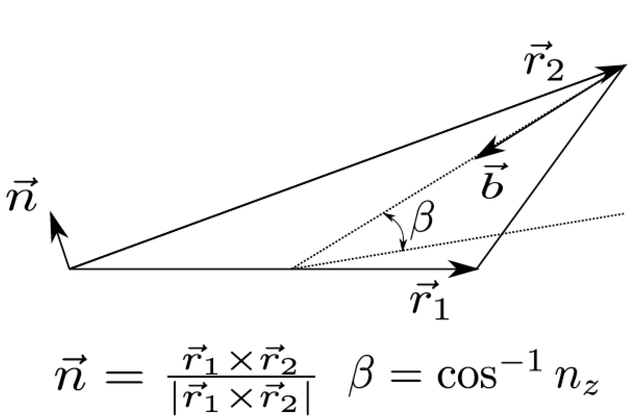
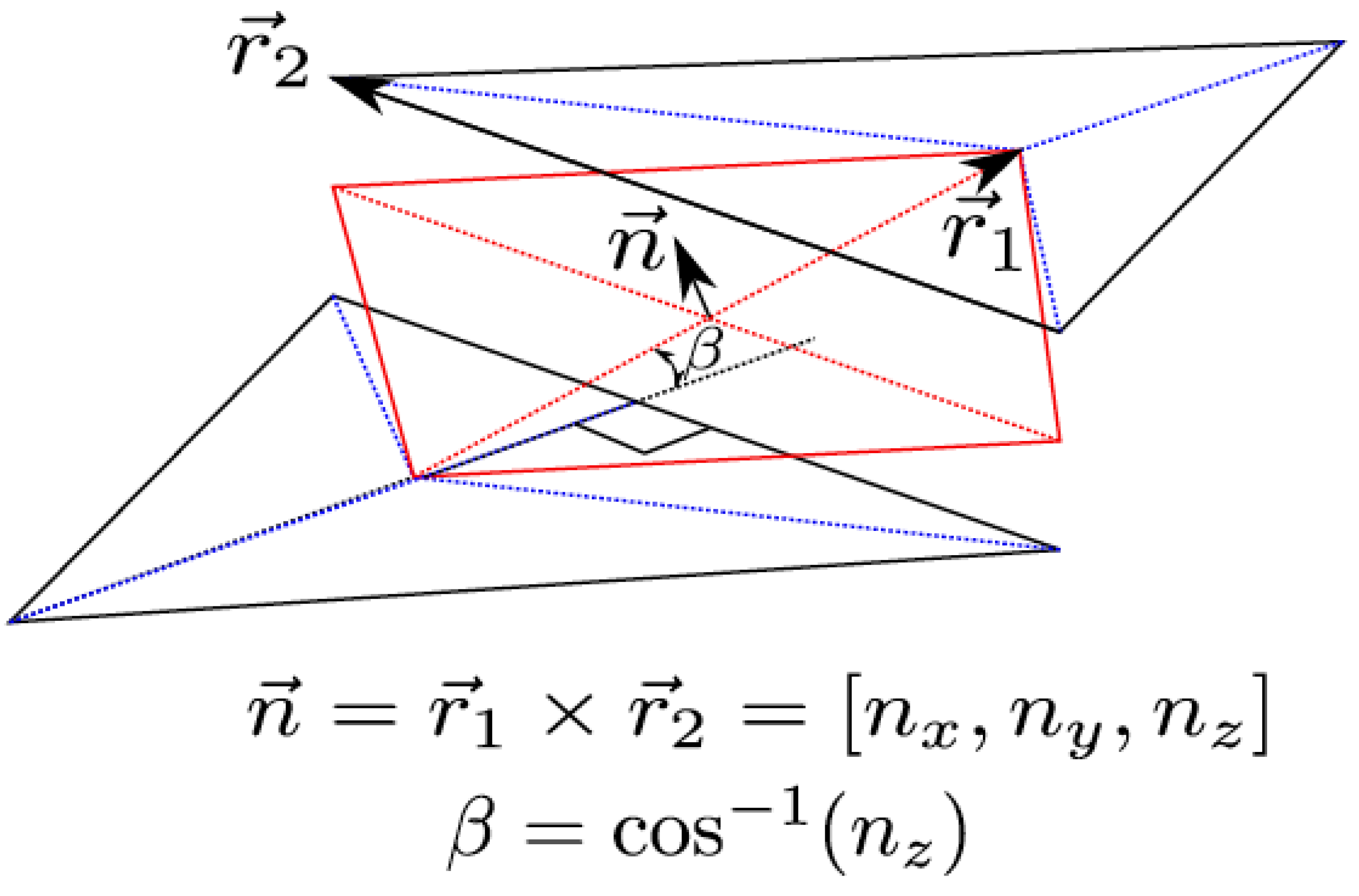
As shown in Figure 4, the angle of inclination is just the inverse cosine of the z-component ($n_z$) of the normal vector, $\overrightarrow{n}$. The direction of maximum slope, given by the vector, $\overrightarrow{b}$, along which the weight component acts, is given by:

$$\overrightarrow{b}=\frac{({\widehat{e}}_z\times \overrightarrow{n})\times \overrightarrow{n}}{|({\widehat{e}}_z\times \overrightarrow{n})\times \overrightarrow{n}|}$$

(17)

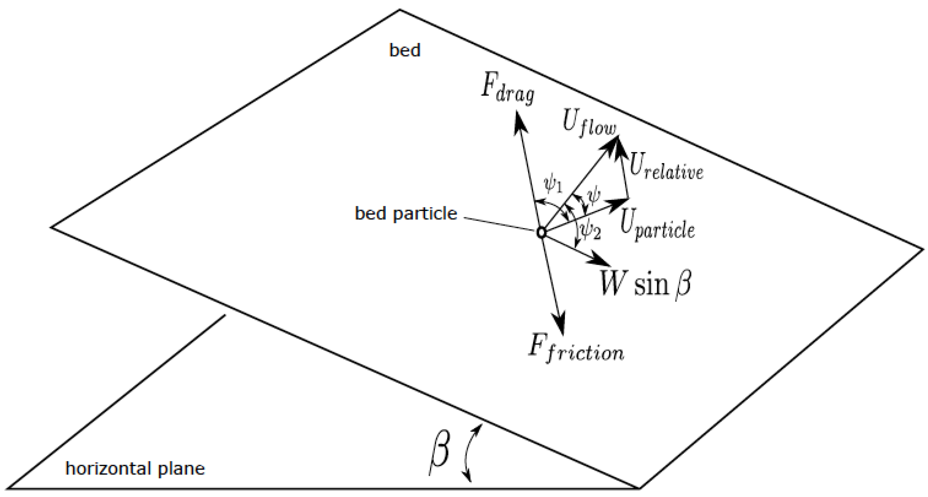
where ${\widehat{e}}_z$ is the unit vector in the z-direction. Once these important geometric parameters are known, i.e., the angle of inclination and the direction of maximum slope, the flow field can be coupled with sediment transport. The key coupling factor is the shear velocity, which is essentially a measure of the stress on the bed. The application of the constitutive relations follow the approach by Roulund [10], where a force balance is applied to a representative sediment particle. The schematic shown in Figure 5 shows the forces involved, as well as their geometric relationships.

Figure 4. Finding the bed inclination.

Figure 4. Finding the bed inclination.

Figure 5. Forces on a bed particle and their geometric relationships.

Figure 5. Forces on a bed particle and their geometric relationships.

A set of dynamic and kinematic non-linear algebraic relations are produced and solved in our model by the Newton–Raphson method. The solution to the system of equations provides the velocity of the representative particle, which is then extrapolated to compute the bed load fluxes along the bed. Once the fluxes are known, a bed evolution equation is solved, also known as the Exner equation, given below:

$$\frac{\partial \eta }{\partial t}=-\frac{1}{1-n}\nabla ·{\overrightarrow{q}}_b$$

(18)

where η is the bed elevation, n is the sediment porosity and ${\overrightarrow{q}}_b$ are the 2D fluxes. Integrating over an element and applying the divergence theorem gives:

$$A\frac{\partial \eta }{\partial t}=-\frac{1}{1-n}{\int }_{\partial A}{\overrightarrow{q}}_b·\overrightarrow{n}$$

(19)

where $\overrightarrow{n}$ is the outward normal and A is the projected area of an element. Discretization of the last equation yields:

$$\frac{\Delta {\eta }_i}{\Delta t}=-\frac{1}{1-n}\frac{1}{A_i}\sum _{j=1}^3{\overrightarrow{q}}_j·{\overrightarrow{n}}_j{l}_j$$

(20)

where the index, i, refers to the cell number and the index, j, refers to the number of the side of the cell. $l_j$ is the length of side j. In this method of geometric modeling of the bed, the fluxes are initially computed at the cell centers. The fluxes at the sides are computed by simple interpolation.

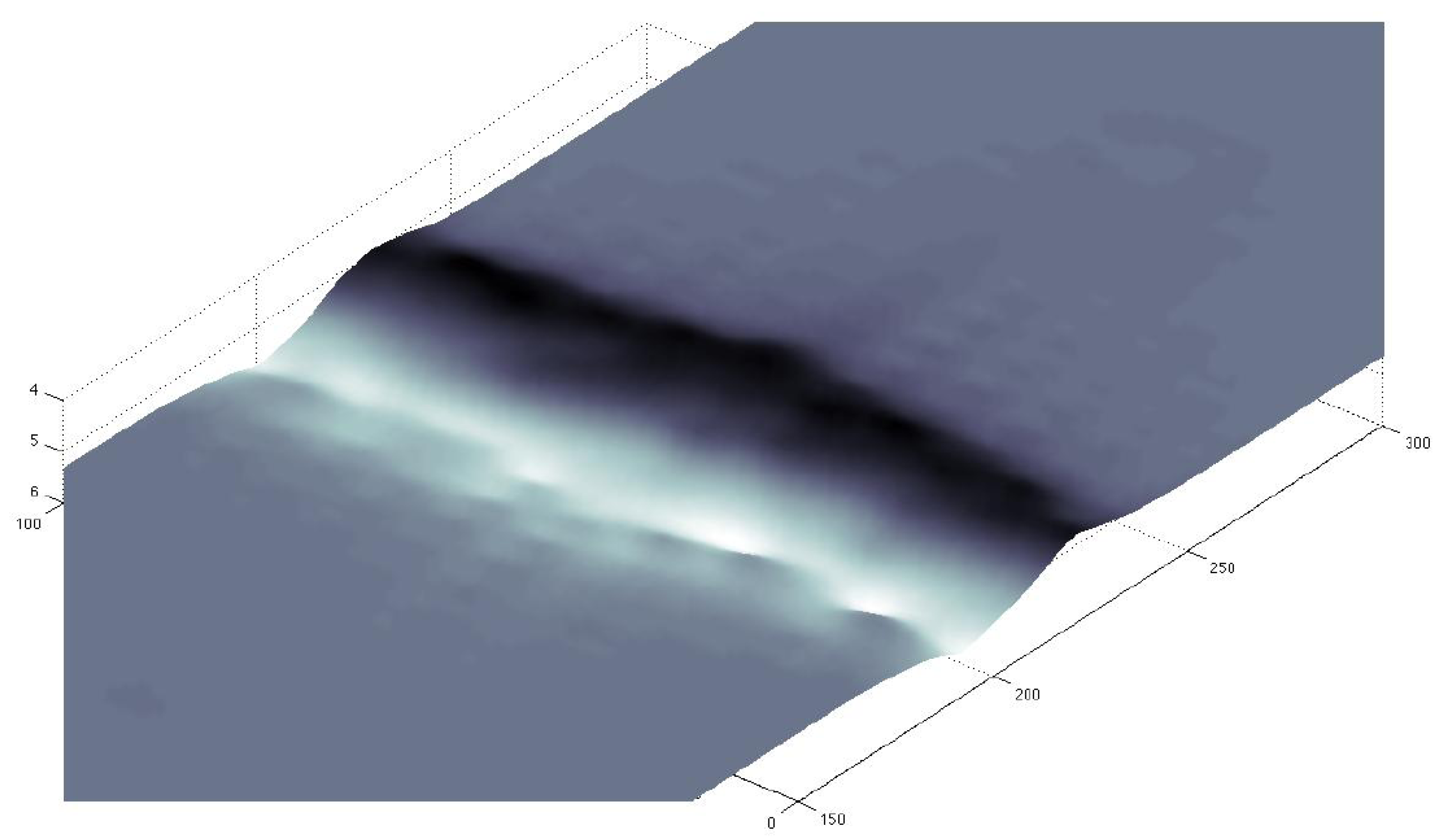
The aforementioned model was used to simulate the scouring downstream of a sluice gate. The specifics of the computational setup are given by [16]. The computed bed surface is shown in Figure 6. While the results are qualitatively correct, a noticeable irregularity is present. The errors are a direct result of the averaging process proposed above for the computation of the local angels of inclination. Although artificial diffusion has been added to the Exner equation, the erratic bed scouring persists.

Figure 6. Scouring under a sluice gate.

Figure 6. Scouring under a sluice gate.

To avoid the irregularities that result from the geometric modeling technique, an alternative method was developed and used in the simulations. Figure 7 explains schematically the proposed method. It involves the division of each element in three parts and the assignment of a different angle of inclination to each part. The angle is shared by the corresponding part of the adjacent cell, depending on the depth difference between the two cells.

Figure 7. The geometric scheme followed in order to find the bed inclination.

Figure 7. The geometric scheme followed in order to find the bed inclination.

The constitutive relations are then solved separately for each part of the cell, but always using the shear velocity derived at the center of the cell. Therefore, each part of the cell has a different flux assigned to it. Fluxes at the edges are computed by simple interpolation, and the Exner equation is solved accordingly, following the procedure presented above.

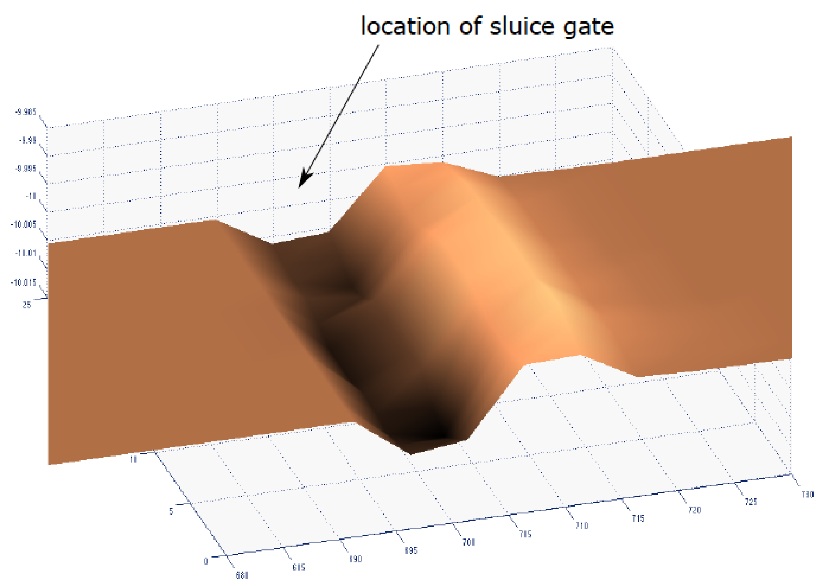
Figure 8 depicts scouring under a sluice gate, under the same flow conditions, i.e., those used to produce the results in Figure 6. The superiority of the alternative method is obvious, as no irregularities appear in the solution of the Exner equation, and no artificial diffusion is needed.

Figure 8. Scouring under a sluice gate (not shown) with the latter modeling scheme. No irregularities are present.

Figure 8. Scouring under a sluice gate (not shown) with the latter modeling scheme. No irregularities are present.

While the bed morphology used for bed scouring is not exactly interpreted by the hydrodynamic model, since it implements step-like approximation, the z-coordinate meshing offers an advantage over other existing models. An algorithm was developed and implemented, whereby the grid adapts to the changing bed by shrinking or elongating the cells nearest to the bottom when the change in bed elevation is small. However, when the change in bed elevation exceeds a certain threshold, cells are added or removed from the computational grid. This allows the grid to adapt to any change in bed morphology, however great that may be, by not having to re-mesh the entire domain and by avoiding any grid distortions if the change is significant. At the same time, velocities at the center of cells are readily available from the hydrodynamic model, which allows for easy computing of the shear velocity without the need for any interpolation, as would be the case in an immersed boundary method. Overall, with the hydrodynamic model being well-suited for large-scale flows and the scouring model being able to accommodate for changing bathymetry without significant computational cost, the combined model is well suited for scouring simulations in rivers.

4. Ice Jam Release Scenario

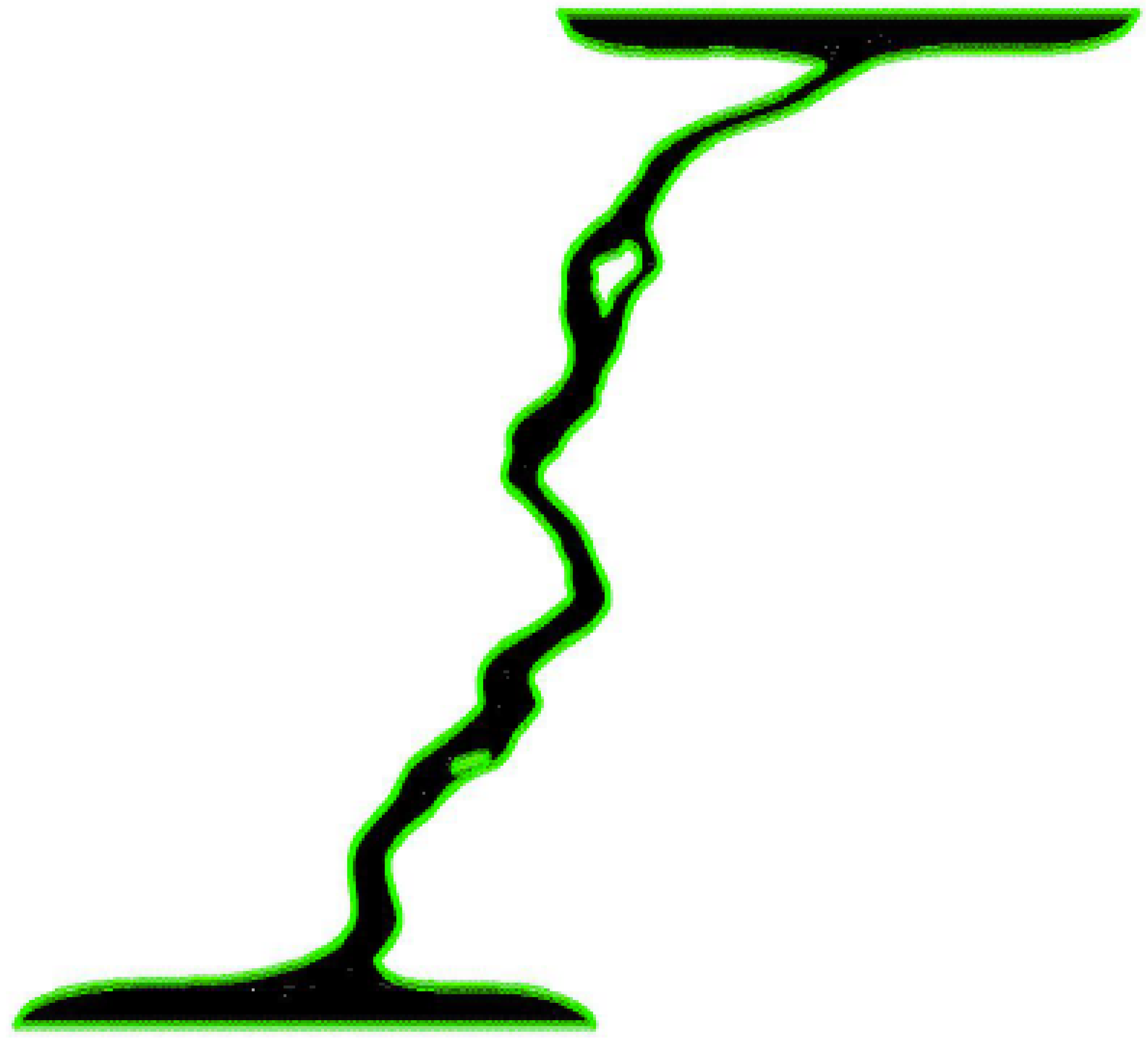
The 1984 ice jam in the St. Clair River was chosen as a case scenario. Simulations were first run under conditions where an ice jam was not present. The boundary conditions used were fixed stage elevations at the entrance and exit of the river, no slip at the banks and the law of the wall for the bed. The effect of wind-induced stresses was neglected. The entrance and exit of the river were constructed to be very wide in our grid, as can be seen in Figure 9, and the flow velocities at the cells forming the boundaries of the entrance and exit were set to zero. Weak boundary conditions were enforced at the entrance and exit to allow for mass flow, as dictated by the difference in stage elevations.

The bathymetry was determined from data obtained from NOAA, along with the sediment size distribution in the river [17]. The bathymetric data had a resolution of approximately 60 m, which was comparable to the resolution of the grid(s) used. Varying the size of the sediment along the river bed allowed for variation in the bed drag coefficient. The stage elevation difference between the entrance of the St. Clair River and its estuary remains almost constant over the seasons and equal to approximately 1.4 m. The seasonal variation in flow rates is due to the water level in the river. The bathymetric data obtained from NOAA were adjusted by adding approximately 15 $cm$ uniformly to the depth of the river in order to achieve a flow rate of approximately 4800 $m^3/sec$, which is a reasonable estimate for the month of April. The flow rates obtained from NOAA were based on year-averaged values. Furthermore, it was found that varying the depth of the river in our model within the limits of measured average seasonal variations caused flow rates to vary within the range of reported seasonal values with a 95% approximate accuracy; this agreement added credibility to the hydrodynamic model, as well as the bed roughness values used, dependent on the sediment size distribution. Under average flow conditions, it was found that there are three regions of elevated stresses along the river, as can be seen in Figure 10.

Figure 9. Grid used for our simulations.

Figure 9. Grid used for our simulations.

Figure 10. Stress distribution (Shields stress values) in the St. Clair River under average flow conditions. There are three regions of elevated stresses on the bed (yellow and red colors).

Figure 10. Stress distribution (Shields stress values) in the St. Clair River under average flow conditions. There are three regions of elevated stresses on the bed (yellow and red colors).

The ice jam was simulated by setting all fluxes to zero in the flow field region occupied by the jam. The size of the zero-flux region was adjusted so that flow conditions agree with the recorded values during the 1984 ice jam. In the final days of the jam, the water flow through the river was reduced by approximately 65% and the water level in Lake St. Clair dropped by approximately 0.6 m. In our model, the stage elevation at the exit of the river was reduced by 0.6 m and the size and the thickness of the jam was adjusted so that the flow rate become approximately 1700 $m^3/s$. The adjusted ice jam configuration and the resulting flow rate served as an initial condition for the ice jam release simulation. The ice jam in our model, in its final form, had a head thickness of 2 m and gradually thickened to reach a thickness of 4 m at its toe, which is a shape similar to that of an actual ice jam. Detailed information on the shape of the 1984 ice jam is lacking. The length of the ice jam was in accordance to field observations of the 1984 ice jam [3]. In its final days, the ice jam covered about a third of the river, its upstream end starting a little below St. Clair and its downstream end reaching Algonac. A drag law was imposed on the under side of the ice jam, to account for friction between the flow and the ice. A friction coefficient in accordance with published data was chosen [18]. It was found that the stresses on the bed under the still ice jam were lower than those when an ice jam was not present. This is in disagreement with the assertion that scouring would happen under the toe of the fully developed ice jam.

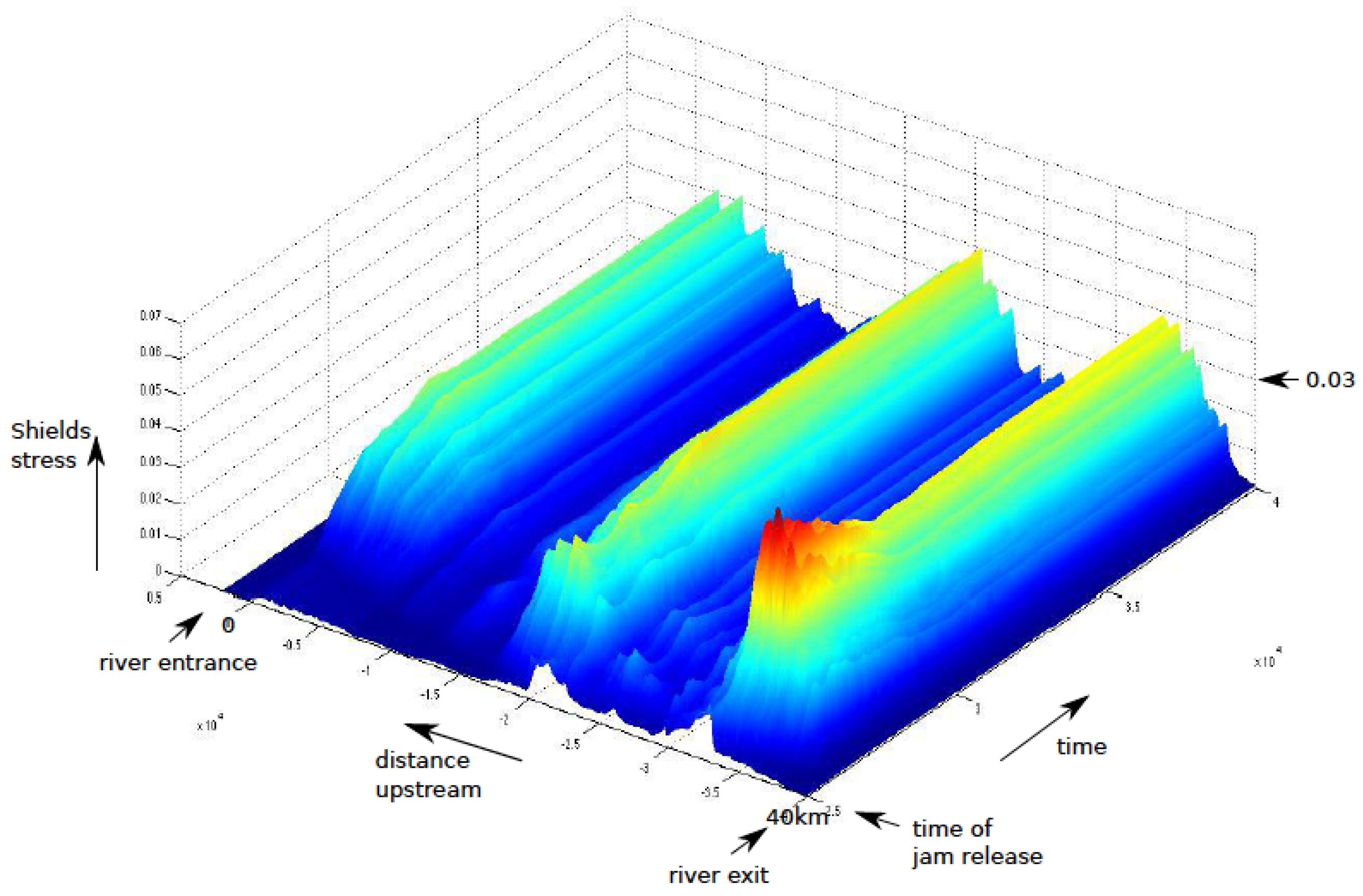
The ice jam was released by removing the zero-flux condition. Figure 11 shows the stress evolution on the river bed following the release.

Figure 11. Evolution of stresses on the river bed following the release of a jam.

Figure 11. Evolution of stresses on the river bed following the release of a jam.

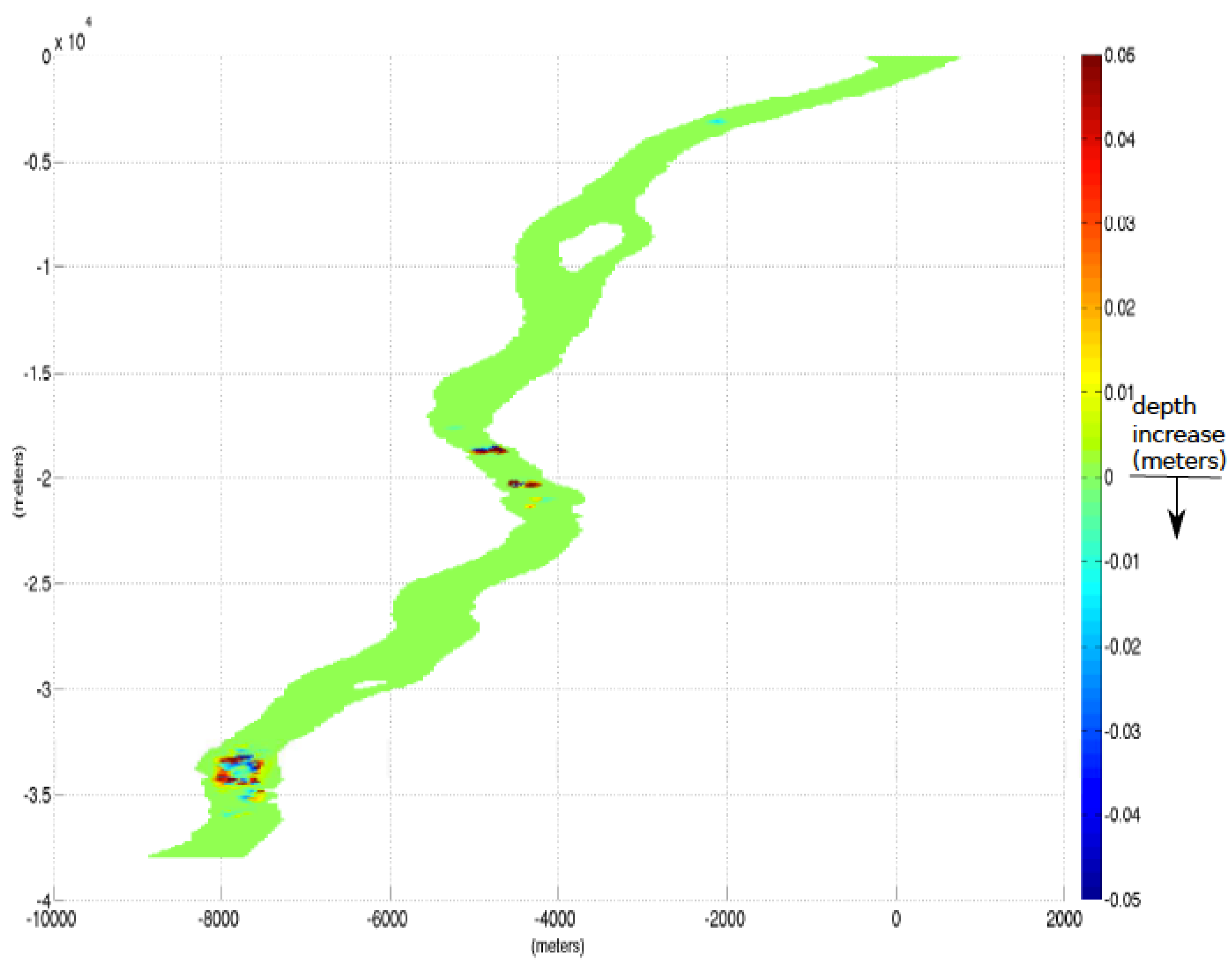
It can be seen from the figure that the stresses in three regions are particularly high. These are the regions that experience high stresses when an ice jam is absent, according to the model. A critical Shields stress value of 0.03 was chosen. The critical Shields stress value varies depending on the kind of sediment that comprises the surface layer of the bed. For a bed with a uniform grain size, the nominal value of 0.047 is given [19,20]. However, based on experimental studies and field observations of bedload transport in rivers, for beds with mixed grain composition, a value of 0.03 is more accurate [21,22,23]. The critical Shields stress was adjusted for the local angle of inclination at each computational cell. It was found that critical stress values were exceeded in the three regions of elevated stresses on the river bed, with ensuing scouring. Most scouring occurred near the exit of the river. Figure 12 depicts the depth change caused by scouring during the first 1.4 h following the release.

Figure 12. The change in depth along the river caused by scouring.

Figure 12. The change in depth along the river caused by scouring.

The net amount of sediment displaced during that period was approximately 10,000 cubic meters. Most of the scouring occurred near the estuary in Lake St. Clair, at the exit of the river. It is concluded that in the case of an ice jam similar to the one in 1984, scouring is highly probable following the release of the ice jam. While our results do not constitute proof that scouring of such an extent will happen, they provide a strong indication. The results are based on a particular hydrodynamic model and a particular turbulence model; other hydrodynamic and turbulence models should be implemented before drawing final conclusions. Three different grids were used as part of grid refinement studies: One with approximately 600,000 cells, one with approximately one million cells and the most refined, which had approximately two million cells. The three grids had a horizontal spacing of approximately 55, 45 and 35 m, respectively, while the vertical grid spacing ranged from 1 m to 75 $cm$. The results in terms of scouring were similar for all three grids.

5. Conclusions

A bed scouring model was developed and incorporated in a hydrodynamic model that implements a z-coordinate grid with step-like approximation of the river bed. An algorithm that expands or contracts the grid to follow changes in bed morphology without the need for re-meshing the entire grid was also developed. Ice jams were modeled by creating a rigid body of water in the flow field by ignoring the fluxes in the cells that comprise the region of the ice jam. The release was simulated by removing the zero-flux condition and releasing the initially stationary body of water into the flow field. The 1984 ice jam in the St. Clair River was simulated by adopting flow and boundary conditions that replicate the conditions during the jam. It was found that in the scenario of a jam like the one in 1984, scouring occurs that amounts to significant net amounts of displaced sediment, especially near the river exit. The effect of such a change in bed morphology on the river’s conveyance needs to be ascertained, and the sensitivity of the system to changes in depth in the locations affected by the ice jam release remains a subject of future research. The present model provides a framework for the prediction of extreme events in the Huron-Erie Corridor and for designing mitigation measures.

References

- Great Lakes Information Network. Available online: http://www.great-lakes.net (accessed on 30 September 2013).
- International Joint Commission. Impacts on Upper Great Lakes Water Levels: St. Clair River; International Upper Great Lakes Study: Ottawa, ON, Canada, 2009. [Google Scholar]
- Derecki, J.A.; Quinn, F.H. Record St. Clair River ice jam of 1984. J. Hydraul. Eng. 1986, 112, 1182–1194. [Google Scholar]
- Fringer, O.B.; Gerritsen, M.; Street, R.L. An unstructured-grid, finite-volume, nonhydrostatic, parallel coastal ocean simulator. J. Ocean. Model. 2006, 14, 139–173. [Google Scholar] [CrossRef]
- Liu, L.W.; Shen, H.T. Dynamics of ice jam release surges. In Proceedings of the 17th International Symposium on Ice, St. Petersburg, Russia, 21–25 June 2004.
- She, Y.; Hicks, F. Incorporating ice effects in ice jam release surge models. In Proceedings of the 13th Workshop on the Hydraulics of Ice Covered Rivers, Hanover, ON, Canada, 15–16 September 2005.
- Hicks, F.; Steffler, P.M. Characteristic dissipative Galerkin scheme for open channel flow. J. Hydraul. Eng. 1992, 118, 337–352. [Google Scholar] [CrossRef]
- Khosronejad, A.; Seokkoo, K.; Borazjani, I.; Sotiropoulos, F. Curvilinear immersed boundary method for simulating coupled flow and bed morphodynamic interactions due to sediment transport phenomena. Adv. Water Resour. 2011, 34, 829–843. [Google Scholar] [CrossRef]
- Nagata, N.; Hosoda, T.; Nakato, T.; Muramoto, Y. Three-dimensional numerical model for flow and bed deformation around river hydraulic structures. J. Hydraul. Eng. 2005, 131, 1074–1087. [Google Scholar] [CrossRef]
- Roulund, A.; Sumer, B.M.; Fredsoe, J.; Michelsen, J. Numerical and experimental investigation of flow and scour around a circular pile. J. Fluid Mech. 2005, 534, 351–401. [Google Scholar] [CrossRef]
- Khosronejad, A.; Rennie, C.D.; Salehi, S.A.A.; Townsend, R.D. 3D numerical modeling of flow and sediment transport in laboratory channel bends. J. Hydraul. Eng. 2007, 133, 1123–1134. [Google Scholar] [CrossRef]
- Liu, X.; Garcia, H.M. Three-dimensional numerical model with free water surface and mesh deformation for local sediment scour. J. Waterw. Port Coast. Ocean Eng. 2008, 134, 203–217. [Google Scholar] [CrossRef]
- Apsley, D.D.; Stansby, P. Bed-load sediment transport on large slopes: Model formulation and implementation within a RANS solver. J. Hydraul. Eng. 2008, 134, 1440–1451. [Google Scholar] [CrossRef]
- Haws, B.B. Ability of ADV Measurements to Detect Turbulence Differences Between Angular and Rounded Gravel Beds of Intermediate-Roughness Scale. Master’s Thesis, Brigham Young University, Provo, UT, USA, 2008. [Google Scholar]
- Raudviki, A.J. Loose Boundary Hydraulics; Balkema: Rotterdam, The Netherlands, 1998. [Google Scholar]
- Manolidis, M. Modeling the Release of River Ice Jams and their Impact on River Bed Scouring. Ph.D. Thesis, University of Michigan-Ann Arbor, Ann Arbor, MI, USA, 2013. [Google Scholar]
- Krishnappan, B.G. Sediment transport regime of St. Clair River. In Sediment Studies in St. Clair River; International Upper Great Lakes Study Board of the International Joint Commission: Ottawa, ON, Canada, 2009. [Google Scholar]
- Attar, S.; Li, S.S. Momentum, Energy and Drag Coefficients for Ice-Covered Rivers. River Res. Appl. 2012. [Google Scholar] [CrossRef]
- Meyer-Peter, E.; Muller, R. Formulation for Bed Load Transport. In Proceedings of the 2nd Congress, International Association of Hydraulic Research, Stockholm, Sweden, 7–9 June 1948.
- Einstein, H.A. The Bed Load Function for Sediment Transportation in Open Channel Flows; Technical Bulletin of U.S. Department of Agriculture: Washington, DC, USA, 1950. [Google Scholar]
- Parker, G. Surface-Based Bedload Transport Relation for Gravel Rivers. J. Hydraul. Res. 1990, 28, 417–436. [Google Scholar] [CrossRef]
- Duan, J.G.; Scott, S. Selective Bed Load Transport in Las Vegas Wash, a Gravel-Bed Stream. J. Hydrol. 2007, 342, 320–330. [Google Scholar] [CrossRef]
- Wilcock, P.R.; Kenworthy, S.T.; Crowe, J.C. Experimental Study of the Transport of Mixed Sand and Gravel. Water Resour. Res. 2001, 37, 3349–3358. [Google Scholar] [CrossRef]
© 2014 by the authors; licensee MDPI, Basel, Switzerland. This article is an open access article distributed under the terms and conditions of the Creative Commons Attribution license (http://creativecommons.org/licenses/by/3.0/).
Share and Cite
MDPI and ACS Style
Manolidis, M.; Katopodes, N. Bed Scouring During the Release of an Ice Jam. J. Mar. Sci. Eng. 2014, 2, 370-385. https://doi.org/10.3390/jmse2020370
AMA Style
Manolidis M, Katopodes N. Bed Scouring During the Release of an Ice Jam. Journal of Marine Science and Engineering. 2014; 2(2):370-385. https://doi.org/10.3390/jmse2020370
Chicago/Turabian StyleManolidis, Michail, and Nikolaos Katopodes. 2014. "Bed Scouring During the Release of an Ice Jam" Journal of Marine Science and Engineering 2, no. 2: 370-385. https://doi.org/10.3390/jmse2020370