
Modeling Water Clarity and Light Quality in Oceans

Atlantic Ecology Division, National Health and Environmental Effects Research Laboratory, Office of Research and Development, United States Environmental Protection Agency, 27 Tarzwell Drive, Narragansett, RI 02882, USA
J. Mar. Sci. Eng. 2016, 4(4), 80; https://doi.org/10.3390/jmse4040080
Submission received: 20 July 2016
/
Revised: 25 October 2016
/
Accepted: 18 November 2016
/
Published: 24 November 2016
(This article belongs to the Special Issue Selected Papers from the 14th Estuarine and Coastal Modeling Conference)
Abstract
:Phytoplankton is a primary producer of organic compounds, and it forms the base of the food chain in ocean waters. The concentration of phytoplankton in the water column controls water clarity and the amount and quality of light that penetrates through it. The availability of adequate light intensity is a major factor in the health of algae and phytoplankton. There is a strong negative coupling between light intensity and phytoplankton concentration (e.g., through self-shading by the cells), which reduces available light and in return affects the growth rate of the cells. Proper modeling of this coupling is essential to understand primary productivity in the oceans. This paper provides the methodology to model light intensity in the water column, which can be included in relevant water quality models. The methodology implements relationships from bio-optical models, which use phytoplankton chlorophyll a (chl-a) concentration as a surrogate for light attenuation, including absorption and scattering by other attenuators. The presented mathematical methodology estimates the reduction in light intensity due to absorption by pure seawater, chl-a pigment, non-algae particles (NAPs) and colored dissolved organic matter (CDOM), as well as backscattering by pure seawater, phytoplankton particles and NAPs. The methods presented facilitate the prediction of the effects of various environmental and management scenarios (e.g., global warming, altered precipitation patterns, greenhouse gases) on the wellbeing of phytoplankton communities in the oceans as temperature-driven chl-a changes take place.
1. Introduction
The major factors affecting phytoplankton metabolism are nutrient availability, light and water temperature [1]. The maximum depth at which light intensity is adequate to maintain the plant is referred to as the depth of the photic (or euphotic) zone, which is referred to here as the “photic depth” [2]. Light intensity at this depth reaches 1% of its surface daylight value, which is enough for photosynthesis to sustain phytoplankton growth and reproduction. This depth can change as the incident solar irradiance changes with time during the day and throughout the year. The photic depth can also change in space as the concentrations of the various attenuators above it change.
The importance of light to phytoplankton has driven many researchers to develop quantitative methods to calculate light intensity in the water column. The complexity of this task arises from the variability not only in the spectral light intensity, but also in the water column due to turbidity. Bio-optical models are used to develop mathematical methods to calculate irradiance through the water column [3]. Optical models have to be calibrated based on field measurements of both water turbidity from phytoplankton, colored dissolved organic matter (CDOM) (also called yellow substances or Gelbstoff) and non-algae (non-pigmented) particles (NAPs), as well as associated spectral irradiance [4,5,6,7,8,9]. Abdelrhman [10] applied these methods to estuarine systems where both phytoplankton and total suspended solids (TSS) contribute to turbidity. In oceans, the major contributor to turbidity is phytoplankton [11,12]. The theoretical basis presented in [12] was further simplified here to accommodate numerical modelers’ needs. Prieur and Sathyndranath [13] presented the optical classification of coastal and oceanic waters based on the specific spectral absorption curves of phytoplankton pigments, organic matter and other attenuators of light in the water column. A wide range of absorption and backscattering spectra for oceans was presented by the International Ocean Color Coordination Group (IOCCG) [3]. The IOCCG generated a wide range of synthetic data for use in testing remote sensing algorithms. This range was based on mathematical relationships that used measured phytoplankton concentration in ocean waters (Case 1 waters [14]) as a reference for absorption and backscattering by all other attenuators in the water column including NAPs and CDOM. These relationships are used here to calculate irradiance throughout the water column in the oceans.
The focus of this work is determining the available irradiance profile in the water column through the photic depth. The concentration of suspended solids and phytoplankton in the water column controls the amount of light that travels through it. The main objective of this work is to present a mathematical model, which can be included in numerical models, to resolve the coupling between irradiance and phytoplankton in the oceans. This objective is met by focusing on using available information from bio-optical methods, rather than developing them. Inherent optical properties of water (i.e., chl-a concentrations) [3] are used to meet the modeling objective.
2. Methods
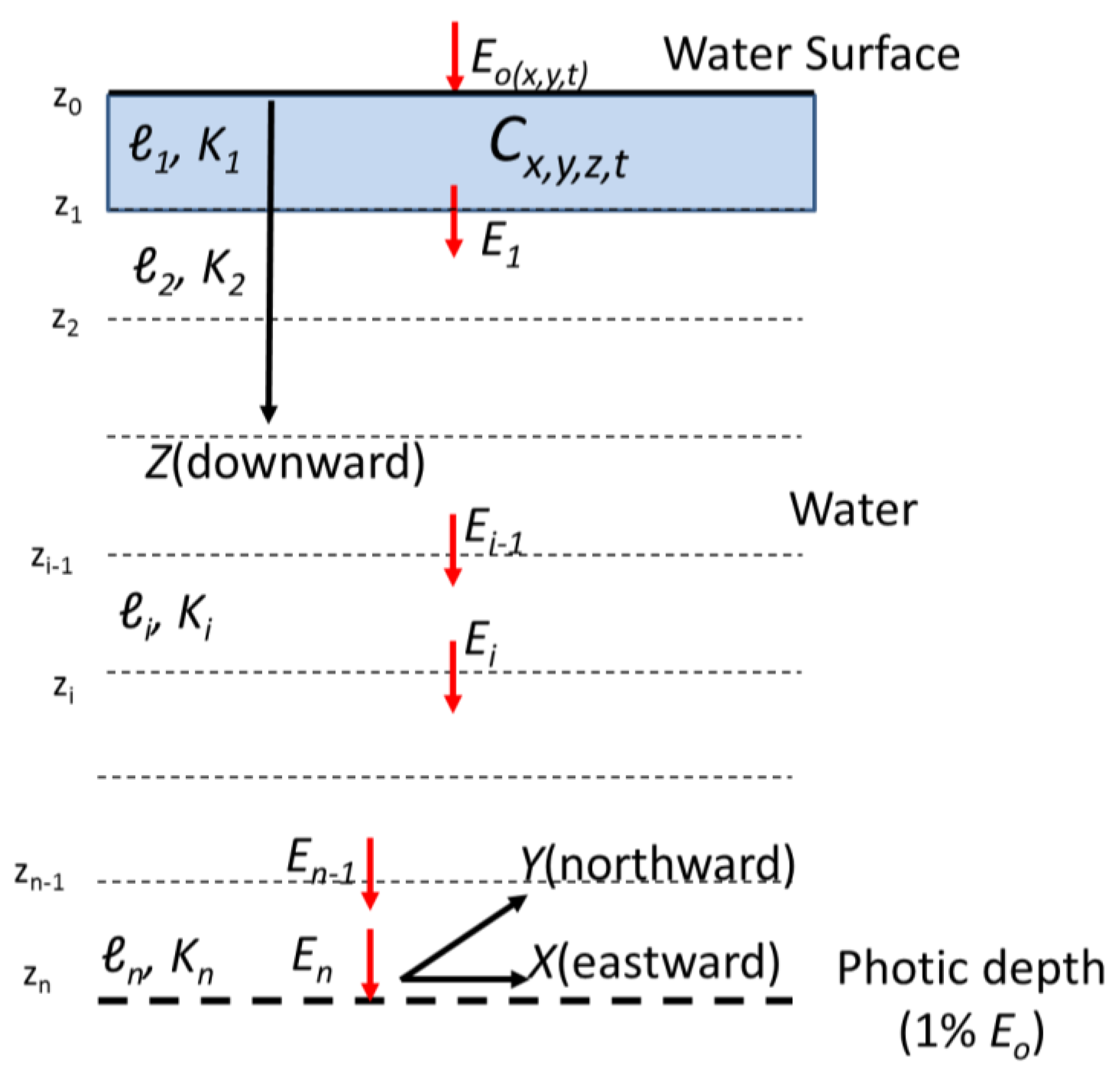
The total concentration of chl-a is obtained from available field measurements and used to develop the mathematical methodology to estimate the irradiance throughout the water column at any location throughout the whole year. Figure 1 presents a definition sketch of the vertical structure for the mathematical model for irradiance, and Table 1 presents the definitions of all abbreviations and symbols. Attenuation of the incident irradiance through the water column is a function of absorption and scattering by the pure seawater and the dissolved and particulate materials therein.
There are seven major contributors to the loss of light intensity through the water column: (1) absorption by pure seawater; (2) absorption by phytoplankton (algae) pigment; (3) absorption by NAPs; (4) absorption by CDOM; (5) backscattering by phytoplankton particles; (6) backscattering by NAPs; and (7) backscattering by pure seawater [3,8,13,15]. While volume scattering exists in all directions, only backscattering is usually considered as a loss in the downwelling irradiance [2]. Although some methods combine some of these basic contributors, the following methodology provides calculations of these seven types of losses within the range of the photosynthetically-available radiation (PAR) (400 nm–700 nm).
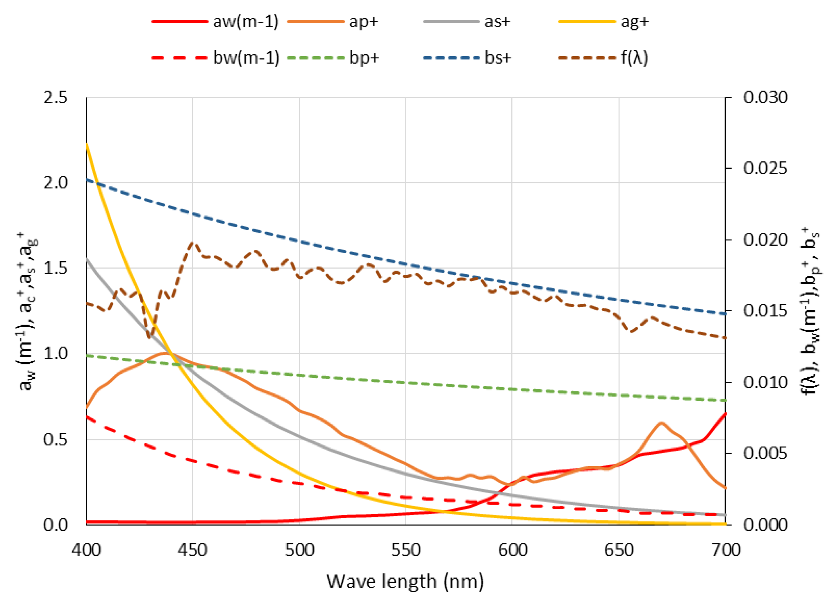
The following equations define the mathematical values for the absorption and backscattering coefficients according to the basic relationships presented in [3] for Case 1 waters. These relationships use phytoplankton chl-a concentration (μg·L−1 = mg·m−3) as a reference for the absorption relationships of phytoplankton pigment, NAPs and CDOM, as well as backscattering from phytoplankton particles and NAPs. Light absorption by phytoplankton, NAPs and CDOM uses reference absorption values of phytoplankton pigment at the wavelength λ = 440 nm, while light backscattering uses reference phytoplankton backscattering values at λ = 550 nm. Absorption coefficients for the whole visible range of the spectrum are calculated using the normalized spectral absorption values provided in the literature. Figure 2 and Table 2 present spectral distributions related to absorption by pure seawater, phytoplankton pigment, NAPs and CDOM; in addition to spectral distributions related to backscattering from phytoplankton, NAPs and seawater, as well as the derived spectral distribution function for the incident light [10].
2.1. Overall Light Attenuation
The mathematical structure of the model to calculate irradiance in oceans is similar to that presented by [10] for estuaries. The only difference is the photic depth, which defines the lower bound for irradiance in the oceans rather than the bed in shallower systems. The intensity of light at any depth can be represented by the Beer–Lambert law. The following equations summarize this model.
Beer-Lambert law:
Spectral irradiance at the bottom of the first (surface) layer:
with the incident irradiance:
and the spectral extinction coefficient:
Irradiance at the bottom of a general layer, i:
Overall irradiance for numerical integration:
where:
where E0 is the incident irradiance just beneath the water surface (W·m−2), Eℓ (W·m−2) is the irradiance at distance ℓ (m) from the incidence surface, a is the absorption coefficient (m−1), b is the scattering coefficient (m−1), E0(λ) is the spectral irradiance of the incident wavelength λ (W·m−2 nm−1) at the water surface, E1(λ) is the irradiance of wavelength λ (W·m−2·nm−1) at a downward distance ℓ1 = z1 − z0 (meters, m), K1(λ) is the extinction coefficient of the downwelling spectral irradiance (m−1) and f(λ) is the distribution function of the incident light between the various wavelengths within the PAR [10]. The subscripts w, c, s, g and p refer to water, chl-a, NAPs, CDOM (Gelbstoff) and phytoplankton, respectively; and the superscript i indicates the layer number. RRi (λj) is the reduction ratio (dimensionless) of the incident light within λj through layer ℓi. The subscript j refers to the discrete values of the normalized absorption coefficients at λj values representing PAR in 5-nm increments (j = 1–61; Table 2). According to Simpson’s rule, only half of the first and last values can be used in each summation (i.e., at j = 1 and j = 61). Introducing the 5-nm increment in Equation (6) preserves the total irradiance within the PAR. The numerical integration procedure is executed for each layer within the water column. The superscripts and subscripts are sometimes dropped for convenience. The same consistent notation is used in the following descriptions of the various attenuators at the same discrete wavelengths considering λ and λj to be synonymous.
2.1.1. Light Absorption by Pure Seawater, aw
2.1.2. Light Absorption by Algal Pigment, ac
Light absorption by phytoplankton pigment is given by the following equations [16,17]:
where ac(λ) is the absorption coefficient by phytoplankton pigment (m−1) at any wavelength λ, ac(440) is the absorption coefficient by phytoplankton pigment (m−1) at wavelength 440 nm, ac+(λ) is the normalized spectral absorption value at wavelength λ with respect to absorption at λ = 440 nm [13] and Cx,y,z,t is the concentration of chl-a (μg·L−1 = mg·m−3) at the station location, (x-eastward, y-northward), and at the layer’s vertical location z-below the water surface (m) and at the time, t, during the year. The coefficients 0.05 and 0.626 are based on observations from various regions including the North Atlantic, North Pacific, Gulf of Mexico, Mediterranean Sea, Arabian Sea and more. These coefficients can be site specific and can depend on λ [3,9,10,16]. For convenience, the stated values of the two coefficients are used in the methodology presented here. The normalized phytoplankton absorption values, ac+(λ), from Prieur and Sathyendranath [13] (Table 2) provide a consistent parameterization for the modeling methodology presented here. As expected, at the normalization wavelength, λ = 440 nm, ac+(440) = 1 (Table 2). Gallegos [18] indicated that the values of Prieur and Sathyendranath [13] are adequate for use in his bio-optical methods. The calculated value of phytoplankton absorption, ac(440), is used in the following calculations of the other absorption and backscattering coefficients.
2.1.3. Light Absorption by NAPs, as
The following equations are from IOCCG [3]:
where as(λ) is the absorption coefficient by NAPs (m−1) at any wavelength λ, as(440) is the absorption coefficient by NAPs (m−1) at wavelength 440 nm and R1 is a random value between 0.0 and 1.0. The randomness in R1 controls the random values of P1 makes the relationship between as(440) and ac(440) not fixed and avoids extremely large as(440) when ac(440) is small. The range of the random variable P1 is 0.1–0.6, and its distribution is presented in [3]. SSs is the spectral slope for NAPs (randomly valued between 0.007 and 0.015 nm−1 [3]). Recent studies indicate that the NAPs vs. the λ absorption curve has an exponential decay shape [19,20] similar to CDOM. However, understanding of the NAPs behavior is still very limited, and more detailed studies are recommended [20]. Until future values become available, this work assumes that the spectral slope for NAPs is in the middle of the above range (i.e., SSs = 0.011 nm−1). To eliminate the randomness, R1 is calibrated as presented in the Calibration and Validation Section. Values of the spectral distribution are presented in Table 2 and Figure 2.
2.1.4. Light Absorption by CDOM, ag
The following equations are from IOCCG [3]:
where ag(λ) is the absorption coefficient by CDOM (m−1) at any wavelength λ, ag(440) is the absorption coefficient by CDOM (m−1) at a wavelength of 440 nm, SSg is the spectral slope for CDOM between 0.01 and 0.02 nm−1 and R2 is a random number between 0.0 and 1.0. The randomness in R2 controls the random values of P2, makes the relationship between ag(440) and ac(440) not fixed and avoids extremely large ag(440) when ac(440) is small. The range of the random P2 values is 0.3–6.0, and its distribution is presented in [3]. To eliminate the randomness, R2 is calibrated as presented in the Calibration and Validation Section. Values of the spectral distribution are presented in Table 2 and Figure 2.
2.1.5. Light Backscattering by Phytoplankton, bp
The calculations of backscattering for phytoplankton particles include the wavelength-dependent parameters for backscattering for the whole 400–700-nm spectrum, which are based on normalized values referenced to the wavelength λ = 550 nm [3].
where is the backscattering of phytoplankton at wavelength λ, is the backscattering fraction, which depends on the phase function of phytoplankton (assumed 1% based on the Fournier-Forand phase function with respect to scattering angle [21]), P3 is randomly valued between 0.06 and 0.6 for a given Cx,y,z,t and R3 is a random value between 0.0 and 1.0. The range of the random n1 values is −0.1–2.0, and its distribution is presented in [3]. The randomness in R3 controls the random values of n1, makes the relationship between n1 and Cx,y,z,t not fixed and avoids extremely large n1 when Cx,y,z,t is small. The randomness in P3 controls the random values of and makes the relationship between and Cx,y,z,t not fixed. The range of the random values and distribution of n1 are presented in [3]. To eliminate the randomness, R3 and P3 are calibrated as presented in the Calibration and Validation Section.
The original formulation in IOCCG [3] included the extra equation (), which introduced superfluous error in bp when Cx,y,z,t was zero. This equation is not included here.
2.1.6. Light Backscattering by NAPs (Detritus, Minerals and Others), bs
Similarly, the calculations of backscattering for NAP particles include the wavelength-dependent parameters for backscattering for the whole 400–700-nm spectrum, which are based on normalized values referenced to the wavelength λ = 550 nm. The following equations are from IOCCG [3]:
where is the backscattering of NAPs at wavelength λ, is the backscattering fraction, which depends on the average particle phase function of phytoplankton (assumed 0.0183 based on the Petzold phase function with respect to scattering angle [22]), P4 is randomly valued between 0.06 and 0.6 for a given Cx,y,z,t and R4 is a random value between 0.0 and 1.0. The randomness in R4 controls the random values of n2, makes the relationship between n2 and Cx,y,z,t not fixed and avoids extremely large n2 when Cx,y,z,t is small. The randomness in P4 controls the random values of and makes the relationship between and Cx,y,z,t not fixed. The range of the random n2 values is −0.2–2.2, and its distribution is presented in [3]. To eliminate the randomness, R4 and P4 are calibrated as presented in the Calibration and Validation Section. Examples of the values of the spectral distribution for an arbitrary chl-a concentration are presented in Table 2 and Figure 2. These values will change with depth according to the chl-a concentration (Equation (21)).
2.1.7. Light Backscattering by Pure Seawater, bw
2.2. Data
Existing irradiance and chl-a data from the North Atlantic were used to calibrate and validate the presented methodology. Data were obtained through personal communication [24]. Details of the field methods, protocols and times are published in [25], and they are not repeated here. The data included incident surface irradiance (W·m−2) at the water surface for all wavelengths within PAR at 5-nm increments, profiles of the downwelling irradiance (W·m−2) at 2 m-depth increments and chl-a concentration profiles at various depth locations during various seasons. The data indicated that chl-a concentrations were always <3.5 μg·L−1. Data analysis indicated that the ship-based and the glider-based surface PAR agree [25]. Accordingly, the glider surface records were used here to represent the incident irradiance for the remainder of the corresponding downwelling profile.
Two sets of consistent data of incident irradiance, irradiance profile and chl-a profile were used to calibrate and validate the presented methodology. The major criteria to choose these data were: cloud cover does not obstruct incident irradiance during the period 10:00 GMT–14:00 GMT; the chl-a profile measurements are collected on the same day of the irradiance data; and the data extend to at least 100 m below the water surface. The collected chl-a concentrations were sparse throughout the monitored top part of the water column and had to be interpolated at the same depth increments as the irradiance profile (i.e., 2 m). Only fourteen chl-a data profiles reached depths ≥100 m. Two of these profiles with contrasting vertical distributions were used here.
2.2.1. The Spectrum Shape Function, f
For modeling purposes, Abdelrhman [10] suggested the use of the spectrum shape function at the top of the atmosphere to redistribute the incident irradiance, E0, to its spectral values, E0(λ), within the PAR at the water surface (Table 2). The spectrum shape function alleviates the need to identify E0(λ) at each location throughout the simulation time. Instead, the overall incident irradiance, E0, can be used with f(λ) (Equation (3)). This simplification is tested with the incident irradiance of 339 W·m−2 on 11 June 2013 at 9:30 GMT. Figure 3a compares the shapes of the actual incident irradiance to that of the shape function, f(λ) (Table 2). The difference between the calculated and observed values is ±5% for most of the PAR (λ = 450 nm–650 nm) and <±15% outside that range. The scatter plot (Figure 3b) indicates that the correlation (slope) between calculated and observed shapes is 0.9981 (R2 = 0.7068) with zero intercept, which indicates that the use of f(λ) is adequate for modeling purposes. The spectrum shape function is used here to define the spectral distribution for the topmost near-surface record of the downwelling irradiance profile.
2.2.2. The Summer Dataset
The summer data used in this study were collected on 11 June 2013 (Figure 4). The concentration of chl-a showed a systematically decreasing trend with depth below the water surface (Figure 4a). This trend was used to calculate chl-a concentrations at 2 m-depth increments, which correspond to the measurements of the downwelling irradiance. The average of four irradiance profiles collected during midday (10:00 GMT–14:00 GMT) was used to represent the observed downwelling irradiance, E, on that day (Figure 4b). The topmost irradiance value was assumed to represent the incident irradiance, E0. The distribution of the incident PAR was reconstructed according to Equation (3) (Figure 4c).
2.2.3. The Fall Data Set
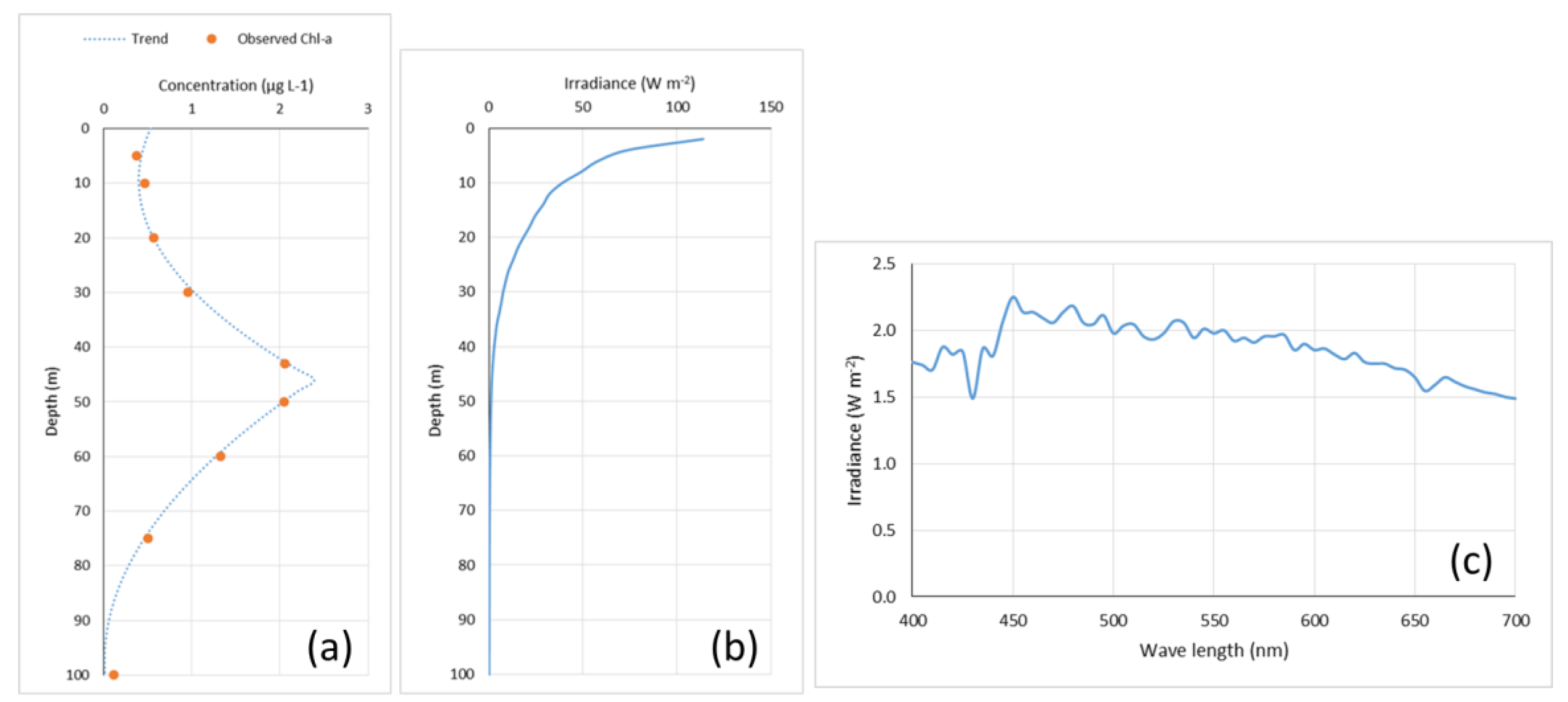
A subsurface maximum of chl-a concentration appeared in the fall season of 2013 at ~30–40 m below the water surface [25]. The data on 3 September 2013 consisted of the chl-a profile (Figure 5a), which demonstrated the subsurface maximum chl-a concentration. Two trends were used to interpolate chl-a concentrations at 2-m increments corresponding to the measured downwelling irradiance. The average of four irradiance profiles collected during midday (10:00 GMT–14:00 GMT) was used to represent the observed downwelling irradiance, E, on that day (Figure 5b). The topmost irradiance value was assumed to represent the incident irradiance, E0. The distribution of the incident PAR was reconstructed according to Equation (3) (Figure 5c).
2.3. Calibration and Validation
The following three important rules of thumb were observed in calibration: (1) any attenuation coefficient for any contributor at any wavelength (i.e., the exponentiation terms in Equations (5)–(7)) cannot exceed 1.0 at any depth; (2) any attenuation coefficient for any contributor except water should be correlated with chl-a concentration (the surrogate for all attenuations); and (3) observed irradiance should not exceed the irradiance in pure seawater.
2.3.1. Calibration with Fall Data
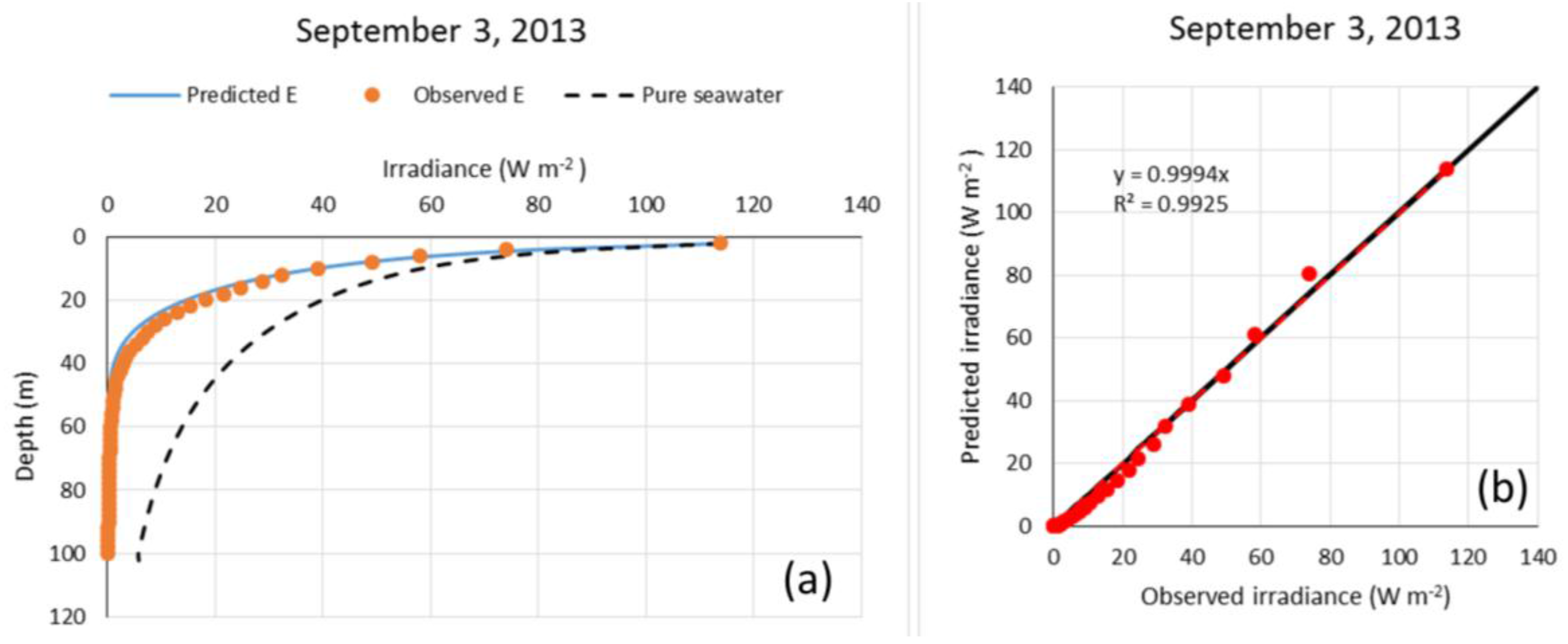
The main purpose of the calibration is to define non-random (fixed) values for R1, R2, R3, R4, P3 and P4. The measured topmost value of the downwelling irradiance represented E0 on 3 September 2013; the recorded light intensity at each depth represented Eℓ; depth increments (2 m) represented the layer thickness, ℓ; and the interpolated chl-a concentration within each layer represented Cx,y,z,t. The calibration started with the mid-range values of the parameter and proceeded to improve the fit with observations of the downwelling irradiance to find the correlation between predicted and observed values. A zero intercept was enforced in all of the correlation plots. For convenience, the p-values were assumed to be the same within their range of 0.06–0.6 (range = 0.54), and the R values were also assumed to be the same within their specified range of 0.0–1.0 (range = 1.0). Both p and R ranges were divided into 10 increments. Systematic iterations took place by fixing the p-values at each of the incremented values and checking the correlation between predicted and observed irradiances at each of the R incremented values. Figure 6a presents the calibrated irradiance profile with all of the R parameters calibrated to 0.3 and the p parameters calibrated to 0.438. The correlation scatter plot (Figure 6b) indicates that the calculated irradiance agreed with observed values (R2 = 0.9925). The regression line slope was 0.9994, which is very close to unity for a one-to-one correlation.
2.3.2. Validation with Summer Data
Using the same calibration values for the R and p parameters, the summer irradiance profile on 11 June 2013 was checked against observations (Figure 7a). The scatter plot showed weaker linear agreement with the r2 value of 0.8497 (Figure 7b). The regression line slope with zero intercept was 0.709, which reflects a one to-one correlation between predicted and observed profiles. The reason for the lower correlation was attributed to other factors (e.g., stratification). In addition, the reported irradiance measurements within the top 12 m coincided with the values of pure seawater (Figure 7a), which un-intuitively does not represent effects from other attenuators. Validation with other data is needed (see the discussion).
3. Results
The following results present a sample to illustrate the availability and quality of light in ocean waters. The availability of light is defined by the photic depth at which 1% of the incident irradiance exists. In addition, the presented methodology can identify the various depths where the spectral values reach 1% of their incident values. As some spectral bands will become extinct before others, the quality of light refers to the amount of energy remaining in each spectral band at any depth.
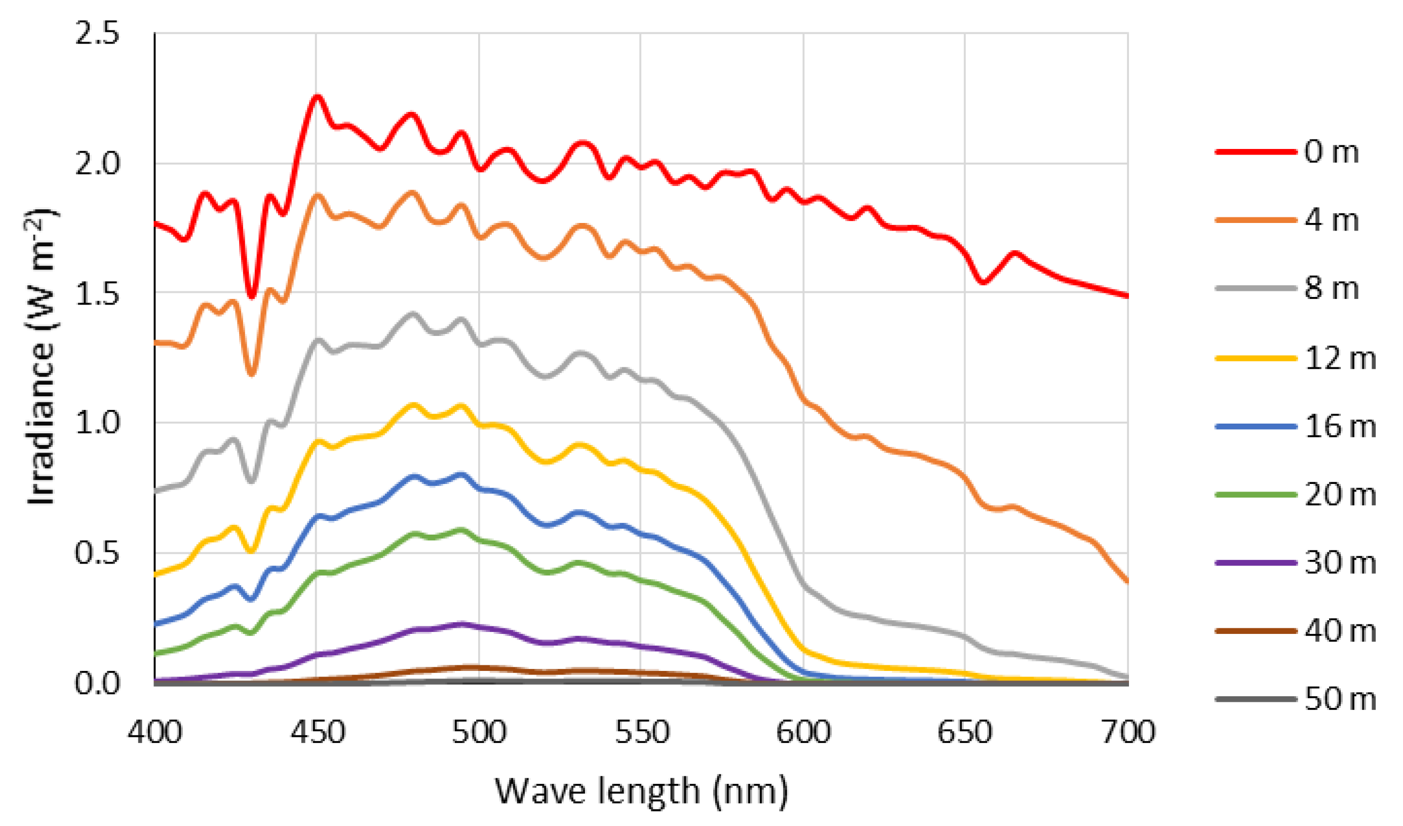
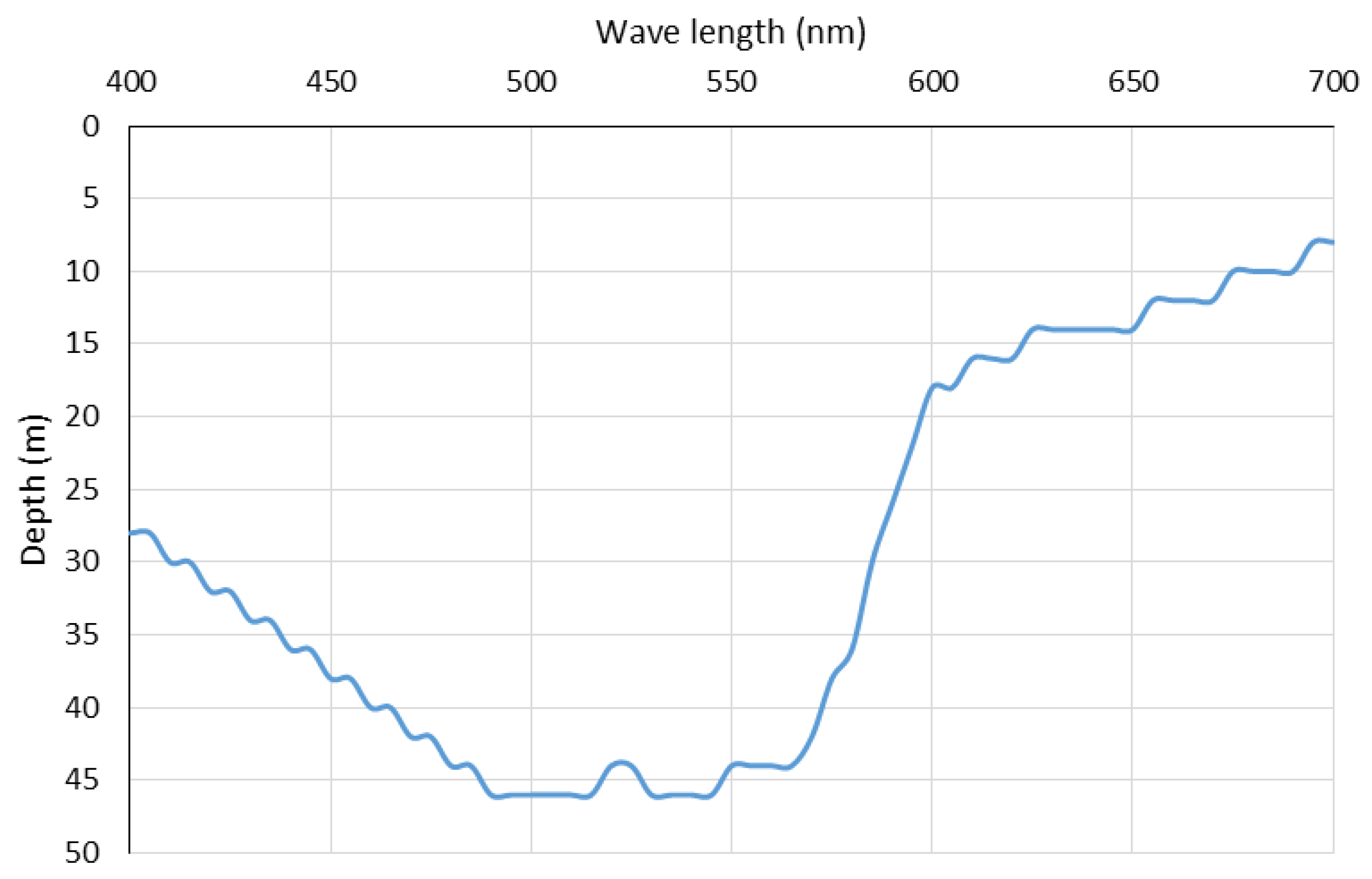
Figure 8 presents the percent change in the total downwelling irradiance with depth, which indicates a photic depth of 50 m on 3 September 2013. Figure 9 presents the penetration profiles of various wavelengths. The high wavelengths are attenuated heavily within the top 10–20 m, while the shorter wavelengths continue to deeper waters. The penetration depths of the whole PAR on the same day are shown in Figure 10. Wavelengths 485–500 nm reached a maximum depth of 46 m, while those close to 700 nm were almost extinct at an 8-m depth. Figure 11 presents the change in the spectral distribution of the PAR throughout the water column, which defines the light quality on that day. It is worth recalling that the shape and penetration depth of the various wavelengths will change throughout space and time as the chl-a concentration and incident irradiance change.
4. Discussion
A mathematical approach was presented to calculate irradiance in ocean waters (Case 1 waters). The methodology is not site-specific, and it can be applied to any system. Nevertheless, proper calibration of the bio-optical model remains an essential factor for any site-specific application. The methodology presented here utilized relationships from a wide range of absorption and backscattering spectra that were presented by the IOCCG [3]. This range was based on mathematical relationships that used phytoplankton concentration in ocean waters as a reference to estimate all absorption and backscattering components in the water column. Employing numerical modeling with bio-optical modeling validates the use of the presented approach for predictions of future scenarios related to changes in environmental and anthropogenic conditions. For example, environmental impacts due to global warming may cause alterations to seasonal cycles in temperature, precipitation and wind patterns. Such alterations can impact ocean circulation and stratification, which directly impacts the transport, distribution and composition of phytoplankton groups and consequently their optical properties. Similarly, anthropogenic effects due to increased aerosols can alter the incident light, which affects the photic depth and the wellbeing of the phytoplankton communities.
It is argued here that the photic depth (at 1% irradiance) is an aggregate parameter for phytoplankton studies and that a more detailed representation of the “light quality” is more appropriate. As presented above, while the photic depth was 50 m, some wavelengths were extinct in much shallower depths (Figure 10). The resolved PAR distribution with depth (i.e., Figure 11) identifies light quality throughout the water column, which can provide useful information about the wellbeing of the phytoplankton communities at various depths. Such information can help in studies of primary productivity in the oceans. Most current numerical models calculate production (photosynthesis) based on total PAR only. In order for light quality to affect numerical models, they must compute the spectral photosynthesis of the competing dominant phytoplankton species and their adaptation to irradiance throughout the photic depth. An example of the complexity in this area is tackled for two coexisting phytoplankton species in [26]. Partial numerical implementation was presented using λ = 490 nm as a proxy to the PAR [27]. This topic needs more future studies to provide further guidance for implementing light quality and spectral photosynthesis in such models.
As indicated in the presented methodology, calibration is essential to reduce the level of uncertainty in the final irradiance predictions. Calibration of the bio-optical models eliminated the random processes that were incorporated in the original formulation [3]. Constant values for the relevant mathematical parameters and coefficients were calibrated using field observations [24]. The two physical parameters in Equation (9) can be site specific [3] and may have to be included in the calibration. Similarly, the spectral slopes (Equations (10) and (13)) have to be defined properly. Allowing such parameters to vary requires proper coupling between light and phytoplankton to account for the continually-changing parameterization (see the proposed numerical steps below). Validation of the presented methodology requires consistent high quality sets of data from various locations during various seasons. Figure 7 indicates that the observed downwelling irradiance failed to capture the attenuation within the top 12 m, which had the highest observed chl-a concentrations in the profile (Figure 4). Such inconsistency infers an unjustified increase in the observed downwelling irradiance. While physical effects (e.g., from density stratification) are beyond the scope of this work, they may have impacted the model and data shown. More data are definitely needed to improve the calibration and validation of the presented approach.
There are two major implications of the presented methodology: modeling implications and ecological implications. The methodology presented validates the coupling of bio-optical models with three-dimensional water quality models. The numerical implications of coupling phytoplankton to light in water quality models can execute the following general steps, which are recommended for relevant future work:
- At time t
- At location x,y
- For layer ℓi
- The numerical model provides Cx,y,z,t
- Calculate ac(440) (Equation (9))
- For every wavelength, calculate: ac(λ), as(λ), ag(λ), bp(λ), bs(λ) (Equations (8), (10), (13), (16) and (19), respectively)
- Calculate the spectral attenuation coefficient, Ki(λ), for each λ (Equation (4))
- Calculate attenuated irradiance for each λ, Ei(λ) (Equation (5))
- Calculate total irradiance, Ei, by numerical integration over all λ (Equation (6))
- Move to the next layer down (i + 1) and repeat Steps 4–9
- Move to next location and repeat Steps 3–10
- For each layer, use Ei in the calculation of Cx,y,z,t+Δt, which fully couples light and phytoplankton at the next time level (t + Δt).
The ecological implications encompass the predictive ability of phytoplankton biomass and its primary productivity in the oceans. Coupling light quality to water quality models facilitates understanding the relationship between light quality and phytoplankton. Light quality impacts the composition and health of phytoplankton communities in the water column, which, consequently, alter water clarity and irradiance levels. Water clarity is a major indicator used for many management decisions related to the health of estuarine, coastal and ocean waters. To the author’s knowledge, such coupling is not present in most water quality models. However, recently, it was implemented in studies of primary productivity in the Pacific Ocean [27].
The presented approach is expected to work well in environments where phytoplankton particles are the major contributor to light attenuation through absorption by their chl-a pigment, their dead NAPs cells and their exudation of CDOM; as well as backscattering by the particulate phytoplankton cells and their dead NAPs. In other environments (e.g., with density stratification), the approach has to be augmented with additional considerations to account for such effects. Processes related to phytoplankton composition and dynamics (e.g., transport and vertical migration) should be covered by the water quality model. As the methodology is based on chl-a concentration, situations when phytoplankton cells and their chl-a content change may pose a challenge to this approach.
5. Conclusions
Predictive numerical models can use the presented methodology to couple light with phytoplnkton physiology throughout the photic depth. Not only light quantity but also its quality are essentisl for proper coupling. Nonetheless, numerical models have to accommodate the spectral photosynthesis of the competing dominant phytoplankton species and their adaptation to the spectral irradiance throughout the photic depth. The complexity of this coupling is still unresolved and needs more attention from both the numerical modeling community as well as the optical and bio-optical scientists.
Acknowledgments
The author wishes to thank Victoria S. Hemsley (Ocean and Earth Science, National Oceanography Center Southampton, University of Southampton, SO14 3ZH, U.K.) for providing all of the field data. The author also thanks the in-house reviewers of this manuscript, including Dan Campbell, Naomi Detenbeck and Henry Walker (USEPA-AED), as well as the journal’s anonymous reviewers for their technical reviews, insights and constructive comments. Although the research described here has been funded by the U.S. Environmental Protection Agency, it has not been subject to agency-level review and, therefore, does not necessarily reflect the views of the agency, nor does mentioning trade names or commercial products endorse or recommend them. This manuscript is contribution No. ORD-017268 of the USEPA Office Research and Development, National Health and Environmental Effects Research Laboratory, Atlantic Ecology Division.
Conflicts of Interest
The author declares no conflict of interest.
References
- Peterson, D.H.; Festa, J.F. Numerical simulation of phytoplankton productivity in partially mixed estuaries. Estuar. Coast. Shelf Sci. 1984, 19, 563–589. [Google Scholar] [CrossRef]
- Topliss, B.J. Optical monitoring of coastal waters: Photic depth estimates. Mar. Environ. Res. 1982, 7, 295–308. [Google Scholar] [CrossRef]
- Ocean Color Algorithm Working Group. Models, Parameters and Approaches That Are Used to Generate Wide Range of Absorption and Backscattering Spectra. International Ocean Color Coordinating Group, Ocean Color Algorithm Working Group. 2003, p. 11. Available online: http://www.ioccg.org/groups/lee_data.pdf (accessed on 30 July 2015).
- Gallegos, C.L.; Kenworthy, W.J. Seagrass depth limits in the Indian River Lagoon (Florida, USA): Application of an optical water quality model. Estuar. Coast. Shelf Sci. 1996, 42, 267–288. [Google Scholar] [CrossRef]
- Gallegos, C.L. Calculating optical water quality targets to restore and protect submerged aquatic vegetation: Overcoming problems in partitioning the diffuse attenuation coefficient for photosynthetically active radiation. Estuaries 2001, 24, 381–397. [Google Scholar] [CrossRef]
- Gallegos, C.L.; Neal, P.J. Partitioning spectral absorption in case 2 waters: Discrimination of dissolved and particulate components. Appl. Opt. 2002, 41, 4220–4233. [Google Scholar] [CrossRef] [PubMed]
- Keith, D.J.; Yoder, J.A.; Freeman, S.A. Spatial and temporal distribution of colored dissolved organic matter (CDOM) in Narragansett Bay, Rhode Island: Implications for phytoplankton in coastal waters. Estuar. Coast. Shelf Sci. 2002, 55, 705–717. [Google Scholar] [CrossRef]
- Kenworthy, W.J.; Gallegos, C.L.; Costello, C.; Field, D.; di Carlo, G. Dependence of eelgrass (Zostera marina) light requirements on sediment organic matter in Massachusetts coastal bays: Implications for remediation and restoration. Mar. Pollut. Bull. 2014, 83, 446–457. [Google Scholar] [CrossRef] [PubMed]
- Thursby, G.; Rego, S.; Keith, D. Data Report for Calibration of Bio-Optical Model for Narragansett Bay; United States Environmental Protection Agency Report Tracking Number EPA/600/R-15/211; U.S. Environmental Protection Agency: Washington, DC, USA, 2015; p. 25. Available online: https://cfpub.epa.gov/si/si_public_file_download.cfm?p_download_id=525010 (Accessed on 11 November 2016).
- Abdelrhman, M.A. Quantifying contributions to light attenuation in estuaries and coastal embayments: Application to Narragansett Bay, Rhode Island. Estuar. Coasts, 13 April 2016; under review. [Google Scholar]
- Morel, A. Optical modeling of the upper ocean in relation to its biogenous matter content (Case I Waters). J. Geophys. Res. 1988, 93, 10749–10768. [Google Scholar] [CrossRef]
- Sathyendranath, S.; Platt, T. The spectral irradiance field at the surface and in the interior of the ocean: A model for applications in oceanography. J. Geophys. Res. 1988, 93, 9270–9280. [Google Scholar] [CrossRef]
- Prieur, L.; Sathyendranath, S. An optical classification of coastal and oceanic waters based on the specific spectral absorption curves of phytoplankton pigment, dissolved organic matter, and other particulate materials. Limnol. Oceanogr. 1981, 26, 671–689. [Google Scholar] [CrossRef]
- Jerlov, N.G. Marine Optics. In Elsevier Oceanography Series 14; Elsevier: New York, NY, USA, 1976; p. 231. [Google Scholar]
- Sathyendranath, S. Inherent optical properties of natural seawater. Defense Sci. J. 1984, 34, 1–18. [Google Scholar] [CrossRef]
- Bricaud, A.; Babin, M.; Morel, A.; Claustre, H. Variability in chlorophyll-specific absorption coefficients of natural phytoplankton: Analysis and parameterization. J. Geophys. Res. 1995, 100, 13321–13332. [Google Scholar] [CrossRef]
- Fischer, J.; Fell, F. Simulation of MERIS measurements above selected ocean waters. Int. J. Remote Sens. 1999, 20, 1787–1807. [Google Scholar] [CrossRef]
- Gallegos, C.L. Refining habitat requirements of submersed aquatic vegetation: Role of optical models. Estuaries 1994, 17, 187–199. [Google Scholar] [CrossRef]
- Bricaud, A.; Stramski, D. Spectral absorption coefficients of living phytoplankton and nonalgal biogenous matter: A comparison between the Peru upwelling area and the Sargasso Sea. Limnol. Oceanogr. 1990, 35, 562–582. [Google Scholar] [CrossRef]
- Matsuoka, A.; Hill, V.; Hout, Y.; Babin, M.; Bricaud, A. Seasonal variability in the light absorption properties of western Arctic waters: Parameterization of individual components of absorption for ocean color applications. J. Geophys. Res. 2011, 116, 1–15. [Google Scholar] [CrossRef]
- Fournier, G.; Forand, J.L. Analytic phase function for ocean water. In Ocean Optics XII, Proceedings of SPIE—The International Society for Optical Engineering XII, Bergen, Norway, 13–15 June 1994; Jaffe, J.S., Ed.; Society of Photo-optical Instrumentation Engineers: Bellingham, WA, USA, 1994; Volume 2258, pp. 194–201. [Google Scholar]
- Morel, A.; Gentili, B. Diffuse reflectance of oceanic waters: Its dependence on sun angle as influenced by molecular scattering contribution. Appl. Opt. 1991, 30, 4427–4438. [Google Scholar] [CrossRef] [PubMed]
- Buiteveld, H.; Hakvoort, J.H.M.; Donze, M. The optical properties of pure water. In Ocean Optics XII, Proceedings of SPIE—The International Society for Optical Engineering XII, Bergen, Norway 13–15 June 1994; Jaffe, J.S., Ed.; Society of Photo-optical Instrumentation Engineers: Bellingham, WA, USA, 1994; Volume 2258, pp. 174–183. [Google Scholar]
- Hemsley, V.S.; University of Southampton, Southampton, UK. Personal communication, 2016.
- Hemsley, V.S.; Smyth, T.J.; Martin, A.P.; Williams, E.F.; Thompson, A.F.; Damerell, G.; Painter, S.C. Estimating oceanic primary production using vertical irradiance and chlorophyll profiles from ocean gliders in the North Atlantic. Environ. Sci. Technol. 2015, 49, 11612–11621. [Google Scholar] [CrossRef] [PubMed] [Green Version]
- Stomp, M.; Huisman, J.; de Jongh, F.; Veraart, A.J.; Gerla, D.; Rijkeboer, M.; Ibelings, B.W.; Wollenzien, U.I.A.; Stal, L.J. Adaptive divergence in pigment composition promotes phytoplankton biodiversity. Nature 2004, 432, 104–107. [Google Scholar] [CrossRef] [PubMed]
- Xiu, P.; Chai, F. Connections between physical, optical, and biogeochemical processes in the Pacific Ocean. Prog. Oceanogr. 2014, 122, 30–53. [Google Scholar] [CrossRef]
Figure 1.
Definition sketch of the relation between the numerical model vertical structure and its utilization to study light intensity throughout the water column. Concentration of chl-a (Cx,y,z,t) should be provided by the numerical model at location (x,y) at every layer depth (z) and at every time step (t) during the year. Ei−1 and Ei are the incident and departing downwelling irradiances through layer i (with thickness ℓi and extinction coefficient Ki) (Table 1).

Figure 2.
Spectral distributions of absorption by pure water and the normalized absorption coefficients for phytoplankton pigment, NAPs and CDOM (full lines read on left axis); in addition to backscattering from phytoplankton, NAPs and water, as well as the derived spectral distribution function for the incident light (broken lines read on right axis). Refer to Table 2 for the definitions of normalized absorption and backscattering coefficients.

Figure 3.
Comparison between observed and reconstructed spectrum shape functions on 11 June 2013 at 9:30 a.m.: (a) spectral distributions and the % error (100 (observed-calculated)/observed); (b) correlation between observed and calculated spectral values.
Figure 3.
Comparison between observed and reconstructed spectrum shape functions on 11 June 2013 at 9:30 a.m.: (a) spectral distributions and the % error (100 (observed-calculated)/observed); (b) correlation between observed and calculated spectral values.
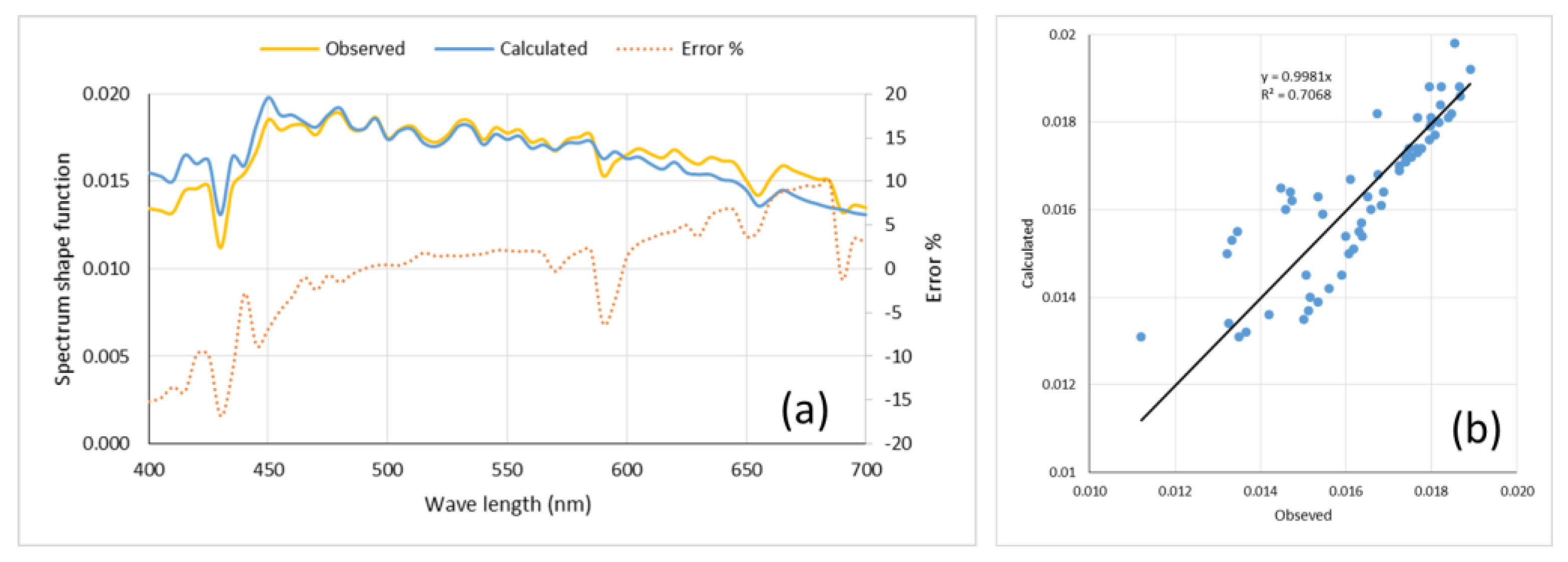
Figure 4.
Summer data on 11 June 2013: (a) vertical distribution of ship-based measurements of chl-a concentrations and their vertical trend; (b) vertical distribution of glider-based average irradiance from 10:00 GMT-14:00 GMT; (c) spectral distribution of the near-surface average irradiance measurement.
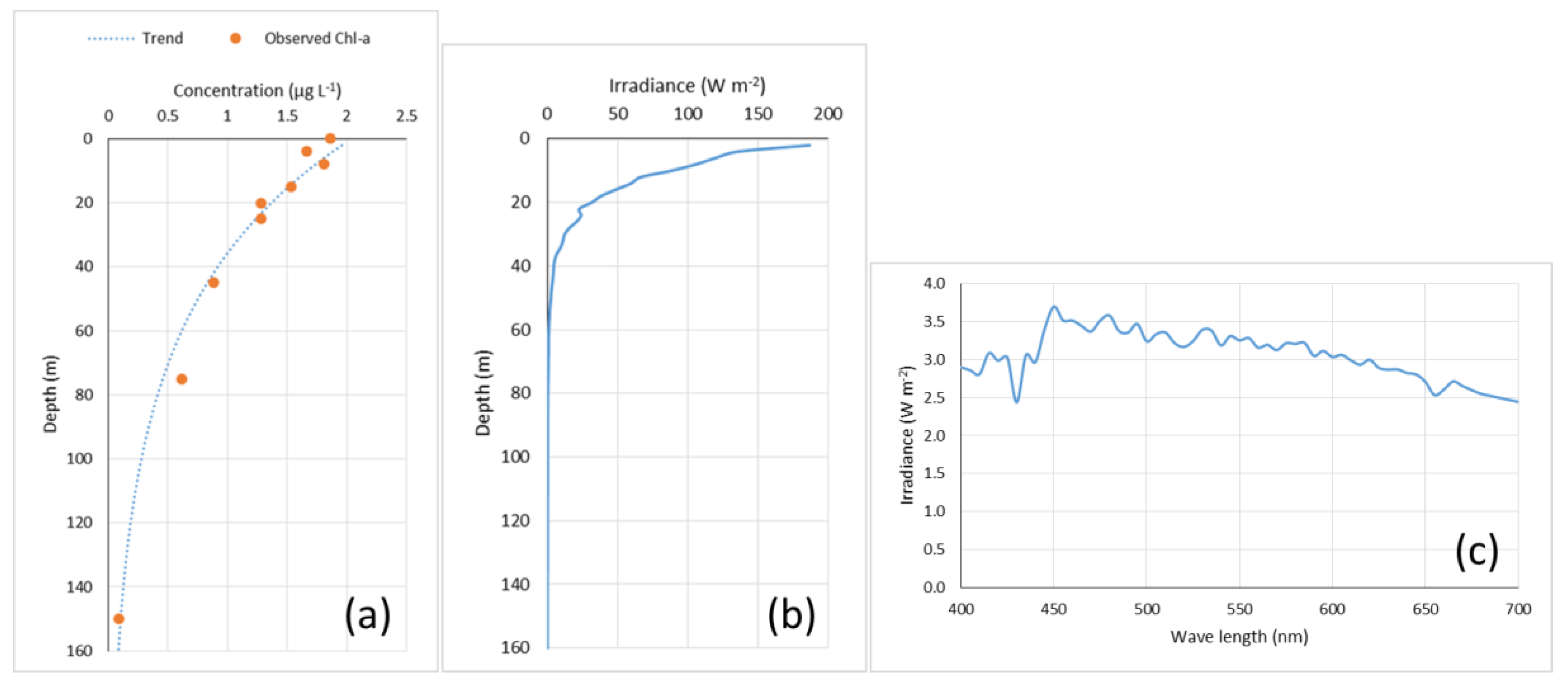
Figure 5.
Fall data on 3 September 2013: (a) vertical distribution of ship-based measurements of chl-a concentrations and their vertical trend; (b) vertical distribution of glider-based average irradiance from 10:00 GMT-14:00 GMT; (c) spectral distribution of the near-surface average irradiance measurement.

Figure 6.
Calibration using fall data: (a) comparison between observed and predicted vertical irradiance profiles together with the expected irradiance in pure seawater; (b) correlation between observed and predicted irradiances.
Figure 6.
Calibration using fall data: (a) comparison between observed and predicted vertical irradiance profiles together with the expected irradiance in pure seawater; (b) correlation between observed and predicted irradiances.

Figure 7.
Validation using summer data: (a) comparison between observed and predicted vertical irradiance profiles together with the expected irradiance in pure seawater; (b) correlation between observed and predicted irradiances.
Figure 7.
Validation using summer data: (a) comparison between observed and predicted vertical irradiance profiles together with the expected irradiance in pure seawater; (b) correlation between observed and predicted irradiances.
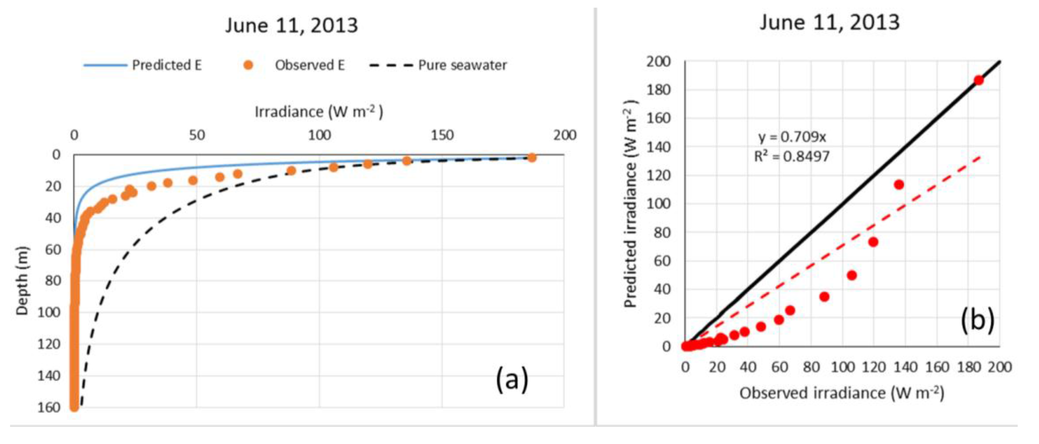
Figure 8.
Change of the total downwelling irradiance with depth on 3 September 2013.
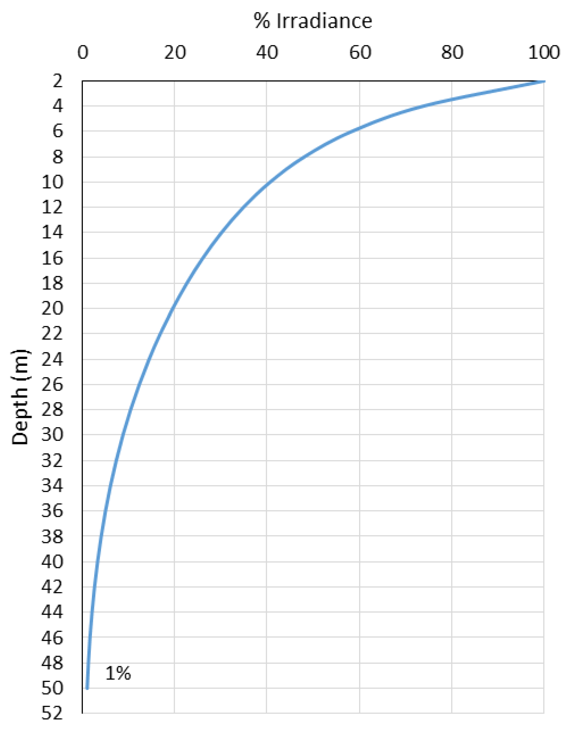
Figure 9.
Profiles and penetrations of various wavelengths, which illustrates the change in light quality with depth.
Figure 9.
Profiles and penetrations of various wavelengths, which illustrates the change in light quality with depth.
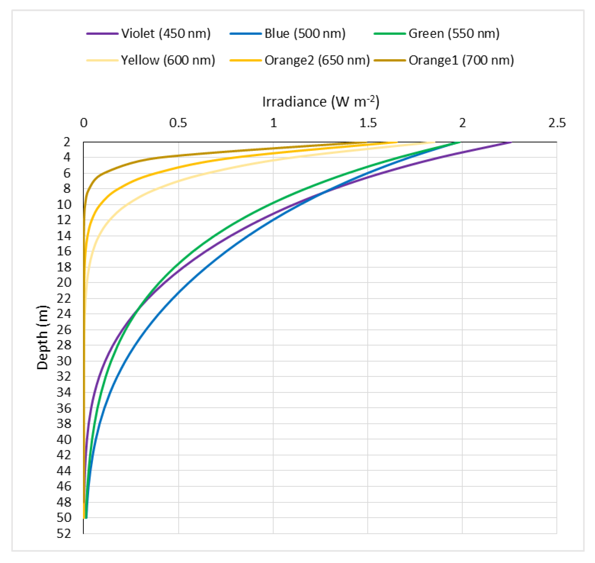
Figure 10.
Penetration depth of the PAR on 3 September 2013.

Figure 11.
Change of the spectral distribution of the PAR throughout the water column on 3 September 2013.
Figure 11.
Change of the spectral distribution of the PAR throughout the water column on 3 September 2013.

| Symbol | Definition | Dimension |
|---|---|---|
| Abbreviations | ||
| CDOM | Colored dissolved organic material | |
| chl-a | Chlorophyll a | |
| IOCCG | International Ocean Color Coordination Group | |
| NAPs | Non-algal particles | |
| PAR | Photosynthetically-available radiation | |
| TSS | Total suspended solids | |
| Parameters | ||
| aw | Absorption coefficient of seawater | m−1 |
| ac | Absorption coefficient of chl-a | m−1 |
| as | Absorption coefficient of NAPs | m−1 |
| ag | Absorption coefficient of CDOM | m−1 |
| bw | Backscattering a coefficient of seawater | m−1 |
| bp | Backscattering a coefficient of phytoplankton particles | m−1 |
| bs | Backscattering a coefficient of NAPs | m−1 |
| C | chl-a concentration | μg·L−1 |
| E0 | Irradiance at the water surface | W·m−2 |
| Ei, Eℓ | Irradiance at the bottom of the i-th layer, ℓi | W·m−2 |
| e | Exponentiation base (e = 2.718281828459) | dimensionless |
| f | Spectrum distribution function | dimensionless |
| g | CDOM concentration (not implemented) | μg·L−1 |
| K | Downwelling a extinction coefficient | m−1 |
| ℓi | Layer thickness (zi − zi−1) | m |
| P3,4 | Calibration coefficients | dimensionless |
| R1,2,3,4 | Calibration coefficients | dimensionless |
| RRi(λj) | Reduction ratio of wavelength λj at the i-th layer | dimensionless |
| S | NAPs concentration | mg·L−1 |
| SS | Spectral slope | nm−1 |
| λ | Wavelength | nm |
| Subscripts | ||
| i | Counter for the water layer, | |
| j | Counter for the wavelength λ | |
| t | Time | |
| x | Eastward spatial location (see Figure 1) | |
| y | Northward spatial location (see Figure 1) | |
| z | Vertical spatial location below the water surface (see Figure 1) | |
| Superscripts | ||
| + | Normalized value (see Table 2 and Figure 2) | |
a To avoid confusion in the subscripts presented in various equations, b is used for backscattering instead of the commonly used bb, and K is used instead of Kd for the downwelling extinction coefficient.
Table 2.
Spectral distributions of absorption, a, backscattering, b, and the shape function, f, for the PAR (see the footnotes for details).
| 1 | 2 | 3 | 4 | 5 | 6 | 7 | 8 | 9 | 10 |
|---|---|---|---|---|---|---|---|---|---|
| i | λi | aw (m−1) | bw (m−1) | f(λ) | |||||
| 1 | 400 | 0.0180 | 0.6870 | 1.5530 | 2.2260 | 0.0076 | 1.1890 | 1.3250 | 0.0155 |
| 2 | 405 | 0.0180 | 0.7810 | 1.4700 | 2.0140 | 0.0072 | 1.1810 | 1.3100 | 0.0153 |
| 3 | 410 | 0.0170 | 0.8280 | 1.3910 | 1.8220 | 0.0068 | 1.1730 | 1.2960 | 0.0150 |
| 4 | 415 | 0.0170 | 0.8830 | 1.3170 | 1.6490 | 0.0065 | 1.1650 | 1.2820 | 0.0165 |
| 5 | 420 | 0.0160 | 0.9130 | 1.2460 | 1.4920 | 0.0061 | 1.1580 | 1.2690 | 0.0160 |
| 6 | 425 | 0.0160 | 0.9390 | 1.1790 | 1.3500 | 0.0058 | 1.1500 | 1.2560 | 0.0162 |
| 7 | 430 | 0.0150 | 0.9730 | 1.1160 | 1.2210 | 0.0055 | 1.1430 | 1.2430 | 0.0131 |
| 8 | 435 | 0.0150 | 1.0010 | 1.0570 | 1.1050 | 0.0052 | 1.1360 | 1.2300 | 0.0164 |
| 9 | 440 | 0.0150 | 1.0000 | 1.0000 | 1.0000 | 0.0049 | 1.1290 | 1.2180 | 0.0159 |
| 10 | 445 | 0.0150 | 0.9710 | 0.9460 | 0.9050 | 0.0047 | 1.1220 | 1.2060 | 0.0182 |
| 11 | 450 | 0.0150 | 0.9440 | 0.8960 | 0.8190 | 0.0045 | 1.1150 | 1.1940 | 0.0198 |
| 12 | 455 | 0.0160 | 0.9280 | 0.8480 | 0.7410 | 0.0043 | 1.1080 | 1.1820 | 0.0188 |
| 13 | 460 | 0.0160 | 0.9170 | 0.8030 | 0.6700 | 0.0041 | 1.1020 | 1.1710 | 0.0188 |
| 14 | 465 | 0.0160 | 0.9020 | 0.7600 | 0.6070 | 0.0039 | 1.0950 | 1.1600 | 0.0184 |
| 15 | 470 | 0.0160 | 0.8700 | 0.7190 | 0.5490 | 0.0037 | 1.0890 | 1.1490 | 0.0181 |
| 16 | 475 | 0.0170 | 0.8390 | 0.6800 | 0.4970 | 0.0036 | 1.0830 | 1.1380 | 0.0188 |
| 17 | 480 | 0.0180 | 0.7980 | 0.6440 | 0.4490 | 0.0034 | 1.0770 | 1.1280 | 0.0192 |
| 18 | 485 | 0.0190 | 0.7730 | 0.6100 | 0.4070 | 0.0033 | 1.0710 | 1.1170 | 0.0181 |
| 19 | 490 | 0.0200 | 0.7500 | 0.5770 | 0.3680 | 0.0031 | 1.0650 | 1.1070 | 0.0180 |
| 20 | 495 | 0.0230 | 0.7170 | 0.5460 | 0.3330 | 0.0030 | 1.0590 | 1.0970 | 0.0186 |
| 21 | 500 | 0.0260 | 0.6680 | 0.5170 | 0.3010 | 0.0029 | 1.0530 | 1.0880 | 0.0174 |
| 22 | 505 | 0.0310 | 0.6450 | 0.4890 | 0.2730 | 0.0028 | 1.0470 | 1.0780 | 0.0179 |
| 23 | 510 | 0.0360 | 0.6180 | 0.4630 | 0.2470 | 0.0026 | 1.0420 | 1.0690 | 0.0180 |
| 24 | 515 | 0.0420 | 0.5820 | 0.4380 | 0.2230 | 0.0025 | 1.0360 | 1.0600 | 0.0172 |
| 25 | 520 | 0.0480 | 0.5280 | 0.4150 | 0.2020 | 0.0024 | 1.0310 | 1.0510 | 0.0170 |
| 26 | 525 | 0.0500 | 0.5040 | 0.3930 | 0.1830 | 0.0023 | 1.0260 | 1.0420 | 0.0174 |
| 27 | 530 | 0.0510 | 0.4740 | 0.3720 | 0.1650 | 0.0022 | 1.0200 | 1.0330 | 0.0182 |
| 28 | 535 | 0.0540 | 0.4440 | 0.3520 | 0.1500 | 0.0022 | 1.0150 | 1.0250 | 0.0181 |
| 29 | 540 | 0.0560 | 0.4160 | 0.3330 | 0.1350 | 0.0021 | 1.0100 | 1.0160 | 0.0171 |
| 30 | 545 | 0.0600 | 0.3840 | 0.3150 | 0.1220 | 0.0020 | 1.0050 | 1.0080 | 0.0177 |
| 31 | 550 | 0.0640 | 0.3570 | 0.2980 | 0.1110 | 0.0019 | 1.0000 | 1.0000 | 0.0174 |
| 32 | 555 | 0.0680 | 0.3210 | 0.2820 | 0.1000 | 0.0019 | 0.9950 | 0.9920 | 0.0176 |
| 33 | 560 | 0.0710 | 0.2940 | 0.2670 | 0.0910 | 0.0018 | 0.9900 | 0.9840 | 0.0169 |
| 34 | 565 | 0.0760 | 0.2730 | 0.2530 | 0.0820 | 0.0018 | 0.9860 | 0.9770 | 0.0171 |
| 35 | 570 | 0.0800 | 0.2760 | 0.2390 | 0.0740 | 0.0017 | 0.9810 | 0.9690 | 0.0168 |
| 36 | 575 | 0.0940 | 0.2680 | 0.2270 | 0.0670 | 0.0017 | 0.9760 | 0.9620 | 0.0172 |
| 37 | 580 | 0.1080 | 0.2910 | 0.2140 | 0.0610 | 0.0016 | 0.9720 | 0.9540 | 0.0172 |
| 38 | 585 | 0.1330 | 0.2740 | 0.2030 | 0.0550 | 0.0016 | 0.9670 | 0.9470 | 0.0173 |
| 39 | 590 | 0.1570 | 0.2820 | 0.1920 | 0.0500 | 0.0015 | 0.9630 | 0.9400 | 0.0163 |
| 40 | 595 | 0.2010 | 0.2490 | 0.1820 | 0.0450 | 0.0015 | 0.9580 | 0.9330 | 0.0167 |
| 41 | 600 | 0.2450 | 0.2360 | 0.1720 | 0.0410 | 0.0014 | 0.9540 | 0.9260 | 0.0163 |
| 42 | 605 | 0.2680 | 0.2790 | 0.1630 | 0.0370 | 0.0014 | 0.9500 | 0.9190 | 0.0164 |
| 43 | 610 | 0.2900 | 0.2520 | 0.1540 | 0.0330 | 0.0013 | 0.9450 | 0.9130 | 0.0160 |
| 44 | 615 | 0.3000 | 0.2680 | 0.1460 | 0.0300 | 0.0013 | 0.9410 | 0.9060 | 0.0157 |
| 45 | 620 | 0.3100 | 0.2760 | 0.1380 | 0.0270 | 0.0012 | 0.9370 | 0.9000 | 0.0161 |
| 46 | 625 | 0.3150 | 0.2990 | 0.1310 | 0.0250 | 0.0012 | 0.9330 | 0.8930 | 0.0155 |
| 47 | 630 | 0.3200 | 0.3170 | 0.1240 | 0.0220 | 0.0011 | 0.9290 | 0.8870 | 0.0154 |
| 48 | 635 | 0.3250 | 0.3330 | 0.1170 | 0.0200 | 0.0011 | 0.9250 | 0.8810 | 0.0154 |
| 49 | 640 | 0.3300 | 0.3340 | 0.1110 | 0.0180 | 0.0010 | 0.9210 | 0.8750 | 0.0151 |
| 50 | 645 | 0.3400 | 0.3260 | 0.1050 | 0.0170 | 0.0010 | 0.9170 | 0.8690 | 0.0150 |
| 51 | 650 | 0.3500 | 0.3560 | 0.0990 | 0.0150 | 0.0010 | 0.9130 | 0.8630 | 0.0145 |
| 52 | 655 | 0.3800 | 0.3890 | 0.0940 | 0.0140 | 0.0009 | 0.9100 | 0.8570 | 0.0136 |
| 53 | 660 | 0.4100 | 0.4410 | 0.0890 | 0.0120 | 0.0008 | 0.9060 | 0.8510 | 0.0140 |
| 54 | 665 | 0.4200 | 0.5340 | 0.0840 | 0.0110 | 0.0008 | 0.9020 | 0.8460 | 0.0145 |
| 55 | 670 | 0.4300 | 0.5950 | 0.0800 | 0.0100 | 0.0008 | 0.8980 | 0.8400 | 0.0142 |
| 56 | 675 | 0.4400 | 0.5440 | 0.0750 | 0.0090 | 0.0008 | 0.8950 | 0.8350 | 0.0139 |
| 57 | 680 | 0.4500 | 0.5020 | 0.0710 | 0.0080 | 0.0007 | 0.8910 | 0.8290 | 0.0137 |
| 58 | 685 | 0.4750 | 0.4200 | 0.0680 | 0.0070 | 0.0007 | 0.8880 | 0.8240 | 0.0135 |
| 59 | 690 | 0.5000 | 0.3290 | 0.0640 | 0.0070 | 0.0007 | 0.8840 | 0.8190 | 0.0134 |
| 60 | 695 | 0.5750 | 0.2620 | 0.0610 | 0.0060 | 0.0007 | 0.8810 | 0.8130 | 0.0132 |
| 61 | 700 | 0.6500 | 0.2150 | 0.0570 | 0.0060 | 0.0007 | 0.8770 | 0.8080 | 0.0131 |
Column 1: wavelength counter, i; Column 2: wavelength (nm); Column 3: water absorption coefficient (m−1) [13]; Column 4: is the normalized spectral absorption value at wavelength λ with respect to absorption at λ = 440 nm [13]; Column 5: NAPs relationship for absorption: ) from [3]; Column 6: CDOM relationship for absorption: ) from [3]; Column 7: water backscattering coefficient (m−1) (modified from [15]); Column 8: example of phytoplankton backscattering relationship: from [3], with C = 0.4849 μg·L−1; Column 9: example of NAPs backscattering relationship: from [3], with C = 0.4849 μg·L−1; Column 10: spectral distribution shape function [10].
© 2016 by the author; licensee MDPI, Basel, Switzerland. This article is an open access article distributed under the terms and conditions of the Creative Commons Attribution license ( http://creativecommons.org/licenses/by/4.0/).
Share and Cite
MDPI and ACS Style
Abdelrhman, M.A. Modeling Water Clarity and Light Quality in Oceans. J. Mar. Sci. Eng. 2016, 4, 80. https://doi.org/10.3390/jmse4040080
AMA Style
Abdelrhman MA. Modeling Water Clarity and Light Quality in Oceans. Journal of Marine Science and Engineering. 2016; 4(4):80. https://doi.org/10.3390/jmse4040080
Chicago/Turabian StyleAbdelrhman, Mohamed A. 2016. "Modeling Water Clarity and Light Quality in Oceans" Journal of Marine Science and Engineering 4, no. 4: 80. https://doi.org/10.3390/jmse4040080
Note that from the first issue of 2016, this journal uses article numbers instead of page numbers. See further details here.