
Application of State of Art Modeling Techniques to Predict Flooding and Waves for an Exposed Coastal Area

 , ,
, ,
Abstract
:
1. Introduction
FEMA should use coupled 2-D surge and wave models to reduce uncertainties associated with the use of a 2-D surge model and the 1-D WHAFIS model. Before choosing which models to incorporate into mapping practice, an analysis of the impact of various uncertainties on the models should be undertaken.[5] (p. 72)
FEMA should work toward a capability to use coupled surge-wave-structure models to calculate base flood elevations, starting with incorporating coupled two-dimensional surge and wave models into mapping practice.[5] (p. 75)
Wave crests calculated by CHAMP/WHAFIS have not been sufficiently validated, creating potentially significant uncertainties in BFE (base flood elevations) estimates. Factors that contribute to the uncertainty of WHAFIS wave crest calculations include the following: (1) wave transformation is a 2-D process that cannot be represented in a 1-D model; (2) WHAFIS wave crests and BFEs are not 1 percent annual chance values (i.e., probabilistic wave conditions are not incorporated in the WHAFIS calculations); (3) surge and waves are completely decoupled, which may lead to over- or underestimates of the BFE; (4) the 540-square-foot rule for dune erosion (i.e., a dune exceeding a cross-sectional area of 540 square feet will not be breached in a 1 percent annual chance storm) has not been validated; (5) the approach for wave dissipation by vegetation, buildings, and levees has not been validated; (6) One-dimensional transects do not reflect 2-D terrain; and (7) the manual interpolation of 1-D results to two dimensions is subjective.[5] (p. 71)
2. Methods
2.1. Surge and Tide Water Levels
2.2. Wave and Wave Set Up Modeling
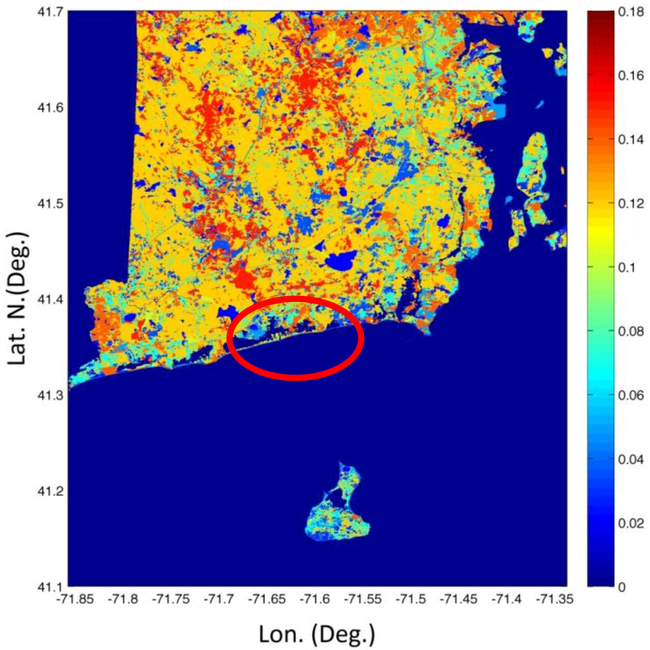
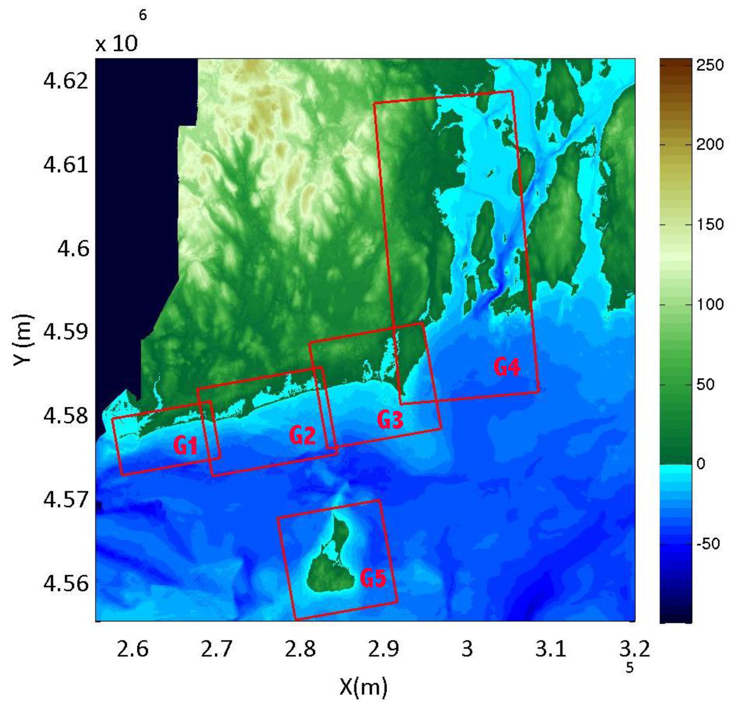
2.3. Digital Elevation Model (DEM)
3. Results and Discussion
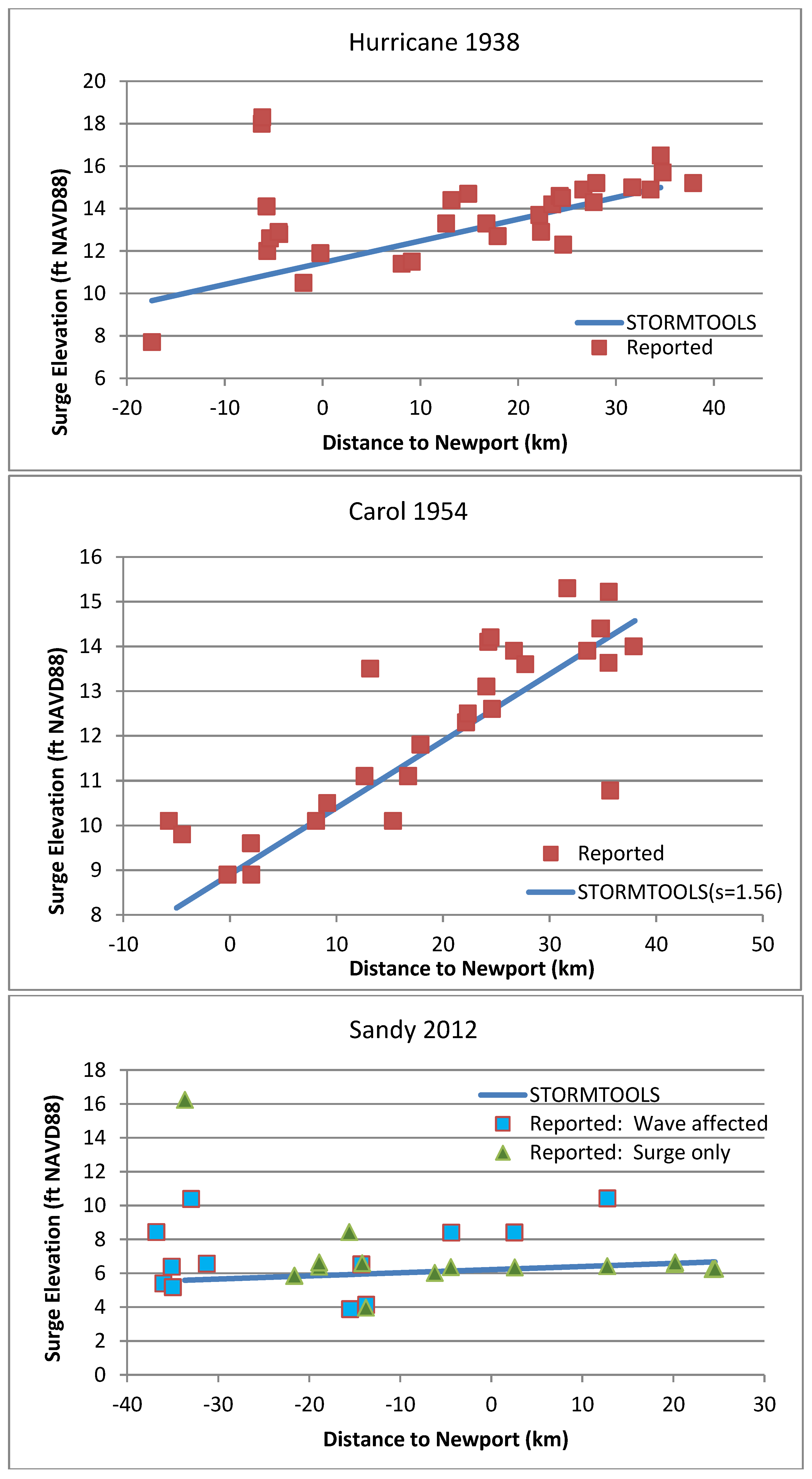
3.1. Surge and Tide Water Levels
3.2. Wave Modeling
3.3. Simulations
4. Conclusions
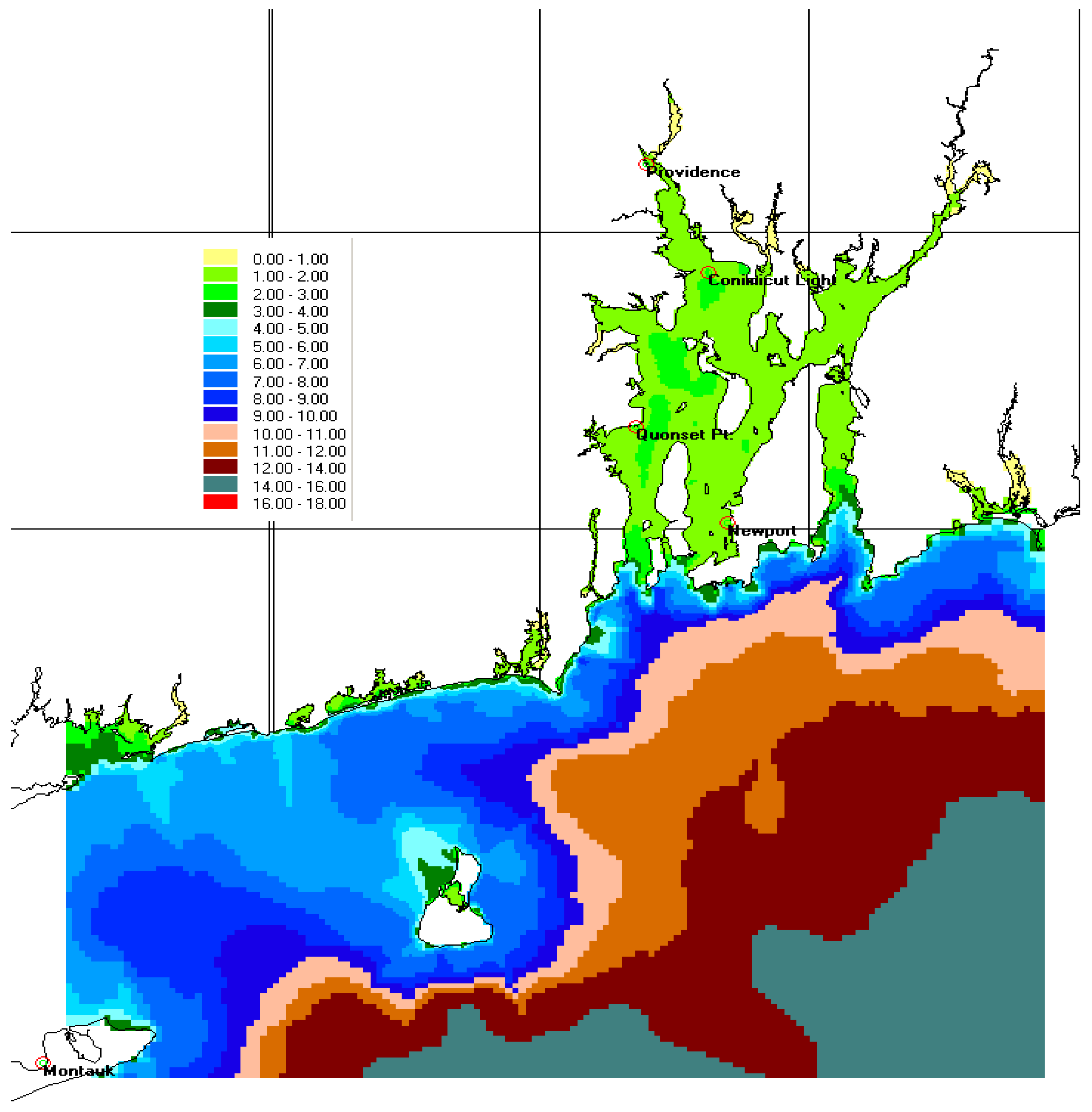
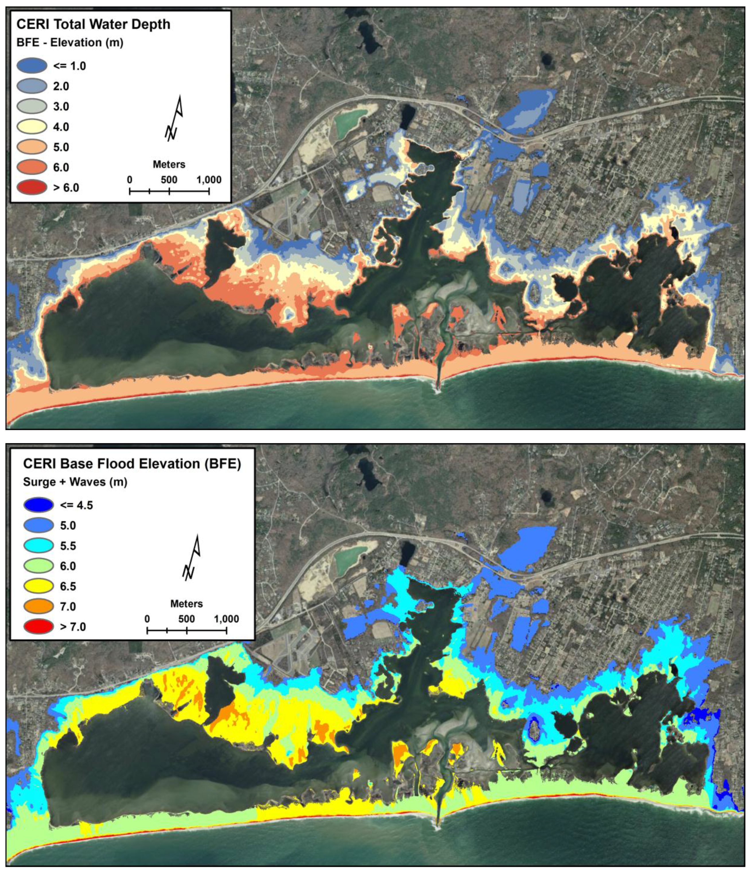
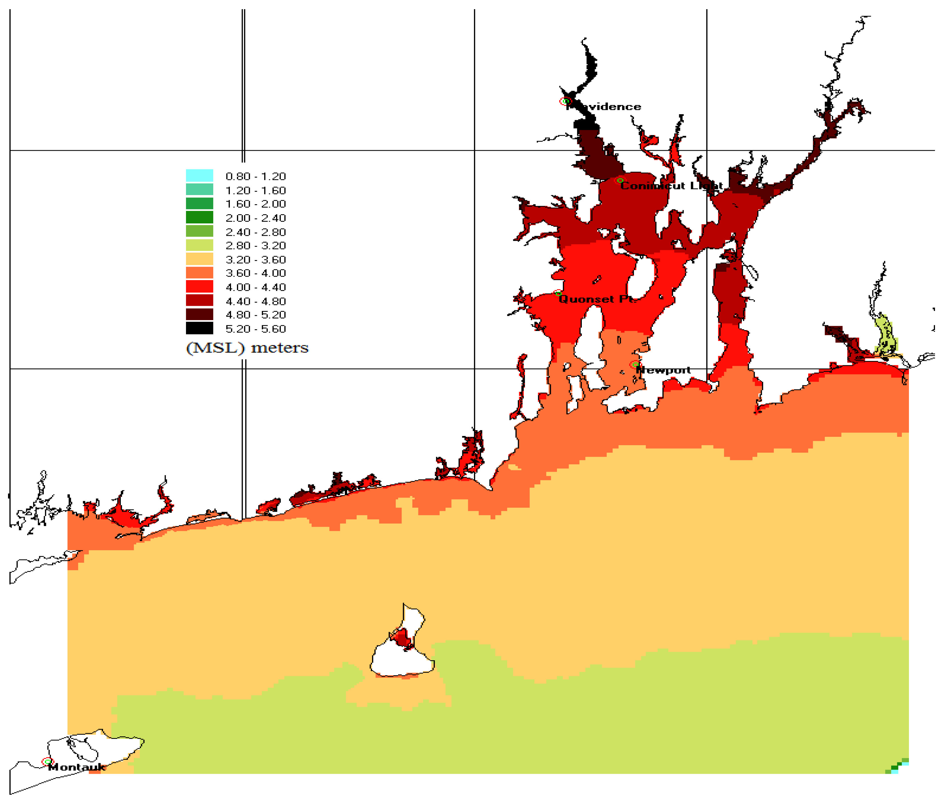
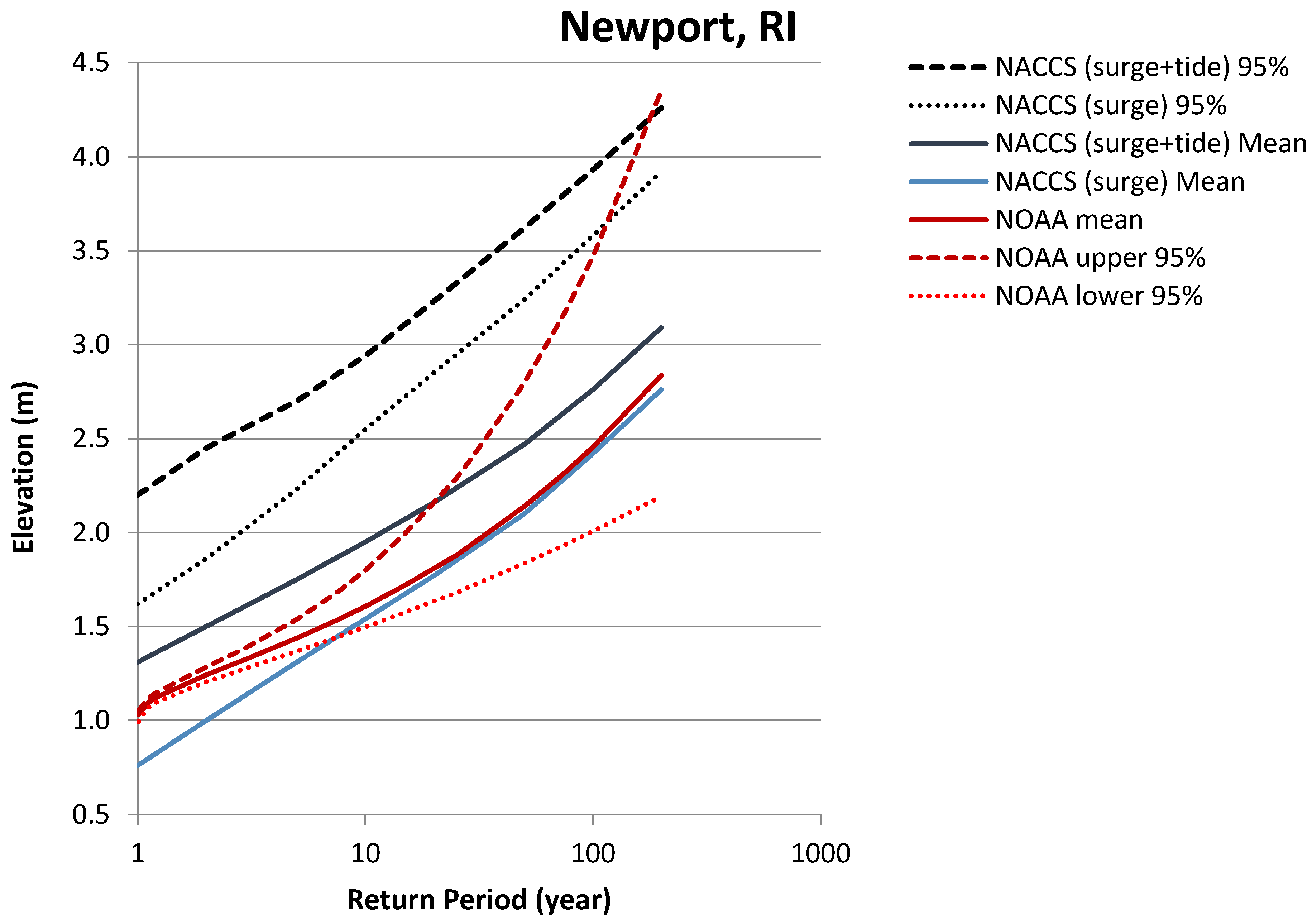
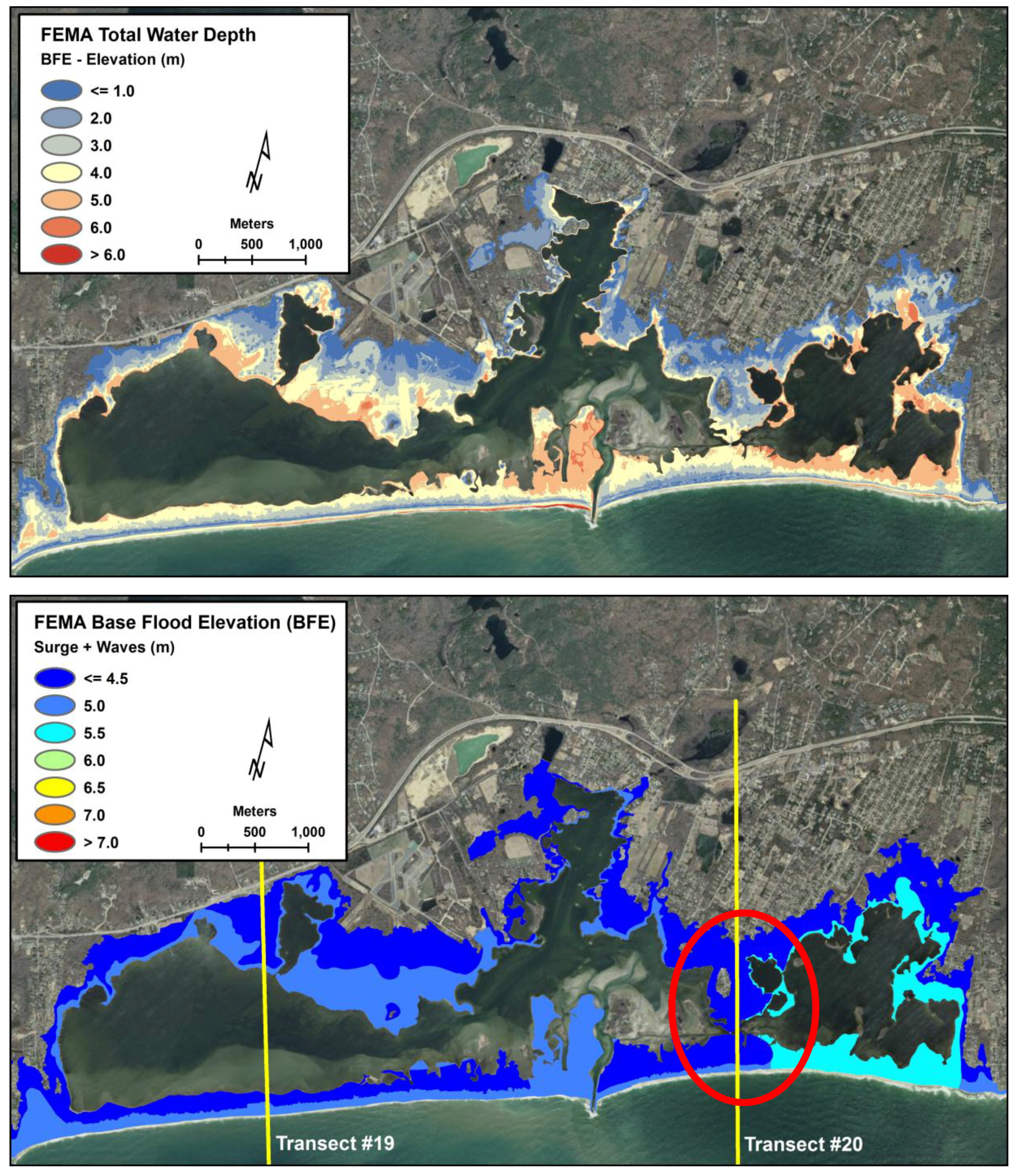
- FEMA and present study predict comparable SWEL for the study area. Present study values are slightly larger (4.1 m) than FEMA (3.7 m). This results in slightly larger inundated areas. The slightly larger values are attributed to the use of upper 95% confidence limit water levels used in the present study and the water level setup from the NAST simulations in the storm inundated area.
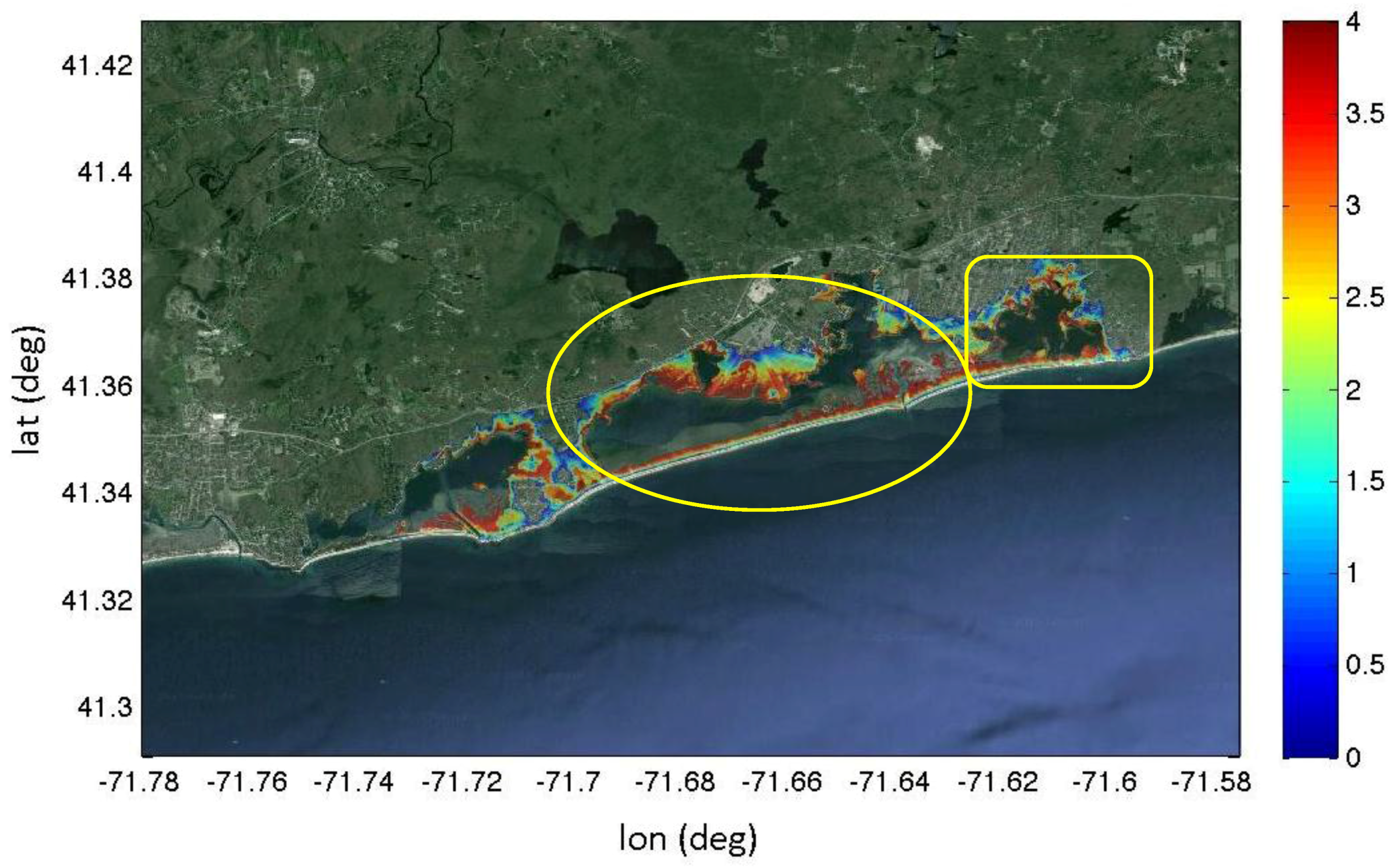
- The present study results show SWEL increasing with distance landward from the shoreline because of the balance between wind stress and frictional dissipation in flood inundated areas. FEMA’s SWELs are independent of distance landward.
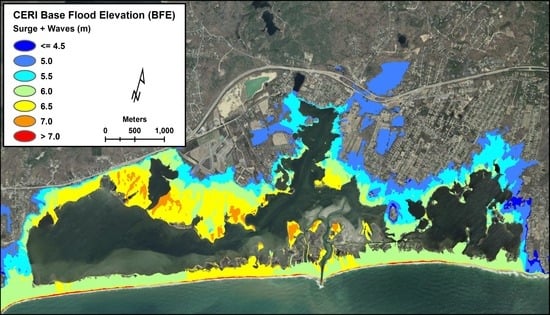
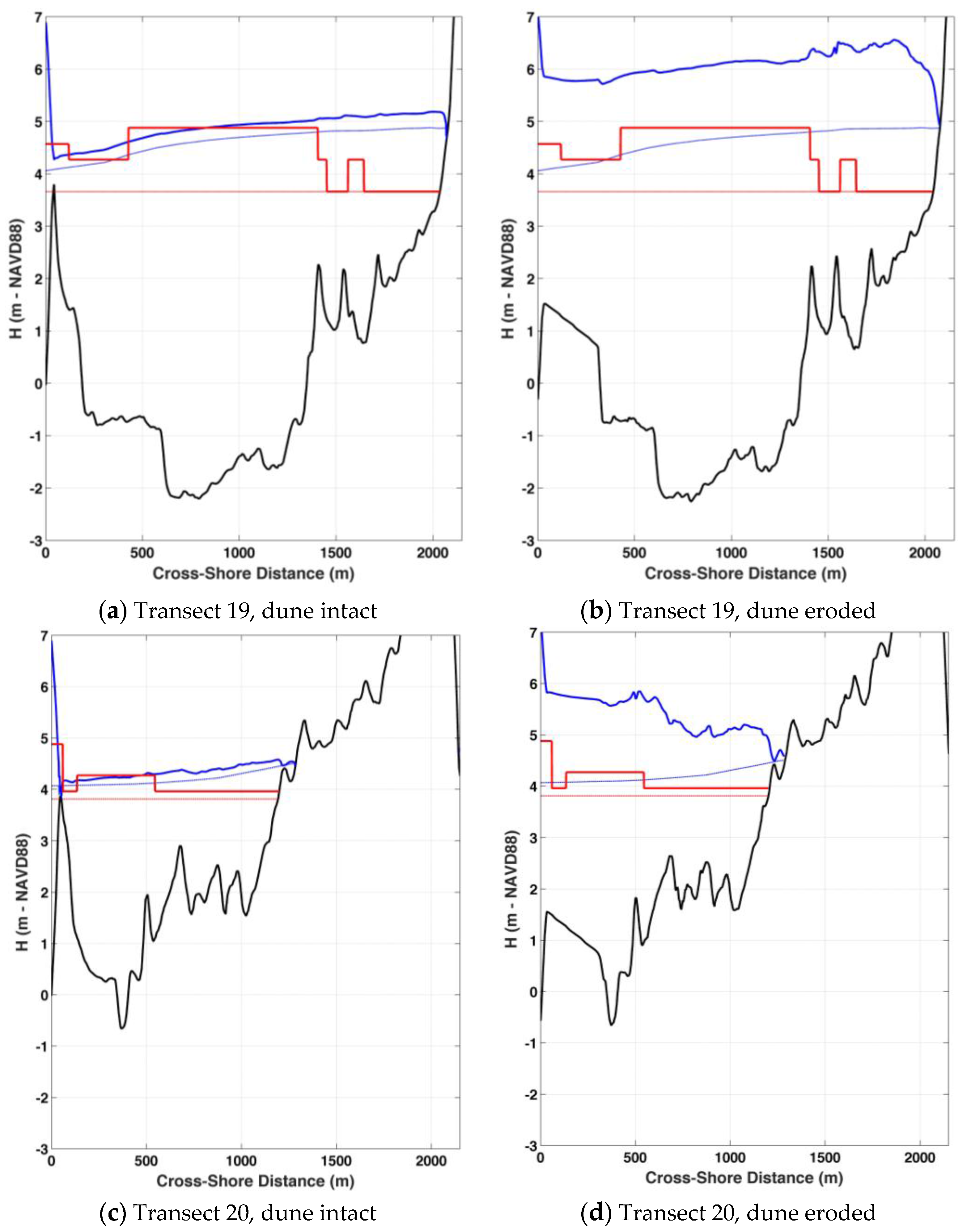
- FEMA (with eroded dunes) and the present study (with dunes assumed to be intact) predict comparable peak BFEs in the flood inundated areas. If the dunes are eroded FEMA results are substantially lower (about 1 m) than the present results. The primary source of differences is lower wave heights at the offshore end of the FEMA transects and differences in the eroded dune profiles. Attempts to obtain the FEMA bathymetry to use as input to WHAFIS for the two transects under study were not successful.
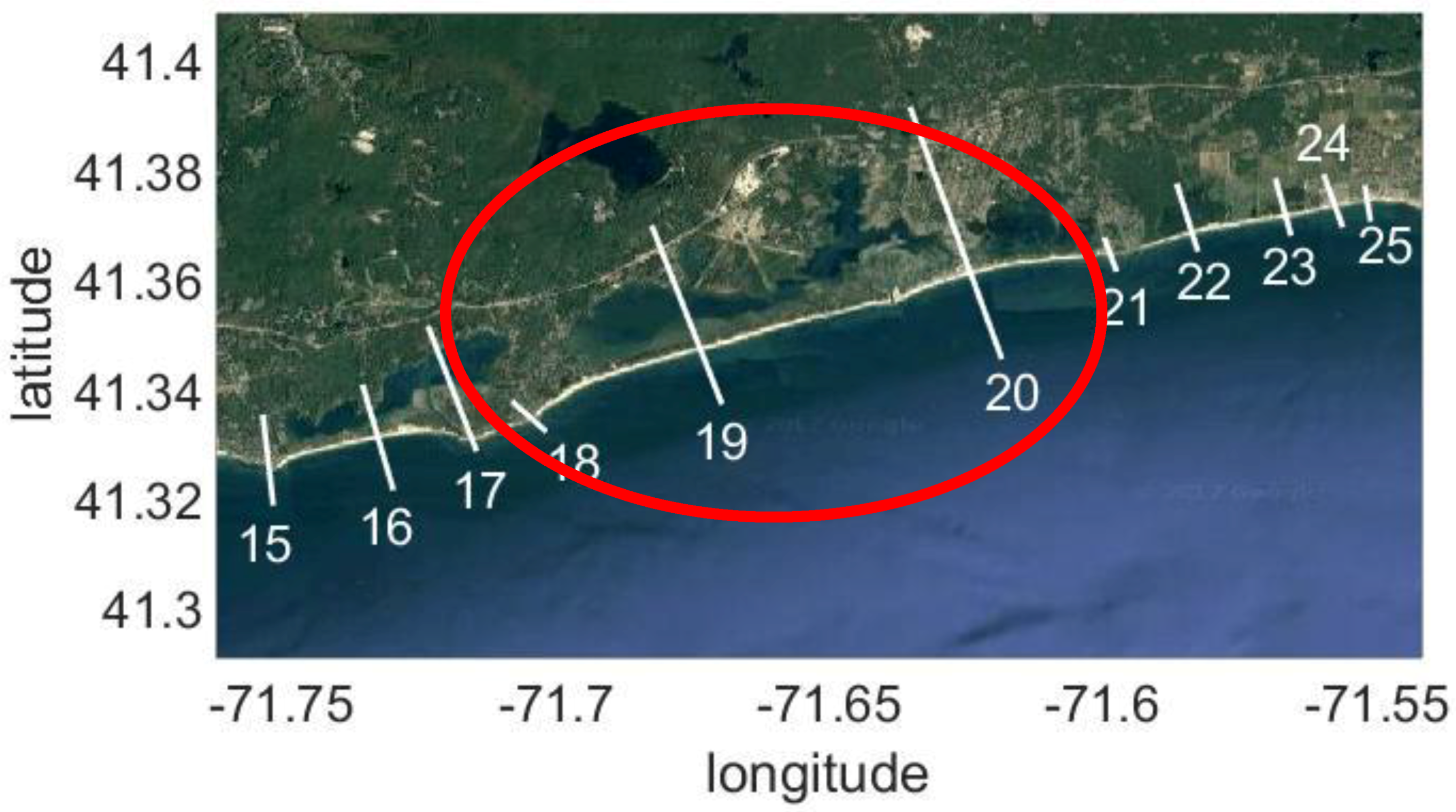
- FEMA results show strong evidence of the impact of the selection of the transects to represent wave conditions. As an example, for transect #20 the BFE shows a variation of almost 1.5 m from one side of the transect to the other at the dune crest line.
- It has proven impossible to recreate the 2-D structure of the wave field that FEMA has developed given the results for the two transects. It seems to be primarily controlled by topography. The transect spacing is too large to determine the spatial structure, and 2-D wave processes are not represented by the methods used (e.g., WHAFIS).
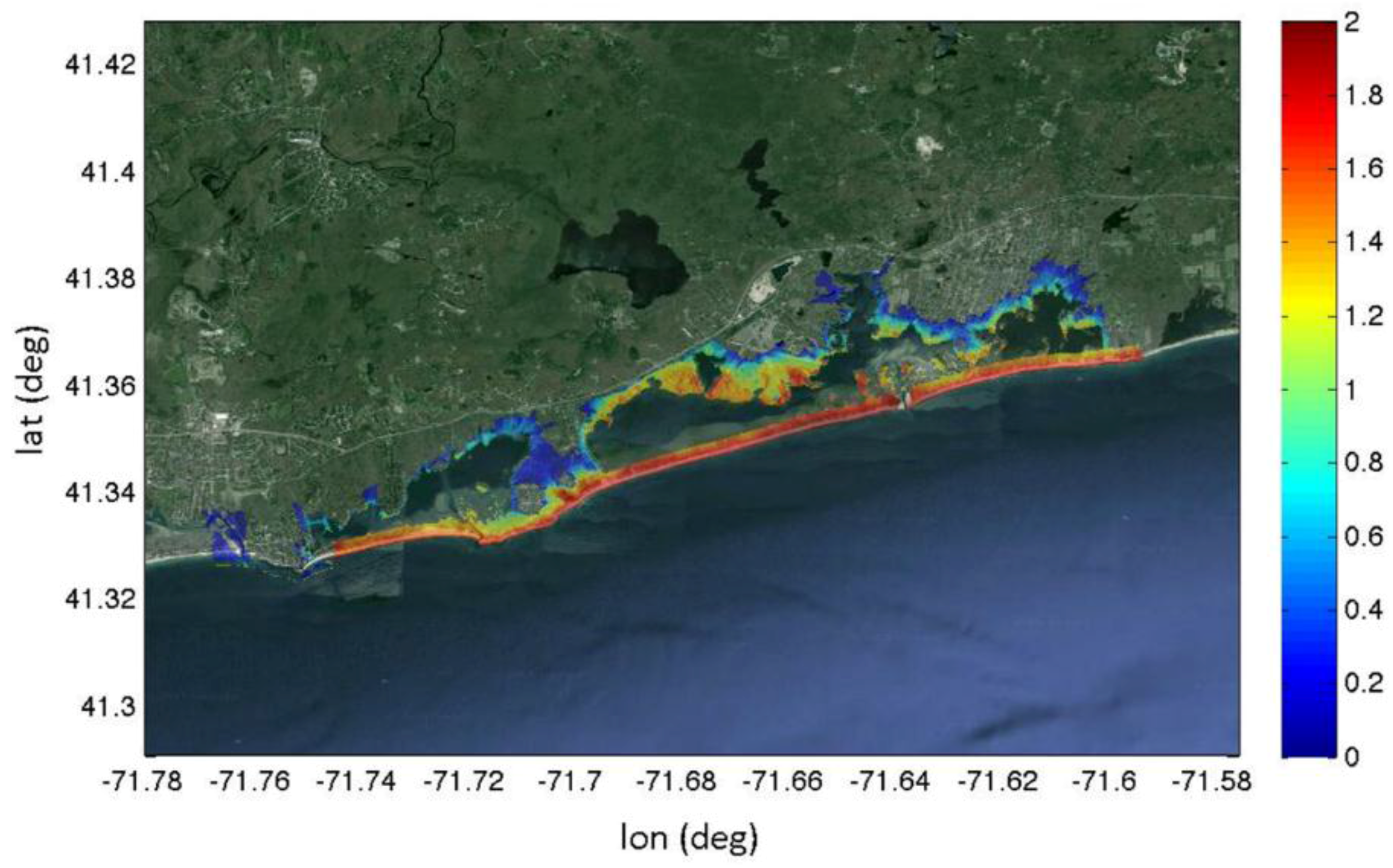
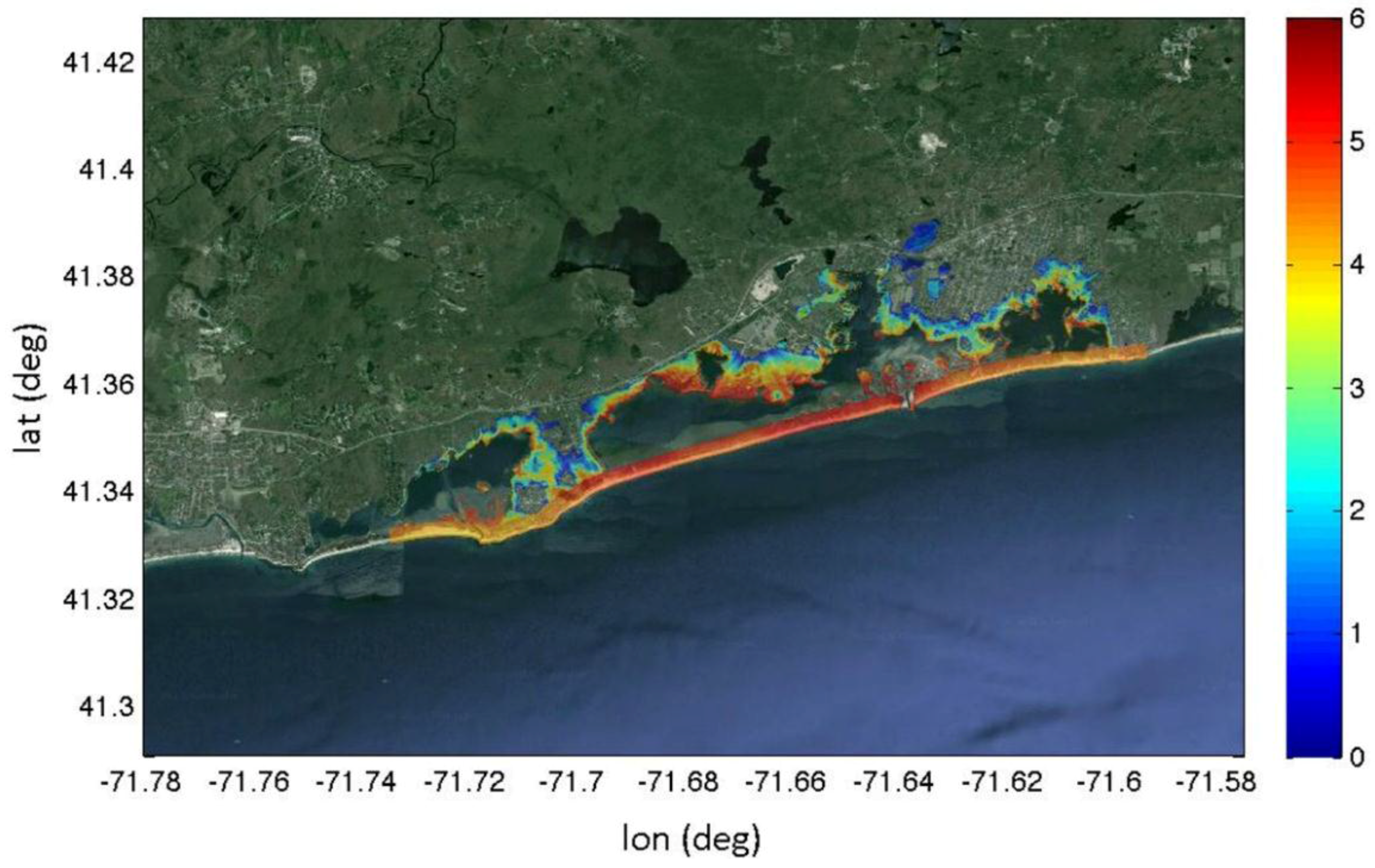
- The largest difference in the BFEs between the FEMA and present study methods is in the waves, particularly wave conditions at the shoreline and their subsequent 2-D spatial transformation. The present study predicts wave heights that are approximately twice as large as FEMA values. It has been impossible to determine which wave processes are critical in controlling the 2-D wave environment, but the initial indications are that they are caused by wave breaking along the eroded dunes, the specification of the eroded dune profile, and wave refraction and shallow water wave breaking on the landward edge of the coastal ponds and the nearby flood inundated areas.
Acknowledgments
Author Contributions
Conflicts of Interest
Acronyms
| ADCIRC | ADvanced CIRCulation model |
| ANN | Artificial Neural Network |
| BCP | Blind Control Points |
| BFE | Base Flood Elevation |
| CHAMP | Coastal Hazard Analysis and Modeling Program |
| CERI | Coastal Environmental Risk Index |
| CI | Confidence Interval |
| CRMC | RI Coastal Resources Management Council |
| DEM | Digital Elevation Model |
| FEMA | Federal Emergency Management Agency |
| FIRM | Flood Insurance Rate Maps |
| FIS | Flood Insurance Study |
| HUD | Housing and Urban Development |
| LAG | Lowest Adjacent Grade |
| LIDAR | Laser Imaging, Detection, and Ranging |
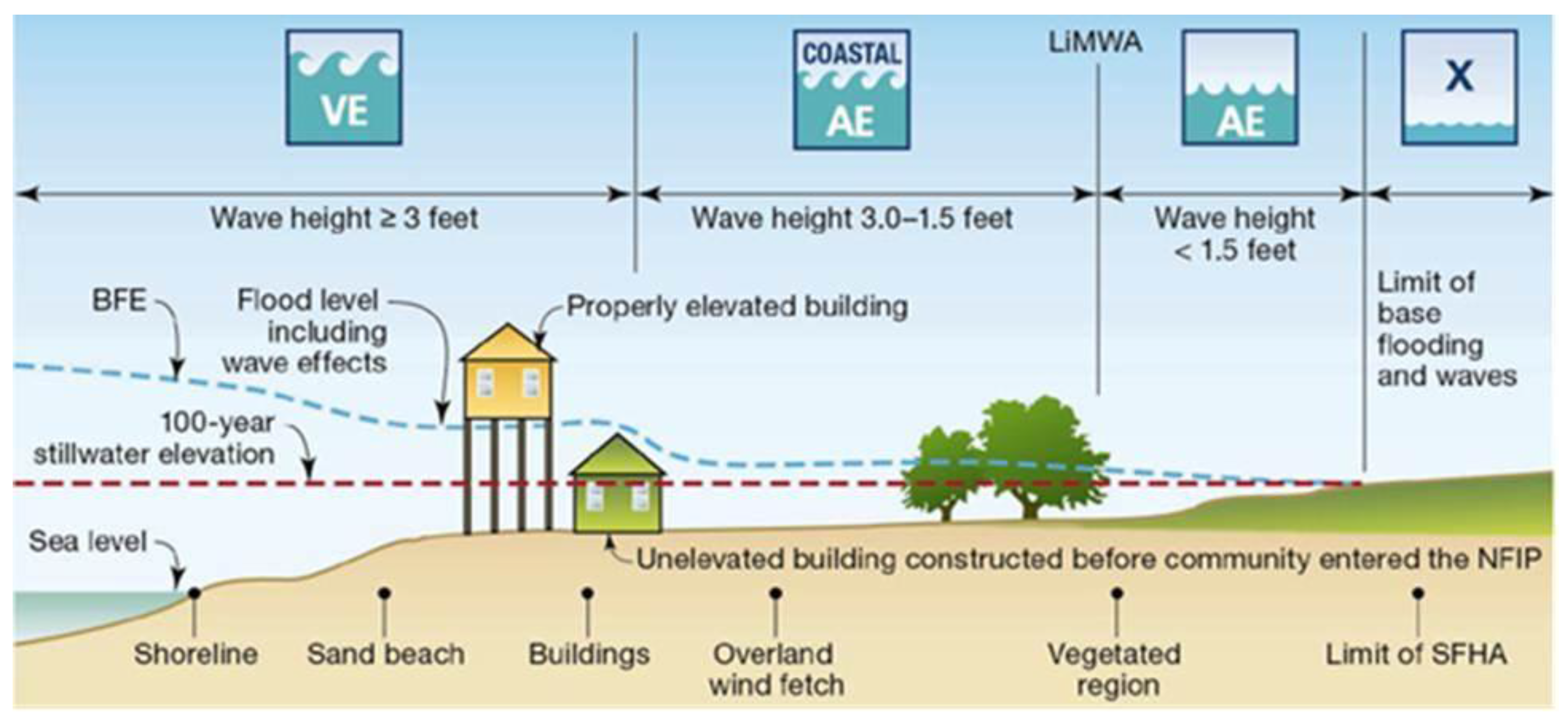
| LiMWA | Limit of Moderate Wave Action |
| MSL | Mean Sea Level |
| NACCS | ACOE, North Atlantic Coast Comprehensive Study |
| NAST | North Atlantic Coast Comprehensive Study and STWAVE |
| NAVD88 | North Atlantic Vertical Datum, 1988 |
| NOAA NOS | National Oceanic and Atmospheric Administration- National Ocean Survey |
| OHCD | Office of Housing and Community Development |
| RI GIS | Rhode Island- Geographic Information System |
| RMSE | Root Mean Square Error |
| SAMP | Special Area Management Plan |
| SLR | Sea Level Rise |
| STWAVE | STeady state spectral WAVE model |
| STORMTOOLS | tools in support of storm analysis |
| SWEL | Still Water Elevation |
| TMA | Texel, Marsen, and Arsloe wave spectrum |
| URI | University of Rhode Island |
| USACE | US Army Corp of Engineers |
| WAM | Wavewatch III, Model |
| WHAFIS | Wave Height Analysis for Flood Insurance Studies |
| WIS | ACOE Wave Information Study |
Appendix A

| Land Use | Manning |
|---|---|
| Open water | 0.02 |
| Low intensity residential | 0.07 |
| High intensity residential | 0.14 |
| Commercial industrial transportation | 0.05 |
| Bare rock/sand/clay | 0.04 |
| Quarries/strip mines/gravel pit | 0.04 |
| Transitional (cleared forest) | 0.1 |
| Deciduous forest | 0.12 |
| Evergreen forest | 0.15 |
| Mixed forest | 0.12 |
| Shrubland | 0.05 |
| Grassland/herbaceous | 0.034 |
| Pasture/hay | 0.03 |
| Row/crops | 0.035 |
| Small grain | 0.035 |
| Fallow | 0.03 |
| Urban recreational grasses | 0.025 |
| Woody wetlands | 0.1 |
| Emergent herbaceous wetland | 0.04 |

References
- Federal Emergency Management Agency (FEMA). Atlantic Ocean and Gulf of Mexico Coastal Guidelines Update (FEMA, 2007) to Appendix D, Guidance for Coastal Flooding Analyses and Mapping (FEMA, 2003); FEMA: Washington, DC, USA, 2007.
- FEMA. Flood Insurance Study, Washington County, RI, FEMA Flood Insurance Study Number 44009CV001B; FEMA: Washington, DC, USA, 2012.
- FEMA. Updated Tidal Profiles for the New England Coastline; Technical Report; FEMA: Washington, DC, USA, 2012. Available online: https://www.fema.gov/media-library/assets/documents/85240 (accessed on 16 January 2017).
- FEMA. WHAFIS Documentation Version 4.0. Available online: https://www.fema.gov/wave-height-analysis-flood-insurance-studies-version-40 (accessed on 16 January 2017).
- National Research Council (NRC). Mapping the Zone: Improving Flood Map Accuracy; Committee on FEMA Flood Maps; Board on Earth Sciences and Resources/Mapping Science Committee; The National Academies Press: Washington, DC, USA, 2009. [Google Scholar]
- FEMA Flood Zone Definitions. Available online: https://www.fema.gov/sites/default/files/images/flood_zones_limwa.jpg (accessed on 16 January 2017).
- FEMA Approved Numerical Models. Available online: https://www.fema.gov/coastal-numerical-models-meeting-minimum-requirement-national-flood-insurance-program (accessed on 16 January 2017).
- Cialone, M.A.; Massey, T.C.; Anderson, M.E.; Grzegorzewski, A.S.; Jensen, R.E.; Cialone, A.; Mark, D.J.; Pevey, K.C.; Gunkel, B.L.; McAlpin, T.O.; et al. North Atlantic Coast Comprehensive Study (NACCS) Coastal Storm Model Simulations: Waves and Water Levels (ERDC/CHL TR-15-44); Technical Report; Coastal and Hydraulics Laboratory U.S. Army Engineer Research and Development Center: Vicksburg, MS, USA, 2015. [Google Scholar]
- Spaulding, M.L.; Isaji, T.; Damon, C.; Fugate, G. Application of STORMTOOLS’s simplified flood inundation model, with and without sea level rise, to RI coastal waters. In Proceedings of the ASCE Solutions to Coastal Disasters Conference, Boston, MA, USA, 9–11 September 2015.
- Screening Tool for Assessing a Marina’s Environmental, Infrastructure, and Operational Risk to Storms and Flooding. Available online: http://www.beachsamp.org/resources/stormtools/ (accessed on 16 January 2017).
- Massey, T.C.; Anderson, M.E.; McKee-Smith, J.; Gomez, J.; Rusty, J. STWAVE: Steady State Spectral Wave Model. In User’s Manual for STWAVE, Version 6.0; US Army Corp of Engineers, Environmental Research and Development Center: Vicksburg, MS, USA, 2011. [Google Scholar]
- Smith, J.M.; Sherlock, A.R.; Resio, D.T. STWAVE: Steady-State Wave Model User’s Manual for STWAVE, Version 3.0; ERDC/CHL SR-01–01; Army Engineering Research and Development Center: Vicksburg, MS, USA, 2001. [Google Scholar]
- Oakley, B.A. Generalized 1% Storm Barrier Profile for the East Beach and Quonochontaug Barriers, Rhode Island; Technical Report Prepared for the Shoreline Change Special Area Management Plan; Coastal Resources Center, University of Rohde Island: Narragansett, RI, USA, 2016. [Google Scholar]
- Arcement, G.J.; Schneider, V.R. Guide for Selecting Manning’s Roughness Coefficients for Natural Channels and Flood Plains; U.S. Geological Survey Water-Supply Paper 2339; U.S. Geological Survey: Denver, CO, USA, 1989.
- Wamsley, T.V.; Cialone, M.A.; Smith, J.M.; Ebersole, B.A.; Grzegorzewski, A.S. Influence of landscape restoration and degradation on storm surge and waves in southern Louisiana. Nat. Hazards 2009, 51, 207–224. [Google Scholar] [CrossRef]
- RI Geographic Information System, Digital Elevation Models (DEM). Available online: http://www.rigis.org/data/topo/2011 (accessed on 16 January 2017).
- Sallenger, A.H., Jr. Storm impact scale for barrier islands. J. Coast. Res. 2000, 16, 890–895. [Google Scholar]
- Zervas, C. Extreme Water Levels of the United States, 1893–2010; Technical Report; NOAA: Silver Spring, MD, USA, 2013.
- Hashemi, R.; Spaulding, M.L.; Shaw, A.; Farhadi, H.; Lewis, M. An efficient artificial intelligence model for prediction of tropical storm surge. J. Nat. Hazards 2016. [Google Scholar] [CrossRef]
- Spaulding, M.L.; Grilli, A.; Damon, C.; Crean, T.; Fugate, G.; Oakley, B.A.; Stempel, P. STORMTOOLS—Coastal Environmental Risk Index (CERI). J. Mar. Sci. Eng. 2016, 4, 54. [Google Scholar] [CrossRef]
- USACE Wave Information System (WIS). Available online: http://wis.usace.army.mil/hindcasts.shtml?dmn=atlWIS (accessed on 16 January 2017).
- McArthur, B.; Coulton, K.; Dean, R.; Hatheway, D.; Honeycutt, M.; Johnson, J.; Jones, C.; Komar, P.; Lu, C.; Noble, R.; et al. Event-Based Erosion: FEMA Coastal Flood Hazard Analysis and Mapping Guidelines Focused Study Report; Technical report; FEMA: Washington, DC, USA, 2005.
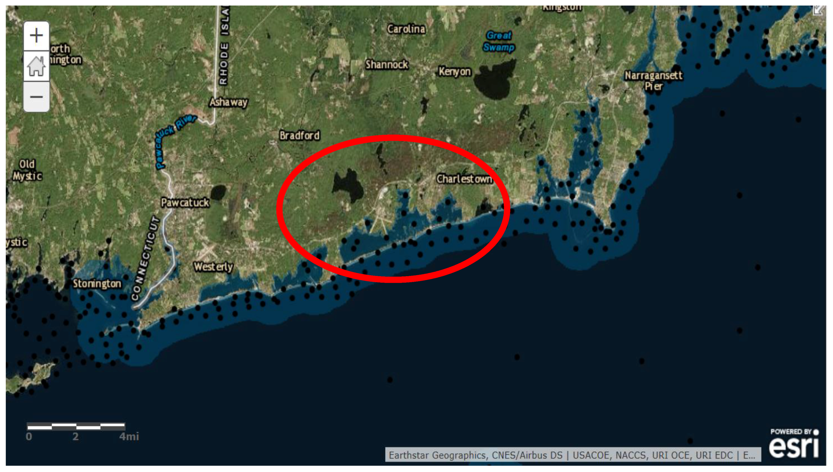
- FEMA. Flood Insurance Study for the Town of Charlestown, Rhode Island (Washington County); Community number 445395; FEMA: Washington, DC, USA, 1986.
- Jelesnianski, C.P. Bottom stress time-history in linearized equations of motion for storm surges. Mon. Weather Rev. 1970, 98, 462–478. [Google Scholar] [CrossRef]
- Dean, R.G.; Dalrymple, R.A. Coastal Processes with Engineering Applications; Cambridge University Press: Cambridge, UK, 2004. [Google Scholar]
- Spaulding, M.L.; Grilli, A.; Isaji, T.; Damon, C.; Hashemi, R.; Schambach, L.; Shaw, A. Development of Flood Inundation and Wave Maps for the Washington County, RI Using High Resolution, Fully Coupled Surge and Wave (ADCIRC and STWAVE) Models; Technical report; RI Coastal Resources Management Council: South Kingstown, RI, USA, 2015.
- USGS Water Level Data Sandy 2012. Available online: http://ga.water.usgs.gov/flood/hurricane/sandy/sites/hwm/HWM-RI-BRI-640.html (accessed on 18 January 2017).


| 100 Years Return Period Based on Generalized Extreme Value [GEV] at WIS 79 | ||||||
|---|---|---|---|---|---|---|
| Variable | WIS Time Series | NACCS Synthetic Storms | ||||
| 100 Year Mean | Lower 95% CI | Upper 95% CI | 100 Year Mean | Lower 95% CI | Upper 95% CI | |
| Hs (m) | 10.1 | 5.8 | 14.5 | 13.0 | 11.5 | 15.1 |
| Ws (m/s) | 32.8 | 24.5 | 41.0 | 39.3 | 33.9 | 47.9 |
| Tp (s) | 17.0 | 10.8 | 23.1 | 19.9 | 19.0 | 21.0 |
| Transect | Shoreline Coordinates (deg) | Water Elevation NAVD88 (m) | Critical Wave Crest (m) | Deep Water Significant Wave Height (m) [Hs] | ||||||
|---|---|---|---|---|---|---|---|---|---|---|
| FEMA | NAST | FEMA | NAST | FEMA | NAST | |||||
| Lat. N | Lon. W | SWEL + SETUP | BFE | SWEL + SETUP | BFE | |||||
| 19 | 41.338 | 71.670 | 3.7 | 4.6 | 4.1 | 6.9 | 0.9 | 2.8 | 4.0 | 7.0 |
| 20 | 41.346 | 71.619 | 3.8 | 4.9 | 4.1 | 7.0 | 1.1 | 2.9 | 4.0 | 7.0 |
© 2017 by the authors; licensee MDPI, Basel, Switzerland. This article is an open access article distributed under the terms and conditions of the Creative Commons Attribution (CC BY) license ( http://creativecommons.org/licenses/by/4.0/).
Share and Cite
Spaulding, M.L.; Grilli, A.; Damon, C.; Fugate, G.; Oakley, B.A.; Isaji, T.; Schambach, L. Application of State of Art Modeling Techniques to Predict Flooding and Waves for an Exposed Coastal Area. J. Mar. Sci. Eng. 2017, 5, 10. https://doi.org/10.3390/jmse5010010
Spaulding ML, Grilli A, Damon C, Fugate G, Oakley BA, Isaji T, Schambach L. Application of State of Art Modeling Techniques to Predict Flooding and Waves for an Exposed Coastal Area. Journal of Marine Science and Engineering. 2017; 5(1):10. https://doi.org/10.3390/jmse5010010
Chicago/Turabian StyleSpaulding, Malcolm L., Annette Grilli, Chris Damon, Grover Fugate, Bryan A. Oakley, Tatsu Isaji, and Lauren Schambach. 2017. "Application of State of Art Modeling Techniques to Predict Flooding and Waves for an Exposed Coastal Area" Journal of Marine Science and Engineering 5, no. 1: 10. https://doi.org/10.3390/jmse5010010