HTCRL: A Range-Free Location Algorithm Based on Homothetic Triangle Cyclic Refinement in Wireless Sensor Networks

1
College of Computer Science and Technology, Jilin University, Changchun 130012,
2
Computer Science and Information Technology Department, Daqing Normal University, Daqing 163712,
*
Author to whom correspondence should be addressed.
Information 2017, 8(2), 40; https://doi.org/10.3390/info8020040
Submission received: 3 January 2017
/
Revised: 8 March 2017
/
Accepted: 23 March 2017
/
Published: 27 March 2017
(This article belongs to the Special Issue Sensor Networks for Emergent Technologies)
Abstract
:Wireless sensor networks (WSN) have become a significant technology in recent years. They can be widely used in many applications. WSNs consist of a large number of sensor nodes and each of them is energy-constrained and low-power dissipation. Most of the sensor nodes are tiny sensors with small memories and do not acquire their own locations. This means determining the locations of the unknown sensor nodes is one of the key issues in WSN. In this paper, an improved APIT algorithm HTCRL (Homothetic Triangle Cyclic Refinement Location) is proposed, which is based on the principle of the homothetic triangle. It adopts perpendicular median surface cutting to narrow down target area in order to decrease the average localization error rate. It reduces the probability of misjudgment by adding the conditions of judgment. It can get a relatively high accuracy compared with the typical APIT algorithm without any additional hardware equipment or increasing the communication overhead.
1. Introduction
With the increasing development of wireless communication technologies, electronic technologies, embedded technologies, computer technologies and sensor technologies, the research and application of WSN (wireless sensor networks) is extensively popular and is a widespread concern. In recent years, wireless sensor have been widely used in the military field, intelligent agriculture, environmental monitoring, intelligent home system, and intelligent transportation system, search, rescue [1,2], etc. WSN consists of a large number of micro sensor nodes and each of them is energy-constrained and low-power dissipation. WSN is a kind of multi-hop and self-organizing network system. The sensors in wireless sensor network are distributed randomly in a designated area. In general, most of the sensor nodes are tiny sensors with small memories and do not acquire their own locations. This means determining the physical locations of the unknown sensor nodes is one of the key issues in WSN. The sensor node location information, however, is of great importance in many WSN applications. The location information could be used in geographical routing; reporting the location of an event; network management; target tracking; etc. [3,4].
In small-scale WSN, we could place the sensor nodes regularly and get the location of each node in advance. However, in practical applications, large numbers of sensor nodes always distributed randomly in large areas. Therefore, most sensor nodes’ locations cannot be known in advance. Since manual configuration of sensor nodes is not feasible for large-scale networks with mobile nodes, a possible way to localize sensor nodes is to use the global positioning system (GPS). GPS offers three-dimensional localization based upon direct line of sight with at least four satellites [5]. However, using GPS to location for all the unknown nodes is not feasible. The reasons are as follows. (i) It is unavailable in indoor environments; (ii) the GPS is an energy-consumption module which reduces the lifetime of the sensor networks; (iii) GPS is also a relative large and expensive module which would not reduce the cost of the large scale sensor networks. Therefore, how to locate the location of the unknown node in sensor networks by a feature of the network itself is a significant topic which is of great concern to researchers and manufacturers.
Specifically, there are two kinds of nodes in sensor networks. The first is anchor nodes which could determine their own location with hardware equipment such as GPS, and the second is unknown nodes which could not locate themselves with hardware equipment. The purpose of localization algorithms is to locate the unknown nodes through, the features and knowledge of the sensor networks without hardware assistance.
Recently, a body of methods and algorithms has been proposed to find solutions for locating the unknown nodes in WSNs, including range-based algorithms and range-free algorithms. Range-based algorithms need node-to-node distances or angles for estimating the locations of unknown nodes. Range-based algorithms use the time of arrival (TOA) [6], Time Difference of Arrival (TDOA) [7], Angle of Arrival (AOA) [8], Radio Interferometry Positioning System (RIPS) [9] and Received Signal Strength Indication (RSSI) [10]. These algorithms have lower localization error rates than the range-free algorithms but require additional hardware to obtain the information on distances or angles. Meanwhile, range-free algorithms depend on connectivity information network knowledge, such as the DV-hop algorithm [11,12], Approximate Point-in-Triangulation test algorithm (APIT) [13], amorphous algorithm and centroid algorithm [14,15,16]. Therefore, the range-free localization algorithm is widely used in practical applications especially in large scale deployment environment since the lower cost and additional hardware-free features.
APIT is a range–free algorithm which is simple and easy to implement. It is low in communication cost and energy consumption. It also has a low location error rate. However, the performance of the APIT algorithm is largely affected by the density of anchor nodes and is restricted for the In-to-Out Error and Out-to-In Error, so there exists space to improve this algorithm.
In this paper, an improved APIT algorithm HTCRL (Homothetic Triangle Cyclic Refinement Location) is proposed, which is based on the principle of the homothetic triangle. It involves narrowing the triangle in proportion which contains the unknown node to improve the accuracy of node location. The improved APIT algorithm could get a relative low localization error rate compared with the typical APIT algorithm without any additional hardware or increasing the communication overhead.
2. Related Work
In this section, we introduce the APIT algorithm. It is a range-free location algorithm of unknown nodes.
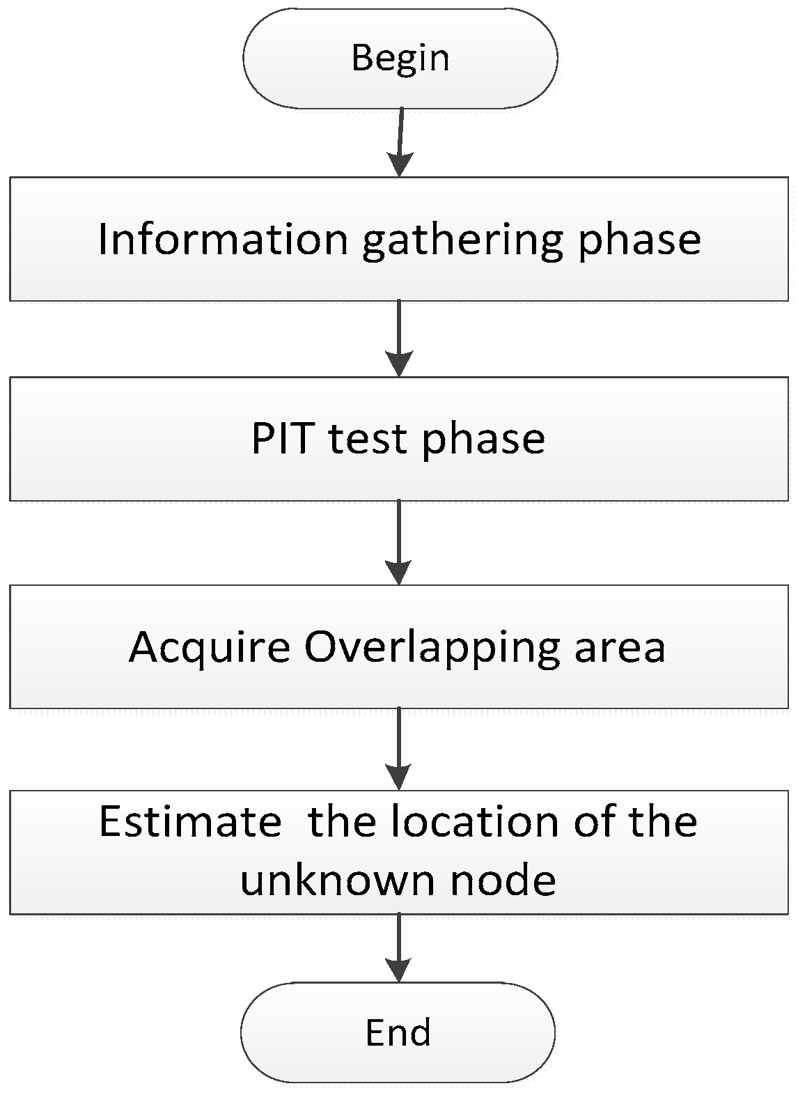
The APIT (approximate point in test) [17] algorithm is a range-free WSN localization algorithm. The main principle of APIT algorithm is utilizing the centroid of the overlap sections of the triangles formed by the connected anchors to estimate the location of the unknown nodes. Specifically, the principle is show in Figure 1. In Figure 1, assuming there are anchors connected to the unknown nodes (the black circle in Figure 1). The unknown node selects 3 nodes from all the connected anchors. Suppose the number of the connected anchors are . It has different triangles. Then, test whether the unknown node is in the triangles that they select. The process of the test is repeated until all of the ternary combination are exhausted or the desired localization error rate is reached. Then, it calculates the centroid coordinate of the coverage overlap area of all triangles as the coordinate of the unknown node. As shown in Figure 1, the centroid of the overlap polygon is the estimated coordinates of the unknown nodes. From Figure 1, the black spot is the unknown node coordinate [18,19]. The main phase of APIT is shown in Figure 2.
Step 1: Unknown nodes gathering the information on the anchor nodes.
In Step 1, all anchor nodes in the area broadcast their location information. The broadcasting message includes its position information and ID. The nodes (includes other anchor nodes and all unknown nodes) collects the messages and exchange the message (including the value of RSSI) with their neighbor unknown nodes [20]. The format of the message is shown in Figure 3.
The unknown nodes test whether they are inside the triangle composed of the three connected anchors. If the unknown node is inside the triangles the algorithm will calculate the centroid coordinator of all the triangles’ overlap area [21].
Step 2: PIT (Point-In-Triangulation Test) test stage.
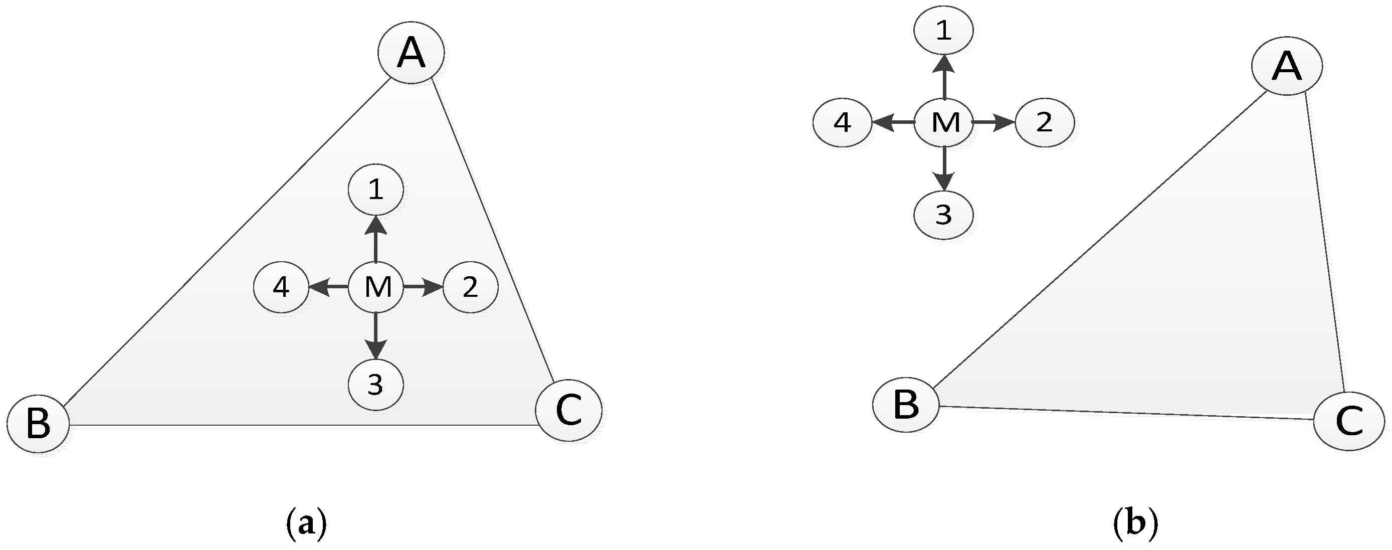
The key of the APIT is to judge whether the unknown nodes inside the triangle. In generally, the Perfect Point-In-Triangulation Test method is used to solve this problem in APIT. The principle of the PIT is shown in Figure 4. For any ΔABC and point N on the two dimensional plane, if such a direction exists the unknown node moves along; when the unknown node moves close to one of the anchor nodes A, B and C, it will be far away from the other two nodes, and we can deduce that the unknown node is inside the triangle. The principle is shown in Figure 4a. We also can deduce that if the unknown node is out of the triangle when the unknown node moves along a direction far away from the three anchor nodes A, B and C simultaneously. The principle is shown in Figure 4b.
However, the nodes are deployed randomly in WSN and most of them are static, so the nodes cannot move. One solution is with the help of the neighbor nodes. In Figure 5 it is the principle of APIT test. The SS (Signal Strength) received by the unknown node is inversely proportional to the distance from the anchor node. In Figure 5a, assuming that the node M moves to the node 1, 2, 3 and 4 then tests their SS. The unknown node M exchanges the message with its four neighboring nodes 1, 2, 3 and 4. For example, the unknown node M will compare the SS with node 1 and find that the SS of node M received from node A is lower than node 1. But the SS of node M received from nodes B and C is higher than node A. Thus, when node M moves to node 1, it will near node A but is far away from nodes B and C. This suggests the conclusion that node M is inside ΔABC. In the same way, it can judge nodes 2, 3 and 4. The conclusion is the same. In Figure 5b, when node M moves to node 4, it is far away from nodes A, B and C; therefore M thought it was outside ΔABC.
Step 3: Acquire triangles’ overlapping area.
From Step 2, the unknown node encompassed by several triangles then uses the grid scan algorithm to acquire the overlapping area. When the grid is inside any triangle the grids’ count (initialized by 0) in the triangle will be plus 1 in the corresponding area.
Step4: Grid scanning.
If the unknown node is in the triangle composed of three anchor nodes, then the grid count (initialized by 0) in the triangle will decrease by 1. The principle is shown in Figure 6.
From Step 3, we can find the max count of several grids, and then calculate the centroid of the polygon composed by the grids. The formulas are as shown in Formulas (1) and (2).
In Formulas (1) and (2), x presents the horizontal coordinate of the unknown node, y presents the vertical coordinate of the unknown node, and (xi, yi) presents the coordinates of the grids with the max count.
From the four steps above, the coordinates of the unknown node are known. But it cannot meet the extra low localization error rate requirements in some applications. Theoretically, APIT algorithm could be improved by calculate the fine-grained triangles overlap section to decrease the localization error rate. This paper depends on this theory, proposes an improved APIT algorithm, HTCRL algorithm, to optimize the localization error rate of APIT algorithm.
3. HTCRL Algorithm
3.1. Mathematical Model
In order further decrease the localization error rate, in this paper the homothetic triangle is used to narrow the triangle coverage area. The triangle narrows down gradually until it satisfies accuracy requirements.
As an improvement of the APIT localization algorithm, the HTCRL algorithm adopts the “Perpendicular Median Surface Cutting” to narrow down targeted area in order to decrease the localization error rate. It reduces the probability of misjudgment by adding the conditions of judgment.
Definition 1.
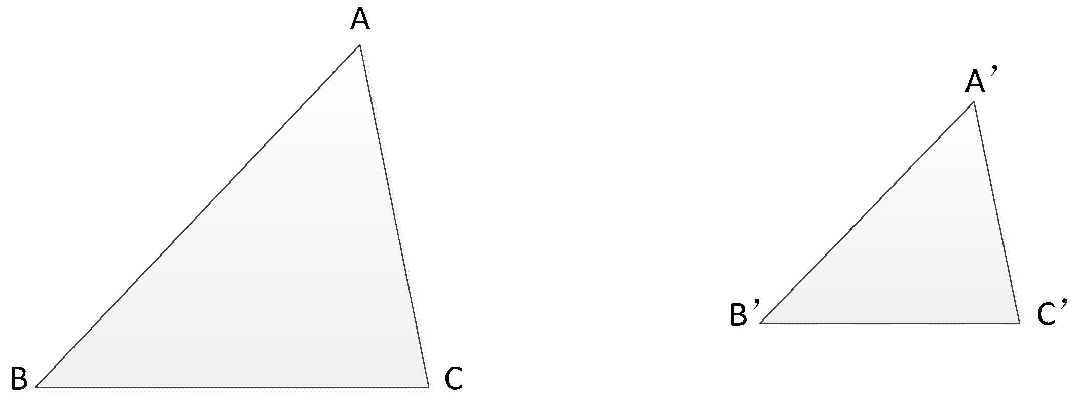
Homothetic triangle. Suppose that two triangles are homothetic if a pair of corresponding angles is equal and the corresponding edges are in proportion.
Definition 2.
The center of the triangle. The angular bisector of the three angles integrates into one point. The point is the center of a triangle’s inscribed circle, which is called the center of a triangle. (The distance between the point and the three sides of the triangle is equal.)
An example is shown in Figure 8. As is shown in Figure 8, O is the center of ΔABC, and OD, OE and OF are the heights of the three sides. Then α1 = α2, β1 = β2, γ1 = γ2, OD = OE = OF.
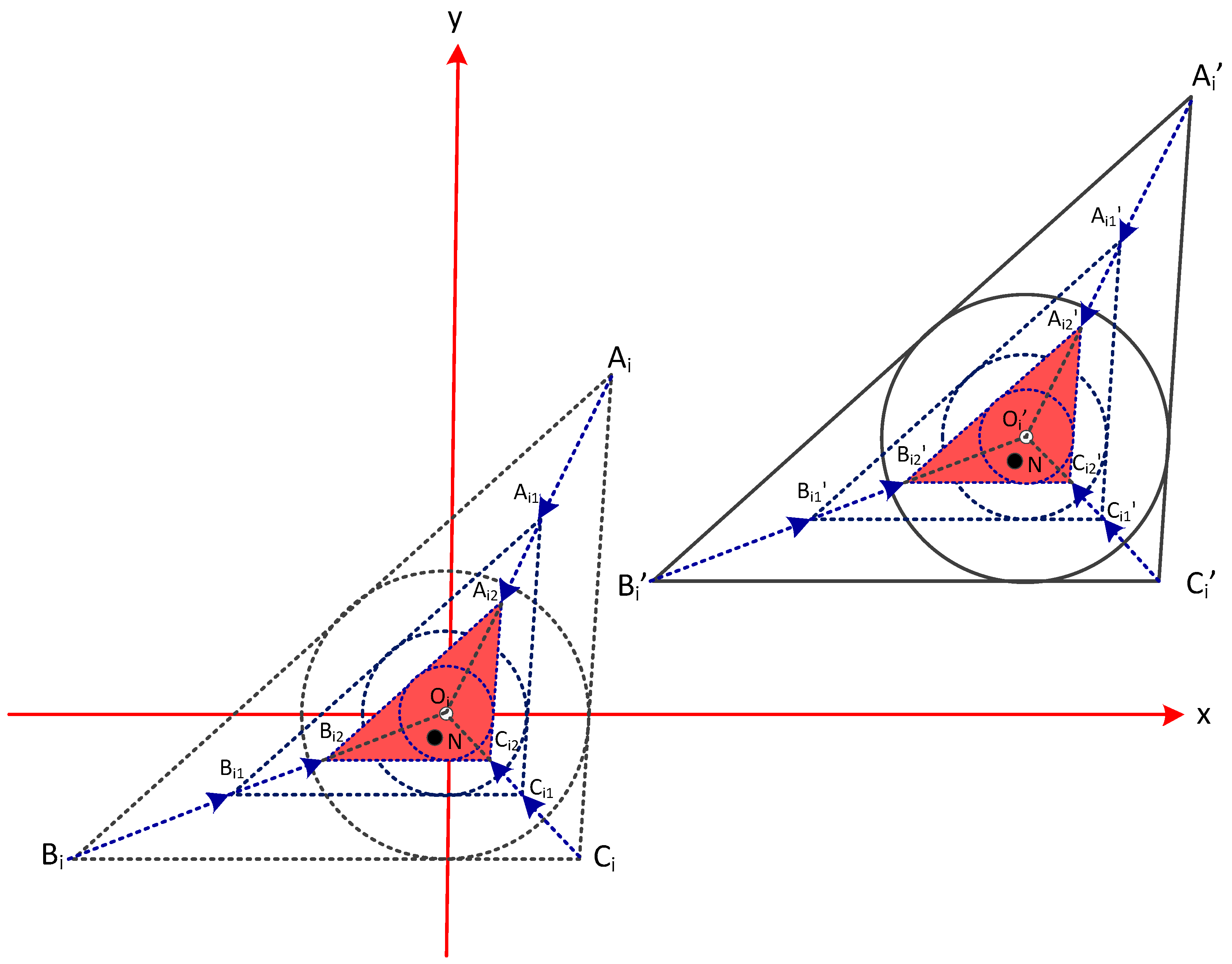
The improved APIT algorithm adopts the homothetic triangle to narrow down the targeted area. According to the theory of the homothetic triangle, the area of the triangle that encompassed the unknown node will be narrowed down gradually. The principle of the algorithm is shown in Figure 9.
As shown in Figure 8, the center of all the homothetic triangles is the origin coordinates of two-dimension which is denoted by . is the estimate coordinator of the unknown node N. In the beginning, through PIT test we will get several triangles which encompassed the unknown nodes N. In this stage the purpose is to narrow down the triangle area. is the ith (i = 1, 2, 3 … n) that encompasses unknown node N. can be narrowed down to , j = (1, 2, 3 …), the variable j represents the times that the triangle narrow. For example, in Figure 8, can be narrowed down to . can be narrowed down to . ∽ ∽ . The vertex of the triangle moves along the angular bisector simultaneously to narrow down the area. The coordinators of the three vertexes in are , and . is narrowed down in proportion that the proportion could be supposed k (i = 1, 2, 3 …), If the triangle has narrowed down j times, the coordinators of are .
In APIT the nodes Ai’, Bi’ and Ci ’are the anchor nodes and their coordinators are known in advance. The coordinators of Ai’, Bi’ and Ci’ are , and , therefore the coordinator of node Oi’ can be calculated through Formulas (3) and (4). The coordinator of node is .
In Formulas (3) and (4),
In order to calculate the centroid coordinates of the narrowed triangles, for simplicity of calculation it will translate the coordinate axis and the coordinate of will be . After translating the coordinate axis the coordinates of and will be and , and separately they are A. After narrowing down the translations and translating the coordinate axis, the coordinates are . The value of them are shown in Formula (8). Now three vertex of the translation are available. It can be used in node location algorithm. K is the proportion by which the triangles reduced.
3.2. The Main Algorithm Flow Descriptions of HTCRL
The improved range free location algorithm based on homothetic triangle cyclic refinement proposed in this paper can decrease the localization error rate efficiently. In APIT algorithm, the size of the overlapping triangle area which embraced by the anchor nodes has a great impact on algorithm performance. Localization accuracy will be greatly improved as the area is reduced gradually. For this, in this paper we proposed a localization algorithm to assist localization, the localization accuracy will be improved by this method.
The main process of HTCRL (Homothetic Triangle Cyclic Refinement Location) algorithm is shown in Figure 10.
Step 1: Initialize the network configuration.
Step 2: Each anchor node in the area broadcasts the messages including their own location information and ID. The nodes (includes other anchor nodes and all unknown nodes collect the messages (ID, position, RSS) and exchange the message with their neighbor unknown nodes.
Step 3: The unknown nodes judge whether they have received the message from more than three anchor nodes? If the number is more than three, it will go to Step 4. If the number is less than three, it will go to Step 7.
Step 4: PIT (Point-In-Triangulation Test) test stage. It will judge whether they are inside the triangle composed by the three neighbor anchors. If the unknown node is inside the triangles, HTCRL algorithm begins to narrow down these triangles until the localization error rate is satisfied for the applications.
Step 5: Acquire triangles overlapping area.
Step 6: Use the homothetic triangle cyclic refinement algorithm to calculate the centroid of the overlapping area in Step 5, which is the estimated coordinates of the unknown nodes.
Step 7: end.
4. Simulation and Result
4.1. The Parameters of Network in Experiments
In our experiments, several parameters are studied that affect the localization error rate directly in the HTCRL algorithm. The parameters of network include anchors heard, node density, anchor percentage, anchor to node range ratio. In this paper, suppose the radio model is perfectly circular.
Anchors Heard (AH): This parameter is defined as average number of anchors that a node heard and used in experiment. In the network, the more anchors heard the accuracy is better. However, the more anchors heard the cost is higher. In our experiments, the number of anchors nodes in the network is from 3 to 21.
Node Density (ND): This parameter is defined as average number of nodes in a hop communication range. The nodes include unknown nodes and anchor nodes.
Anchor Percentage (AP): This parameter is defined as the percentage of anchors in all sensor nodes. The values can be calculated in Formula (9). In the following, it uses as anchor percentage. That is the number of anchors divided by the number of anchors and the unknown nodes.
Anchor to Node Range Ratio (ANR): This parameter is defined as the average radio range of the anchor divides by the average radio range of the unknown node. From our past experiments, the value most suitable value is 3.
4.2. The Performance of the Localization Algorithm
Assume the actual coordinate of the unknown nodes is , The estimated coordinate of the unknown nodes is . n is the number of the unknown nodes; R is the radio range of the unknown nodes. In the experiment, the localization error is tested through , which is shown in Formula (10).
In order to verify the performance of HTCRL localization algorithm, the algorithm is simulated through MATLAB R2012a. In this section, several parameters which affect the performance of HTCRL localization algorithm are analyzed in our simulations. It is assumed that the experiments are done in a two dimensional 1000 m × 1000 m area. The sensor nodes are distributed randomly and uniformly in the area respectively.
Random distribution is when unknown nodes and anchors are distributed randomly. Uniform distribution is when the area is divided into several grids and the unknown nodes and anchors are distributed randomly in the grids. It can ensure the sensors are placed at equal distances.
The number of anchors can be adjusted according to the communication connectivity of the network. The experiments are repeated 300 times and the average value is used as the final result.
There are 1000 sensor nodes spread out in the area.
1. Localization Error Varying with Anchor Heard(AH) and Communication Radius (R)
In this experiment, we analyzed the parameters of anchor heard and communication radius (R) that influent localization error rate.
In Figure 11a, the parameters are as flows: AH = 3~21, ANR = 3, ND = 8, R = 150 m, K = 0.0050. The sensor nodes are distributed in random distribution. Figure 11a shows that the overall trend of localization error rate in APIT and HTCRL localization algorithms decreases as the number of anchors heard increases. Instead, HTCRL localization algorithms performs better than APIT. The localization error rate of APIT is from 38.2% to 23.1%, while the localization error rate of HTCRL is from 35.3% to 22.5%.
In Figure 11b, the parameters are as follows: AH = 3~21, ANR = 3, ND = 8, R = 150 m, K = 0.0050. The sensor nodes are distributed in uniform distribution. Figure 11b shows that the overall trend of localization error rate in APIT and HTCRL localization algorithms decreases as the number of anchors heard increases. Instead, HTCRL localization algorithms perform better than APIT. The localization error rate of APIT is from 32.2% to 19.0%, while the localization error rate of HTCRL is from 30.1% to 18.9%.
From Figure 11a,b, we note that HTCRL localization algorithm is more accurate than the APIT localization algorithm when they have the same parameters. In addition, comparing random distribution and uniform distribution, the performance in uniform distribution is better than in random distribution.
In Figure 11c, the parameters are as flows: AH = 3~21, ANR = 3, ND = 8, R = 450 m, K = 0.0050. The sensor nodes are distributed in random distribution. Figure 11c shows that the overall trend of localization error rate in APIT and HTCRL localization algorithms decreases as the number of anchors heard increases. Instead, HTCRL localization algorithms performs better than APIT. The localization error rate of APIT is from 60.1% to 31.2%, while the localization error rate of HTCRL is from 52.1% to 28.9%.
In Figure 11d, the parameters are as follows: AH = 3~21, ANR = 3, ND = 8, R = 450 m, K = 0.0050. The sensor nodes are distributed in random distribution. Figure 11d shows that the overall trend of localization error rate in APIT and HTCRL localization algorithms decreases as the number of anchors heard increases. Instead, HTCRL localization algorithms performs better than APIT. The localization error rate of APIT is from 48.2% to 30.1%. However, the localization error rate of HTCRL is from 45.1% to 26.9%.
From Figure 11c,d, we note that HTCRL localization algorithm is more accurate than APIT localization algorithm when they have the same parameters. In addition, by comparing random distribution and uniform distribution, the performance in uniform distribution is better than in random distribution.
In the above experiments, the communication radius (R) is 150 m and 450 m separately. It can be seen from Figure 11 that the localization error rate is higher when R is 450 m. Therefore, communication radius (R) is not greater when the localization error rate is lower in the two algorithms.
In the experiments, the localization error rate decreases when the number of anchors heard is from 3 to 21 and the communication radius is constant. When the value of AH increases gradually, it will increase the cost of the network. However, from the results of the experiments, when AH is from 3 to 9, the localization accuracy has been meet the requirements of outdoor localization. Therefore, it does not need to increase the value of AH gradually for little improvement in localization accuracy. Thus, the cost of the network will not increase a lot when it meet the requirements of outdoor localization.
2. Localization Error Varying Node Density (ND) and Anchor Percentage (AP)
This experiment analyses the parameters of node density (ND) and anchor percentage (AP) that influence localization error rate. In the experiment, the sensor nodes distributed in random distribution.
In Figure 12a, the parameters are as follows: AH = 18, ANR = 3, AP = 20%, R = 150 m, K = 0.0050. The sensor nodes are distributed in random distribution. Figure 12a shows that the overall trend of localization error rate in APIT and HTCRL localization algorithms decreases as the node density increases. When the node density is from 3 to 12, the localization error rate decreases dramatically. When the node density is from 12 to 21, the localization error rate changes little. The localization error rate of APIT is about 21%. The localization error rate of HTCRL is about 20%. The localization error rate of APIT is from 52.3% to 21.1%. The localization error rate of APIT is from 48.2% to 20.0%. In general, HTCRL performances better than APIT.
In Figure 12b, the parameters are as follows: AH = 18, ANR = 3, AP = 30%, R = 150 m, K = 0.0050. The sensor nodes are distributed in random distribution. Figure 12b shows that the overall trend of localization error rate in APIT and HTCRL localization algorithms decreases as the node density increases. When the node density is from 3 to 9, the localization error rate decreases dramatically. When the node density is from 9 to 21, the localization error rate changes little. The localization error rate of APIT is from 45.1% to 19.2%. The localization error rate of APIT is from 40.5% to 19.0%. In general, HTCRL performances better than APIT.
In the simulation experiments, the sensor nodes are distributed in two kinds of forms. One is random distribution, the other is uniform distribution. It can be seen from the experimental results that the localization error rate is smaller under the uniform distribution than random distribution. In this paper, assume the radius is 450 m and 150 m. The radius is relatively large. When the density of anchors heard and nodes increases continuously, the number of adjacent anchor nodes around the unknown node is equivalent increased. Due to the node location is fixed relatively under the uniform distribution, and the distance between anchor node and unknown node is within a certain range. The distance of the deployed nodes is fixed relatively, so most unknown nodes can communicate with each other. Therefore, the localization error rate is higher. As for the nodes deployed under the random distribution, the location of the nodes and the number of the anchor nodes around the unknown nodes are not fixed, so the localization error rate of the unknown nodes is relatively lower.
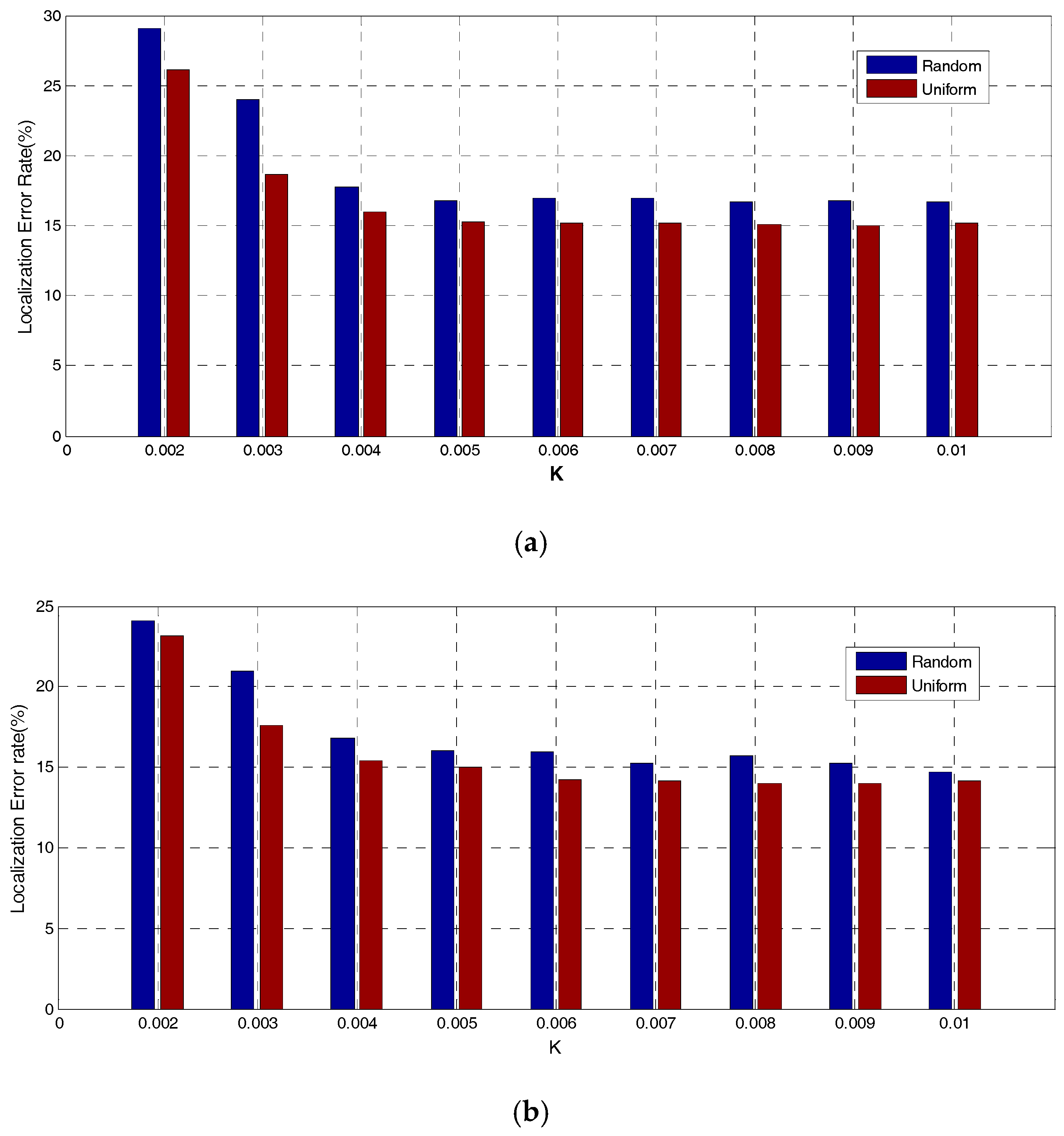
3. Localization Error Rate Varying K
In this experiment, it analyses the parameters of K that influence localization error rate. K is the proportion of triangles reduced. In the experiments, the sensor nodes distributed in random and uniform distribution respectively.
In Figure 13a, the parameters are as follows: AH = 3, AP = 20%, R = 450 m, K = 0.0020~0.01. The sensor nodes are distributed in random and uniform distribution.
Figure 13a shows that the overall trend of localization error rate in HTCRL localization algorithms decreases as K increases. When K is from 0.002 to 0.04, the localization error rate decreases dramatically. But when K is from 0.004 to 0.01, the localization error rate changes little. The localization error rate of HTCRL is about 15%. The performance is remarkable. The localization error rate of HTCRL is from 29.06% to 16.07% under the random distribution. Under the uniform distribution, the localization error rate of HTCRL is from 26.16% to 15.15% under random distribution. In general, localization error rate of HTCRL decreases when K increases gradually.
In Figure 13b, the parameters are as follows: AH = 3, AP = 30%, R = 450 m, K = 0.0020~0.01. The sensor nodes are distributed in random and uniform distribution.
Figure 13b shows that the overall trend of localization error rate in HTCRL localization algorithms decreases as K increases. When K is from 0.002 to 0.04, the localization error rate decreases dramatically. But when K is from 0.004 to 0.01, the localization error rate changes little. The localization error rate of HTCRL is about 14%. The performance is remarkable. The localization error rate of HTCRL is from 24.01% to 14.7% under the random distribution. Under the uniform distribution, the localization error rate of HTCRL is from 23.05% to 14.12% under the random distribution. In general, localization error rate of HTCRL decreases when K increases gradually.
From Figure 13, it can be seen that the localization error rate decreases significantly when K is greater than 0.004 under the two distribution. Moreover, it will decrease gradually with the increasing of R.
5. Conclusions
In this paper, we analyzed some related works about APIT localization algorithms. In view of their shortcomings, the paper proposes an improved APIT algorithm HTCRL, which is based on the principle of homothetic triangle. In order to compare the performance of these two algorithms, several experiments are done. We have considered different parameters, including random distributed network, uniform distributed network, anchors heard, node density, anchor percentage, anchor to node range ratio, and communication radius. In all these parameters, the performance of the HTCRL localization algorithm is better than the APIT algorithm without introducing additional hardware or communication overhead.
Acknowledgments
This work is supported by the Science and Technology Planning Project of Daqing under grant zd-2016-054.
Author Contributions
Dan Zhang and Zhiyi Fang conceived and designed the HTCRL localization algorithm and experiments; Hongyu Sun performed the experiments; Jie Cao analyzed the data; all authors have read and approved the final manuscript.
Conflicts of Interest
The authors declare no conflict of interest.
References
- Hoffmann, G.M.; Tomlin, C.J. Mobile sensor network control using mutual information methods and particle filters. IEEE Trans. Autom. Control 2010, 55, 32–47. [Google Scholar] [CrossRef]
- Velimirovic, A.S.; Djordjevic, G.L.; Velimirovic, M.M.; Jovanovic, M.D. Fuzzy ring-overlapping range-free (FRORF) localization method for wireless sensor networks. Comput. Commun. 2012, 35, 1590–1600. [Google Scholar] [CrossRef]
- Sun, H.; Fang, Z.; Li, Y.; Yu, Y.; Kong, S.; Sun, Y. Research and application of wireless network equipment in coal mine gas monitoring system. J. Theor. Appl. Inf. Technol. 2012, 45, 44–48. [Google Scholar]
- Sun, H.; Fang, Z.; Qu, G. CESILA: Communication Circle External Square Intersection-Based WSN Localization Algorithm. Sens. Transducers 2013, 155, 128–135. [Google Scholar]
- Girod, L.; Estrin, D. Robust range estimation using acoustic and multimodal sensing. In Proceedings of the IEEE International Conference on Intelligent Robots and Systems, Maui, HI, USA, 29 October–3 November 2001; pp. 1312–1320. [Google Scholar]
- Park, J.; Park, D. Ad-Hoc Localization Method Using Ranging and Bearing. In Proceedings of the International Conference on Information Technology Convergence and Services (ITCS-2011), Gwangju, Korea, 20–22 October 2011. [Google Scholar]
- Zhou, B.; Jing, C.; Kim, Y. Joint TOA/AOA positioning scheme with IP-OFDM systems. In Proceedings of the IEEE INFOCOM, Toronto, ON, Canada, 27 April–2 May 2014; pp. 1734–1743. [Google Scholar]
- Botai, O.J.; Combrinck, L.; Rautenbach, C.J.H. On the global geodetic observing system: Africa’s preparedness and challenges. Acta Astronaut. 2013, 83, 119–124. [Google Scholar] [CrossRef]
- Papamanthou, C.; Preparata, F.P.; Tamassia, R. Algorithms for Location Estimation Based on RSSI Sampling. In Proceedings of the ALGOSENSORS, LNCS, Reykjavik, Iceland, 12 July 2008; pp. 72–86. [Google Scholar]
- Tomic, S.; Mezei, I. Improved DV-Hop localization algorithm for wireless sensor networks. In Proceedings of the IEEE 10th Jubilee International Symposium on Intelligent Systems and Informatics, Subotica, Serbia, 20–22 September 2012; pp. 389–394. [Google Scholar]
- Zhang, B.; Ji, M. A Weighted Centroid Localization Algorithm Based on DV-Hop for Wireless Sensor Network. In Proceedings of the Conference on Wireless Communications, Networking and Mobile Computing, Shanghai, China, 21–23 September 2012; pp. 21–23. [Google Scholar]
- Huang, X.; Huang, X.; Mao, H.; Yin, Z. Iterated Hybrid Localization Algorithm for Random Wireless Sensor Networks Based on Centroid and DV-Hop Algorithm. Appl. Mech. Mater. 2012, 182, 1854–1857. [Google Scholar]
- Zhou, Y.; Ao, X.; Xia, S. An Improved APIT Node Self-localization Algorithm in WSN. In Proceedings of the 7th World Congress on Intelligent Control and Automation, Chongqing, China, 25–27 June 2008; pp. 7582–7586. [Google Scholar]
- Holopainen, S. Influence of damage on inhomogeneous deformation behavior of amorphous glassy polymers. Modeling and algorithmic implementation in a finite element setting. Eng. Fract. Mech. 2014, 117, 28–50. [Google Scholar] [CrossRef]
- Feng, X.L.; Xu, H.Y.; Li, W.; Sun, Z.Y. Centroid position algorithm of structure optical stripe in asphalt pavement test. J. Optoelectron. Laser 2014, 3, 514–520. [Google Scholar]
- Ademuwagun, A.; Fabio, V. Reach Centroid Localization Algorithm. Wirel. Sens. Netw. 2017, 9, 87–101. [Google Scholar] [CrossRef]
- He, T.; Huang, C.; Blum, B.M.; Stankovic, J.A.; Abdelzaher, T. Range-Free Localization schemes for large scale Sensor networks. In Proceedings of the 9th ACM Annual International Conference on Mobile Computing and Networking (Mobicom‘03’), San Diego, CA, USA, 14–19 September 2003; pp. 81–95. [Google Scholar]
- Kaur, R.; Malhotra, J. Comparitive Analysis of DV-Hop and APIT Localization Techniques in WSN. Int. J. Future Gener. Commun. Netw. 2016, 9, 327–344. [Google Scholar] [CrossRef]
- Sun, X.; Hu, Y.; Wang, B.; Zhang, J.; Li, T. VPIT: An Improved Range-Free Localization Algorithm Using Voronoi Diagrams for Wireless Sensor Networks. Int. J. Multimed. Ubiquitous Eng. 2015, 10, 23–34. [Google Scholar] [CrossRef]
- Liu, J.; Wang, Z.; Yao, M.; Qiu, Z. VN-APIT: Virtual nodes-based range-free APIT localization scheme for WSN. Wirel. Netw. 2016, 22, 867–878. [Google Scholar] [CrossRef]
- Sharma, R.; Malhotra, S. Approximate Point in Triangulation (APIT) based Localization Algorithm in Wireless Sensor Network. Int. J. Innov. Res. Sci. Technol. 2015, 2, 39–42. [Google Scholar]
Figure 1.
Principles of the APIT algorithm.
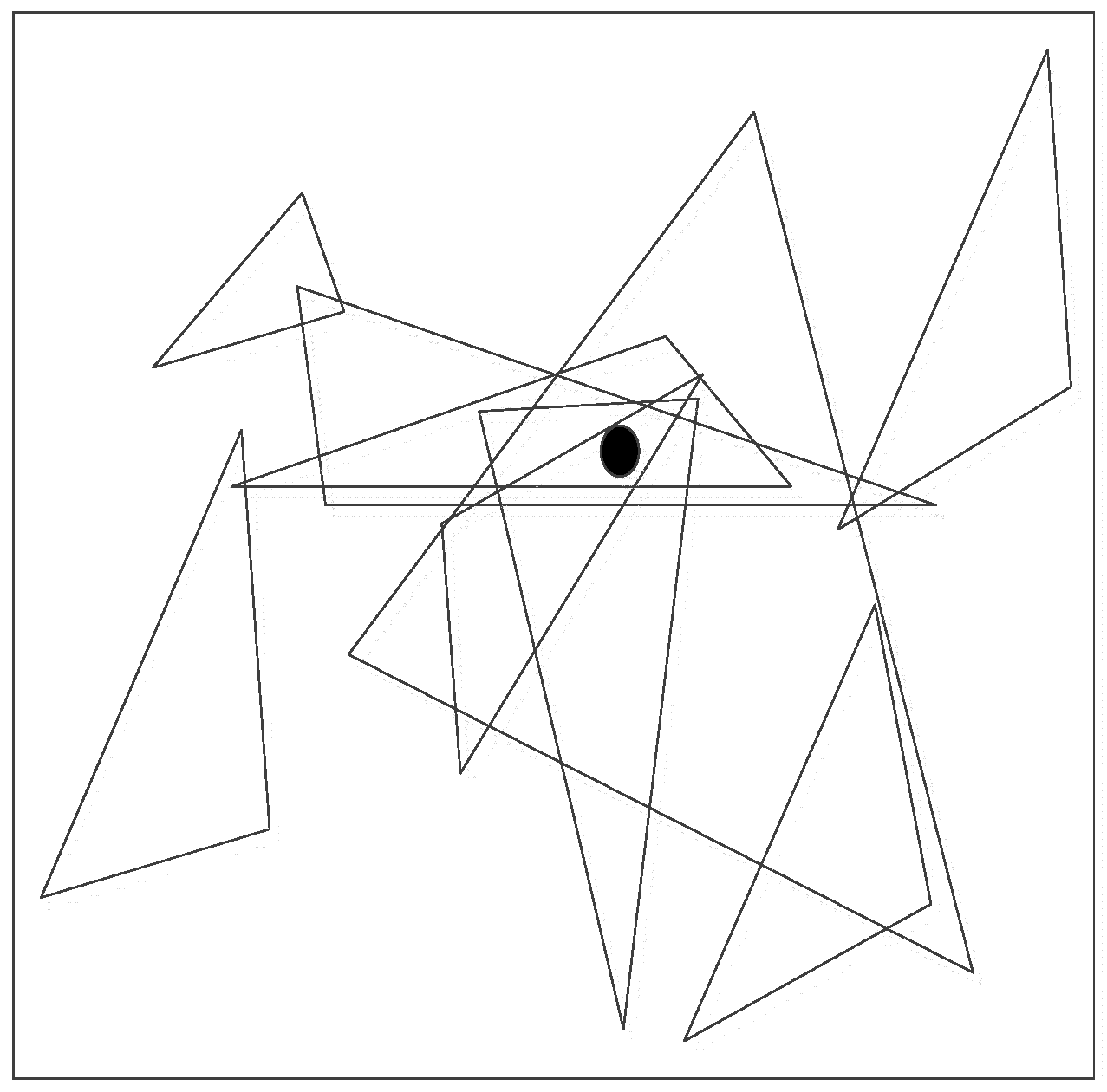
Figure 2.
The main phase of APIT.

Figure 3.
Format of the message broadcasted by anchor nodes.

Figure 4.
APIT localization test principle schematic drawing. (a) principles of PIT (unknown node in the triangle); (b) principles of PIT (unknown node out of the triangle).
Figure 4.
APIT localization test principle schematic drawing. (a) principles of PIT (unknown node in the triangle); (b) principles of PIT (unknown node out of the triangle).
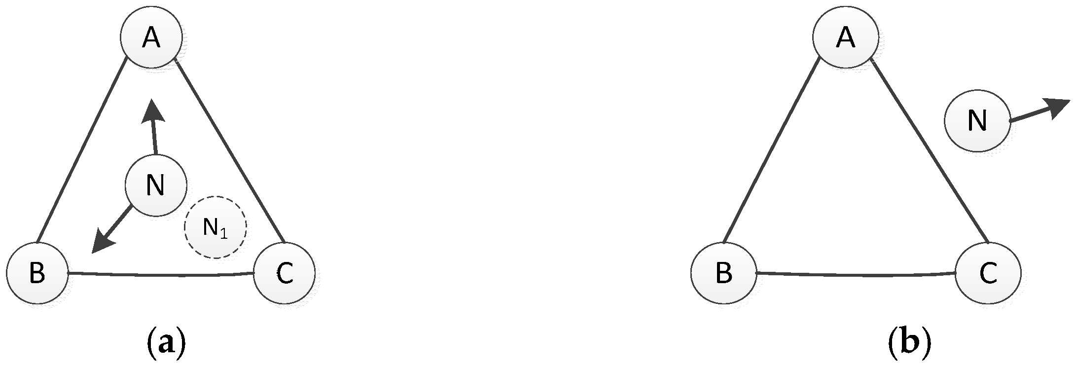
Figure 5.
APIT localization test principle schematic. (a) M is in the triangle; (b) M is out of the triangle.
Figure 5.
APIT localization test principle schematic. (a) M is in the triangle; (b) M is out of the triangle.

Figure 6.
Estimate the location of the unknown node.
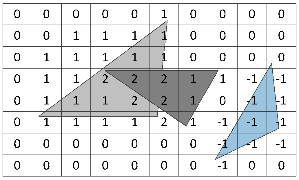
Figure 7.
The principle of homothetic triangle.

Figure 8.
Diagram of triangle’s center.
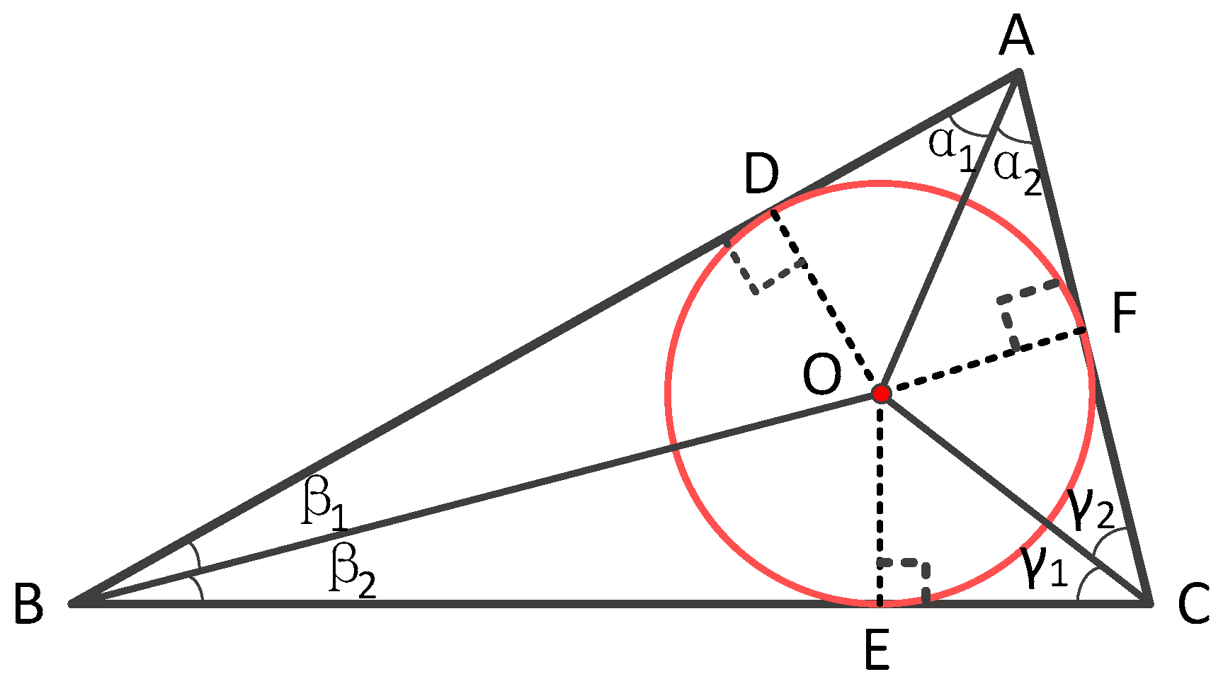
Figure 9.
The main principle of HTCRL localization algorithm.

Figure 10.
The Main Process of HTCRL Localization Algorithm.
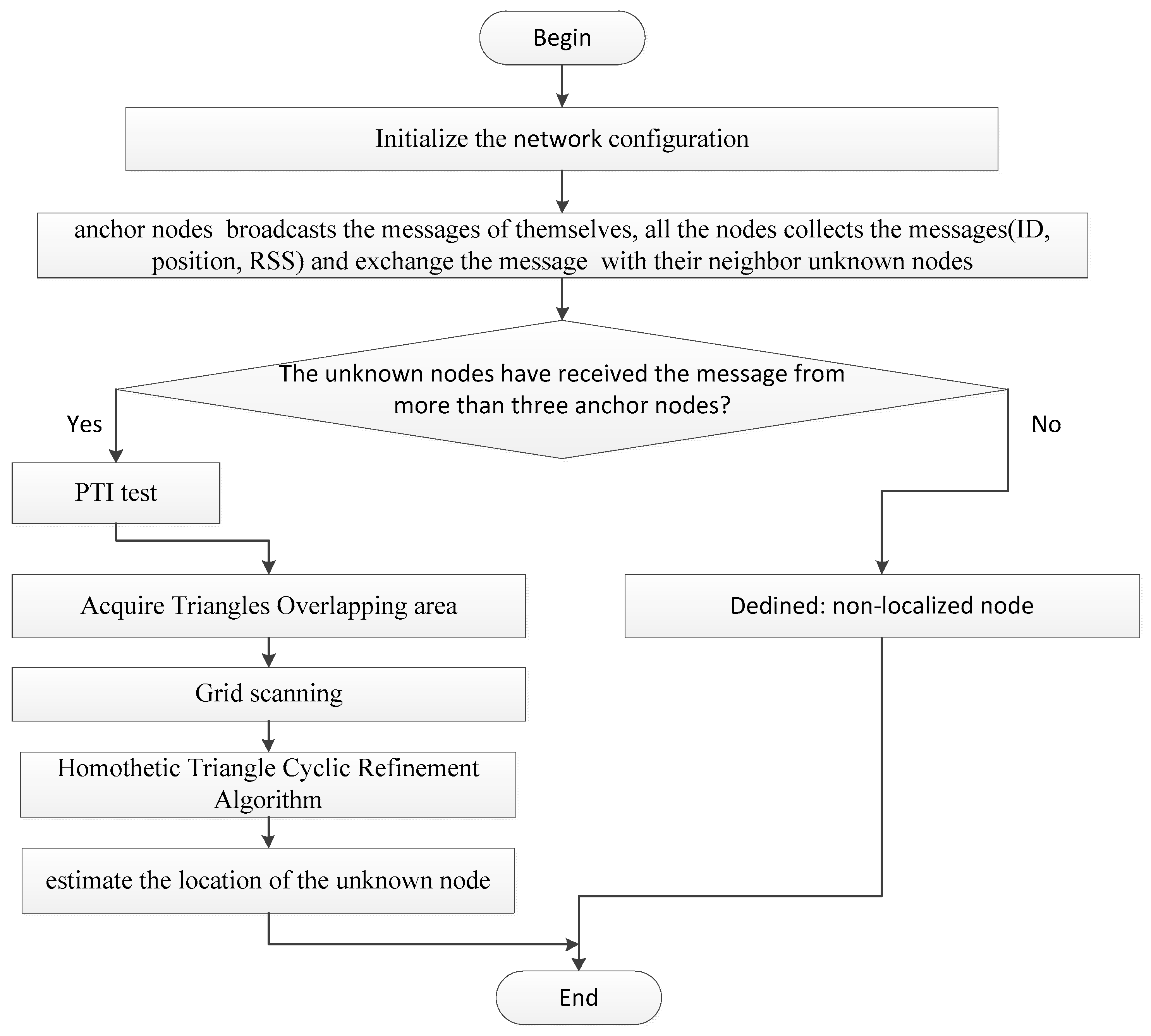
Figure 11.
Localization Error Rate Varying with Anchor Heard. (a) AH = 3~21, ANR = 3, ND = 8, R = 150, Random, K = 0.0050; (b) AH = 3~21, ANR = 3, ND = 8, R = 150, Uniform, K = 0.0050; (c) AH = 3~21, ANR = 3, ND = 8, R = 450, Random, K = 0.0050; (d) AH = 3~21, ANR = 3, ND = 8, R = 450, Uniform, K = 0.0050.
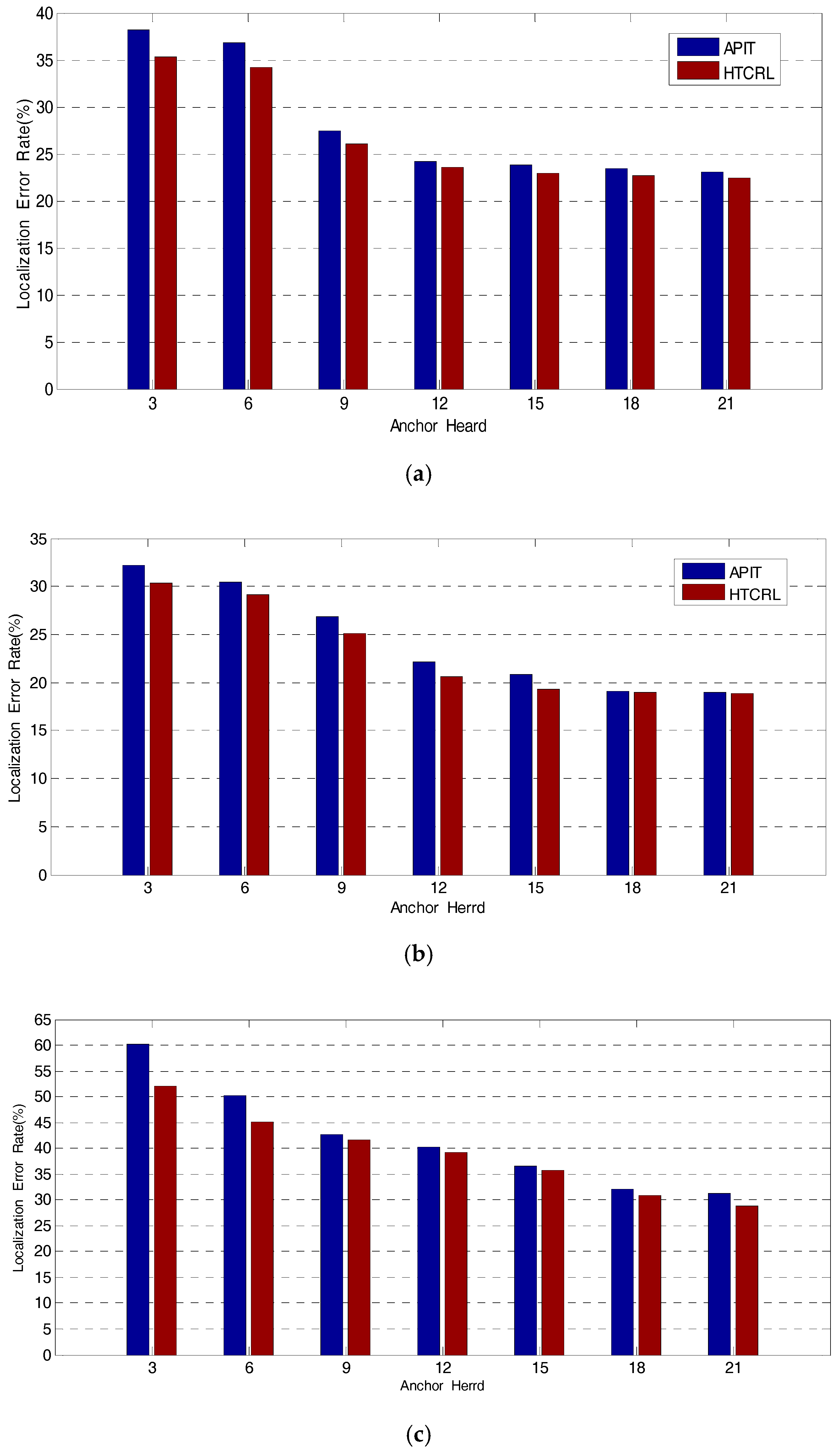

Figure 12.
Localization Error Rate Varying Node Density. (a) ND = 3~21, AH = 18, ANR = 3, AP = 20%, R = 150 m Random, K = 0.0050; (b) ND = 3~21, AH = 18, ANR = 3, AP = 30%, R = 150 m Random, K = 0.0050.
Figure 12.
Localization Error Rate Varying Node Density. (a) ND = 3~21, AH = 18, ANR = 3, AP = 20%, R = 150 m Random, K = 0.0050; (b) ND = 3~21, AH = 18, ANR = 3, AP = 30%, R = 150 m Random, K = 0.0050.
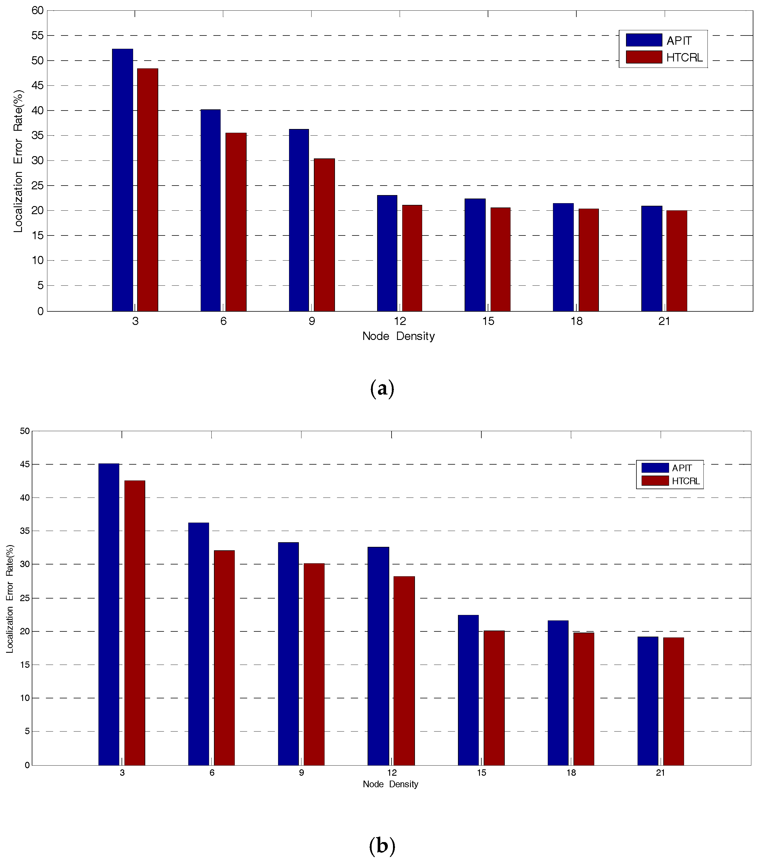
Figure 13.
Localization Error Rate Varying with K. (a) AH = 3, AP = 20%, R = 450 m, K = 0.0020~0.01; (b) AH = 3, AP = 230%, R = 450 m, K = 0.0020~0.01.
Figure 13.
Localization Error Rate Varying with K. (a) AH = 3, AP = 20%, R = 450 m, K = 0.0020~0.01; (b) AH = 3, AP = 230%, R = 450 m, K = 0.0020~0.01.

© 2017 by the authors. Licensee MDPI, Basel, Switzerland. This article is an open access article distributed under the terms and conditions of the Creative Commons Attribution (CC BY) license (http://creativecommons.org/licenses/by/4.0/).
Share and Cite
MDPI and ACS Style
Zhang, D.; Fang, Z.; Sun, H.; Cao, J. HTCRL: A Range-Free Location Algorithm Based on Homothetic Triangle Cyclic Refinement in Wireless Sensor Networks. Information 2017, 8, 40. https://doi.org/10.3390/info8020040
AMA Style
Zhang D, Fang Z, Sun H, Cao J. HTCRL: A Range-Free Location Algorithm Based on Homothetic Triangle Cyclic Refinement in Wireless Sensor Networks. Information. 2017; 8(2):40. https://doi.org/10.3390/info8020040
Chicago/Turabian StyleZhang, Dan, Zhiyi Fang, Hongyu Sun, and Jie Cao. 2017. "HTCRL: A Range-Free Location Algorithm Based on Homothetic Triangle Cyclic Refinement in Wireless Sensor Networks" Information 8, no. 2: 40. https://doi.org/10.3390/info8020040
Note that from the first issue of 2016, this journal uses article numbers instead of page numbers. See further details here.