
Object Tracking by a Combination of Discriminative Global and Generative Multi-Scale Local Models

School of Electronic and Information Engineering, South China University of Technology, No. 381, Wushan Road, Tianhe District, Guangzhou 510640, China
*
Author to whom correspondence should be addressed.
Information 2017, 8(2), 43; https://doi.org/10.3390/info8020043
Submission received: 6 February 2017
/
Revised: 5 April 2017
/
Accepted: 5 April 2017
/
Published: 11 April 2017
Abstract
:Object tracking is a challenging task in many computer vision applications due to occlusion, scale variation and background clutter, etc. In this paper, we propose a tracking algorithm by combining discriminative global and generative multi-scale local models. In the global model, we teach a classifier with sparse discriminative features to separate the target object from the background based on holistic templates. In the multi-scale local model, the object is represented by multi-scale local sparse representation histograms, which exploit the complementary partial and spatial information of an object across different scales. Finally, a collaborative similarity score of one candidate target is input into a Bayesian inference framework to estimate the target state sequentially during tracking. Experimental results on the various challenging video sequences show that the proposed method performs favorably compared to several state-of-the-art trackers.
1. Introduction
Object tracking plays an important role in the field of computer vision [1,2,3,4,5] and serves as a preprocessing step for a lot of applications in areas such as human-machine interaction [6], robot navigation [7] and intelligent transportation [8], etc. Despite significant progress that has been made in previous decades, object tracking is still a challenging task due to the changes of objects’ appearances influenced by scale variation, partial occlusion, illumination variation, and background clutter. To address these problems, it is a key issue for the success of a tracker to design a robust appearance model. Specifically, current tracking algorithms based on an object appearance model can be roughly categorized into generative, discriminative or hybrid methods.
For generative methods, the tracking problem is formulated as searching for the image regions most similar to the target model. Only the information of the target is used. In [9], an incremental subspace learning method was proposed to construct an object appearance model online within the particle filter framework. Kwon et al. [10] utilized multiple basic observation and motion models to cope with appearance and motion changes of an object. Motivated by the robustness of sparse representation in face recognition, Mei et al. [11] modeled tracking as a sparse approximation problem and the occlusion problem was addressed through a set of trivial templates. In [12], a tracking algorithm using the structural local sparse appearance model was proposed, which exploits both partial information and spatial information of the target based on an alignment-pooling method. The work in [13] presented a tracking algorithm based on the two-view sparse representation, where the tracked objects are sparsely represented by both templates and candidate samples in the current frame. To encode more information, Hu et al. [14] proposed a multi-feature joint sparse representation for object tracking.
In discriminative methods, the tracking is treated as a binary classification problem aiming to find a decision boundary that can best separate the target from the background. Unlike generative methods, the information of both the target and its background is used simultaneously. The work in [15] fused together an optic-flow-based tracker and a support vector machine (SVM) classifier. Grabner and Bischof [16] proposed an online AdaBoost algorithm to select the most discriminative features for object tracking. In [17], a multiple instance learning (MIL) framework was proposed for tracking, which learned a discriminative model by putting all ambiguous positive and negative samples into bags. Zhang et al. [18] utilized sparse measurement matrix to extract low-dimensional features, and then trained a naive Bayes classifier for tracking. Recently, Henriques et al. [19] exploited the circulant structure of the kernel matrix in an SVM for tracking. In [20], a deep metric learning-based tracker was proposed, which learns a non-linear distance metric to classify the target object and background regions using a feed-forward neural network architecture.
Hybrid methods exploit the complementary advantages of the previous two approaches. Yu et al. [21] utilized two different models for tracking, where the target appearance is described by low-dimension linear subspaces and a discriminative classifier is trained to focus on recent appearance changes. In [22], Zhong et al. developed a sparse collaborative tracking algorithm that exploits both holistic templates and local patches. Zhou et al. [23] developed a hybrid model for object tracking, where the target is represented by different appearance manifolds. The tracking method in [24] integrated the structural local sparse appearance model and the discriminative classifier with a support vector machine.
Inspired by the work in [22], a hybrid tracking method by the combination of discriminative global and generative multi-scale local models is proposed in this paper. Different from [22], we represent the object using multi-scale local sparse representation histogram in generative model, where the patch-based sparse representation histogram under different patch scales is computed separately, and exploit the collaborative strength of sparse representation histogram under different patch scales. Therefore, our tracker exploits both partial and spatial information of an object across different scales. The final similarity score of a candidate is obtained by the combination of the two models under the Bayesian inference framework. The candidate with the maximum confidence is chosen as the tracking target. Additionally, an online update strategy is adopted to adapt to the appearance changes of objects. The main flow of our tracking algorithm is shown in Figure 1.
2. Discriminative Global Model
For the global model, as in [22], an object is represented through the sparse coefficients, which are obtained by encoding the object appearance with gray features, using a holistic template set. In Section 2.1, we describe the construction of the template set, where each template is represented as a vector of gray features. Due to the redundancy of gray feature space, we present a sparse discriminative feature selection method in Section 2.2, where we extract determinative gray features that best distinguish the foreground object from the background by teaching a classifier. Finally, a confidence measure method is given in Section 2.3.
2.1. Construction of the Template Set
Given the initial target region in the first frame, we sample foreground templates around the target location, as well as background templates within an annular region some pixels away from the target object. Then, the selected templates are normalized to the same size (32 × 32 in our experiments). In this way, the normalized templates are stacked together to form a template matrix , where K is the dimension of gray features, and we denote A =, i.e., for foreground templates and for background templates.
2.2. Sparse Discriminative Feature Selection
Due to the redundancy of gray feature space, we extract determinative gray features that best distinguish the foreground object from the background by teaching a classifier:
where each element of the vector represents the property of each template in the training template set A (+1 corresponds to a foreground template and −1 corresponds to a background template), and denote and norms, respectively, and is a regularization parameter. The solution of Equation (1) is the vector s , whose non-zero elements correspond to sparse discriminative features selected from the K dimensional gray feature space.
During the tracking process, the gray features in original space are projected to a discriminative subspace by a projection matrix S, which is obtained by removing all-zero rows from a diagonal matrix . In addition, the elements of diagonal matrix are obtained by:
thus, the training template set and candidates in the projected space are and .
2.3. Confidence Measure
Given a candidate , it can be represented as a linear combination of the training template set by solving:
where is the sparse coefficients, is the projected vector of x, and is a regularization parameter. The candidate with smaller reconstruction error using the foreground templates indicates it is more likely to be a target, and vice versa. Thus, the confidence value of the candidate target x is formulated by:
where is the reconstruction error of the candidate x using the foreground templates and is the sparse coefficient vector corresponding to the foreground templates. is the reconstruction error of the candidate x using the background templates , and α− is the sparse coefficient vector corresponding to the background templates. The variable is a fixed constant.
3. Generative Multi-Scale Local Model
In [22], an object is represented by the patch-based sparse representation histogram with only a fixed-patch scale in the generative model. In order to decrease the impact of the patch size, a generative multi-scale local model is proposed in our work. We represent the object using multi-scale sparse representation histogram, where the patch-based sparse representation histogram under different patch scales is computed separately, and exploit the collaborative strength of sparse representation histogram under different patch scales. Moreover, we compute the similarity of histograms between the candidate and the template for each patch scale separately, and then weigh them as the final similarity measure between the candidate and the template. The illustration of the proposed multi-scale local model is shown in Figure 2.
3.1. Multi-Scale Sparse Representation Histogram
Give a target object, we normalize it to 32 × 32 pixels. Then, the object is segmented hierarchically into three layers, and each layer consists of local patches with different patch scales. Three scales with patch sizes 4 × 4, 6 × 6, and 9 × 9 are used in our work. For simplicity, the gray features are used to represent the patch information of a target object. The local patches of each scale are collected by a sliding window with the corresponding scale and the step length in the sampling process being the same as two pixels. Assume that is the vectorized local patches extracted from a target candidate under different patch scales, where denotes the i-th local patch under patch scale k, is the dimensionality of local patch, and is the number of local patches for scale k. The dictionary under different patch scales is , where is the number of dictionaries for scale k. The dictionary is generated by the k-means algorithm and only comes from patches of the target region manually labeled in the first frame. With the dictionary, each has a corresponding sparse coefficient , which can be obtained by solving an - regularized least-squares problem:
where λ3 is a regularization parameter.
When the sparse coefficients of all local patches of one candidate are computed under different patch scales, they are normalized and concatenated to form a sparse representation histogram by:
where is the spare representation histogram for one candidate under patch scale k. Then, the candidate is represented with the combination of multiple scale histograms.
3.2. Histogram Modification
During the tracking process, the target’s appearance changes significantly due to outliers (such as noise or occlusion). To address the issue, we modify the sparse representation histogram to exclude the corrupted patch. The corrupted patch usually has a large reconstruction error and its sparse coefficient vector is set to be zero. Thus, the modified histogram under different scales can be obtained by:
where denotes the element-wise multiplication. Each element of is a descriptor for corrupted patch and is defined by:
where represents the reconstruction error of local patch , and is a threshold indicating whether the patch is corrupted or not. We, thus, have constructed the sparse representation histogram under different scales, which exploits multi-scale information of the target and takes outliers into account.
3.3. Similarity Measure
The key issue in object tracking is the determination of the similarity between the candidate and the template. We use the histogram intersection function to compute the similarity of histograms between the candidate and the template for each patch scale separately, and then weigh them as the final similarity measure between the candidate and the template, which is computed by:
where and are the histograms for the template and the c-th candidate under patch scale k, and is a weight used to measure the outlier under patch scale k. Moreover, is defined by:
The template histograms under different patch scales are generated by Equations (5)–(7) and computed only once for each tracking sequence. When evaluating the similarity of histograms between the candidate and the template, we modify the template histograms under the same condition as modifying the histograms of the candidate.
4. Tracking by Bayesian Inference
Object tracking can be treated as a Bayesian inference task [25]. Given the observations of target up to time t, the current target state can be obtained by the maximum a posteriori estimation via:
where denotes the i-th sample of the state . The posterior probability can be recursively computed by the Bayesian theorem via:
where and denote the dynamic model and observation model, respectively. The dynamic model describes the temporal correlation of the target states in consecutive frames, and the motion of the target between consecutive frames is modeled by an affine transformation. The state transition is formulated by random walk, i.e., , where denote the x, y translations, scale and aspect ratio at time t, respectively. is a diagonal covariance matrix whose elements are the variances of the affine parameters.
The observation model estimates the likelihood of observing at state . In this paper, the collaborative likelihood of the c-th candidate is defined as:
and the candidate with the maximum likelihood value is regarded as the tracking result.
5. Online Update
In order to adapt the change of target appearance during tracking, the update scheme is essential. The global model and multi-scale local model are updated independently. For the global model, the negative templates are updated every five frames and the positive templates remain the same during tracking. As the global model aims to select sparse discriminative feature to separate the target object from the background, it is important to ensure that the positive and negative templates are all correct and distinct.
For the multi-scale local model, the dictionary for each scale is fixed to ensure that the dictionary is not affected even if outliers occur during tracking. In order to capture the change of the target’s appearance and balance between the old and new templates, the new template histogram under patch scales k is computed by:
where is the histogram at the first frame, denotes the histogram last frame before update, and are the weight, the variable defined by Equation (10) is the outlier measure for scale k in the current frame, and is a predefined constant.
6. Experiments
We evaluate our tracking algorithm on 12 public video sequences from the benchmark dataset [26]. These sequences include different challenging situations like occlusion, scale variation, cluttered background, and illumination changes. Our tracker is compared with several state-of-the-art trackers, including tracking-learning-detection method (TLD) [27], structured output tracker (STRUCK) [28], tracking via sparse collaborative appearance model (SCM) [22], tracker with multi-task sparse learning (MTT) [29] and tracking with kernelized correlation filters (KCF) (with histogram of oriented gradient features) [19]. We implement the proposed method in MATLAB 2013a (The MathWorks, Natick, MA, USA) on a PC with Intel G1610 CPU (2.60 GHz) with 4 GB memory. For fair comparisons, we use the source code provided by the benchmark [26] with the same parameters, except KCF. We run the KCF with the default parameters reported in the corresponding paper.
The parameters of our tracker for all test sequences are fixed to demonstrate its robustness and stability. We manually label the location of the target in the first frame for each sequence. The number of particles is 300 and the variance matrix of affine parameters is set as Σ = diag (4, 4, 0.01, 0.005). The numbers of positive templates, p, and negative templates, n, are 50 and 200, respectively.
The regularization parameters of Equations (3) and (5) are set to be 0.01, and the variable λ2 in Equation (1) is fixed to be 0.001. The dictionary size for each scale is 50. The threshold in Equation (8) is 0.04. The parameters , and in Equation (14) are set to 0.8, 0.85 and 0.95.
6.1. Quantitative Comparison
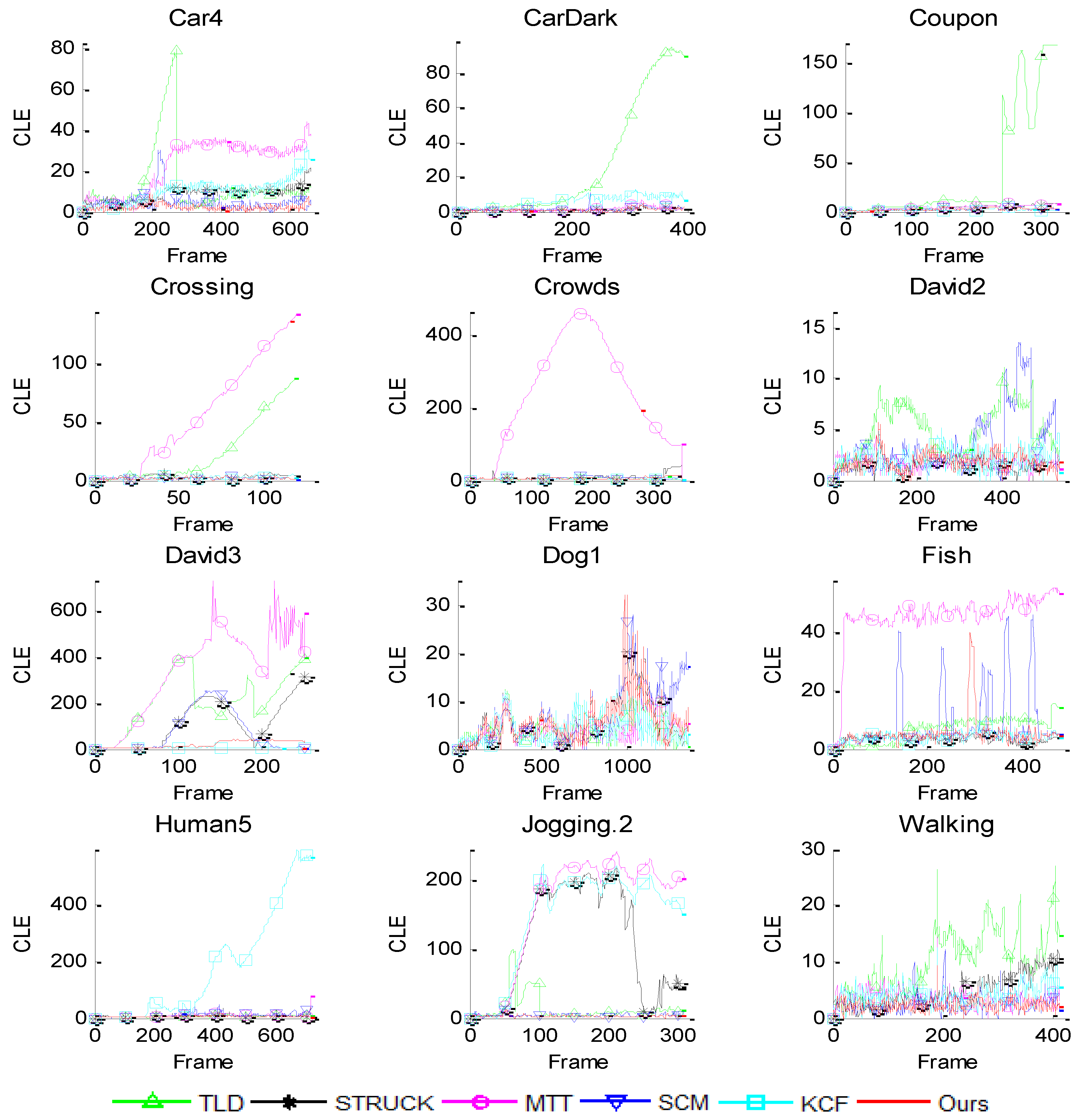
We quantitatively evaluate the performance of each tracker in terms of the center location error (CLE) and the overlap rate, as well their average values. The CLE measures the Euclidean distance between the center of the tracking result and the ground truth, and is defined as , where and denote the tracked central position and ground truth central position, respectively. The lower CLE will result in the better performance. The overlap rate reflects stability of each tracker as it takes the size and pose of the target object into account. It is defined by PASCAL VOC criteria [30], score = , where is the tracking bounding box and is the ground truth bounding box. More accurate trackers have higher overlap rates. Figure 3 shows the frame-by-frame center location error comparison results. Table 1 and Table 2 report the comparison results of our tracker and five other trackers in terms of average CLE and average overlap rate. In both tables, the first row gives all of the trackers and the first column shows all the videos in our experiment. The last row is the average of the results for each tracker.
As shown in Figure 3, the CLE curves diverge for some trackers, such as the TLD tracker in the CarDark, Coupon, Crossing and David3 video sequences, the STRUCK tracker in the David3 and Jogging.2 video sequences, the KCF tracker in the Human5 and Jogging.2 video sequences, etc. These indicate that these trackers lose the tracking objects in the tracking process. From Table 1 and Table 2, we can see that our tracker achieves the best or second-best performances. Moreover, our tracker obtains the best performance for 12 video sequences when compared with the SCM tracker, and this suggests that the multi-scale local information adopted in our model is very effective and important for tracking. Overall, our tracker performs favorably against the other five state-of-the-art algorithms with lower center location errors and higher overlap rates.
6.2. Qualitative Comparison
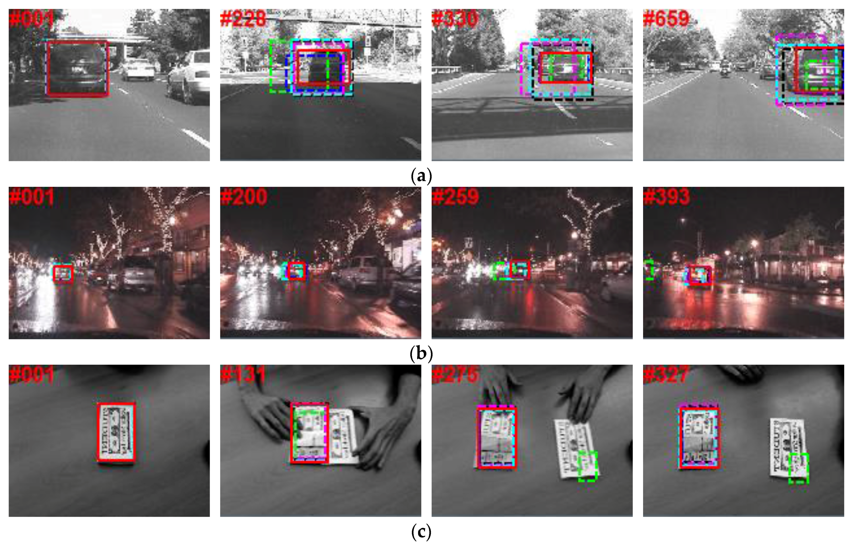
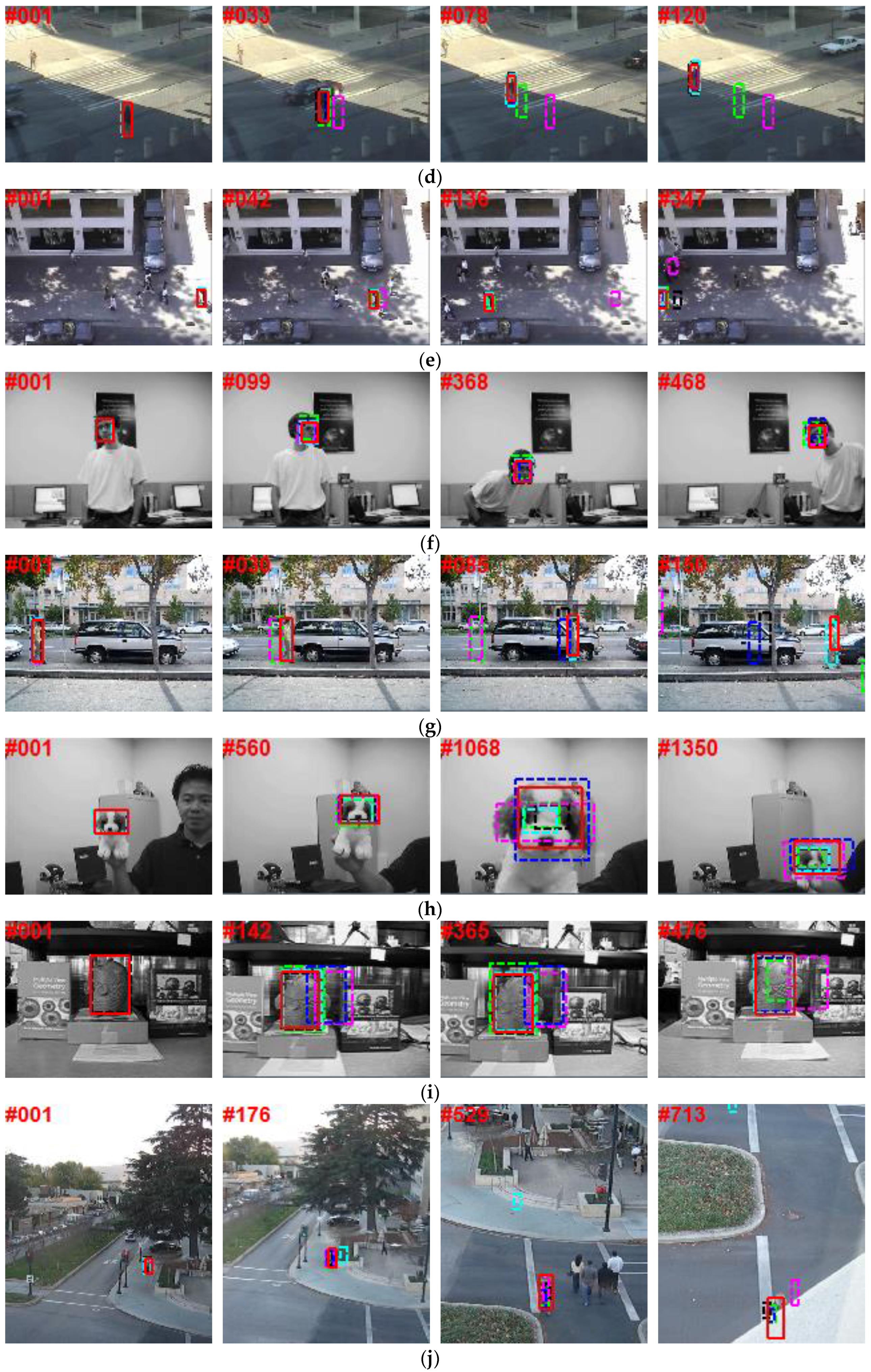
To further evaluate the performance of our tracker against the other state-of-art trackers, several screenshots of the tracking results on 12 video sequences [26] are shown in Figure 4. For these sequences, several principal factors that have effects on the appearance of an object are considered. Some other factors are also included in the discussion. Qualitative discussion is detailed below.
Illumination Variation: Figure 4a,i present tracking results of two challenging sequences with illumination variation to verify the effectiveness of our tracker. In the Car4 sequence, the TLD tracker severely deviates from the object location when the car goes below the bridge creating a dramatic illumination change (e.g., frame 228). The MTT tracker shows a severe drift when the car becomes smaller. The SCM tracker and our tracker can track the target accurately. For the Fish sequence, illumination changes and camera movement makes it challenging. All trackers, except MTT and SCM, work well.
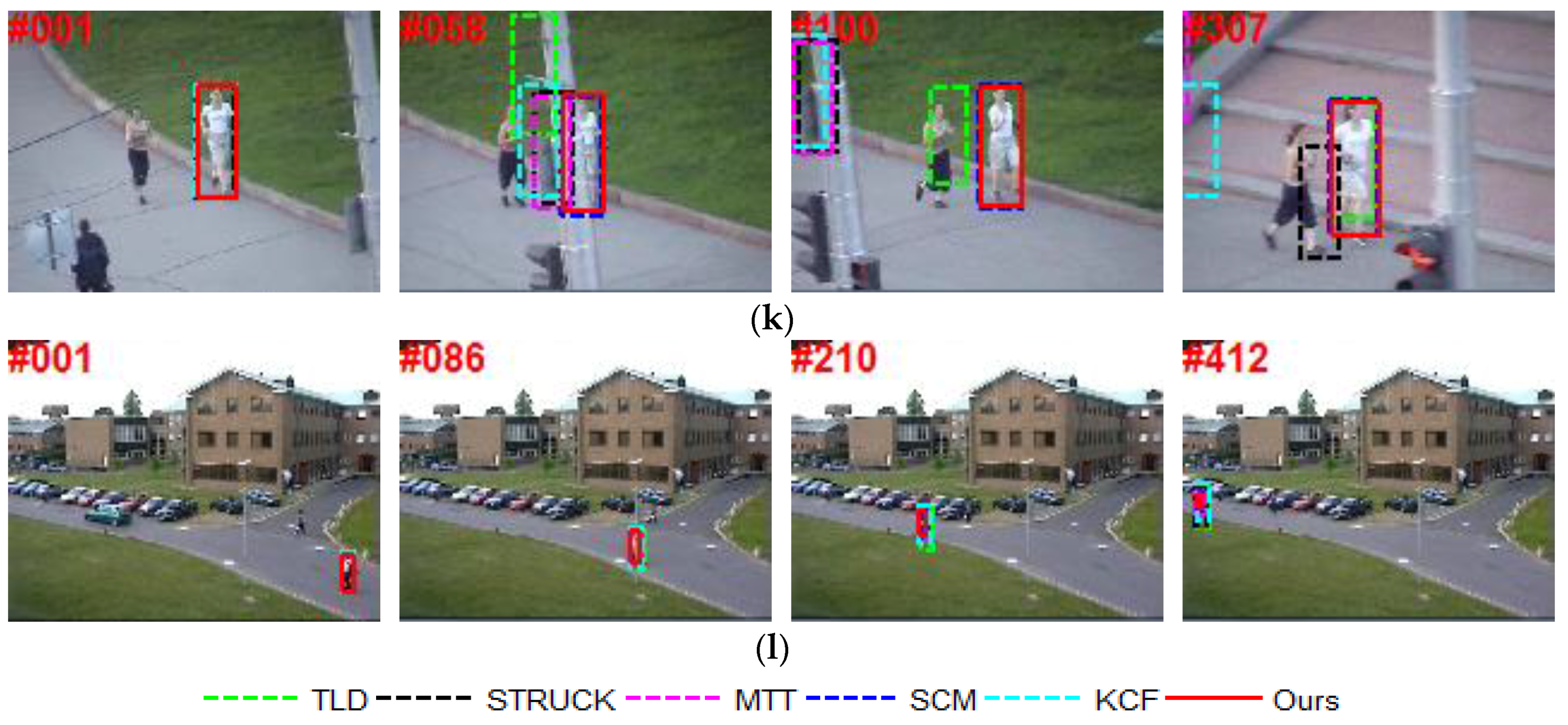
Occlusion: Occlusion is one of the most general, yet crucial, problems in object tracking. In the David3 sequence (Figure 4g), severe occlusion is introduced by tree and object appearance changes drastically when the man turns around. Only the KCF and our tracker successfully locate the correct object throughout the sequence. For the Jogging.2 sequence (Figure 4k), when the girl is occluded by the pole (e.g., frame 58), all of the other trackers drift away from the target object, except for SCM and our track.
Background Clutter: The CarDark sequence in Figure 4b shows a moving vehicle at night with dramatic illumination changes and low contrast in cluttered background. The TLD tracker starts to drift around frame 200 and gradually losses the target. Other trackers can track the car accurately.
For the Coupon sequence (Figure 4c, the tracked object is the uppermost coupon and an imposter coupon book similar to the target is introduced to distract the trackers. The KCF and our trackers perform better. In the Crowds sequence (Figure 4e, the target is a man who walked from right to left. All trackers, except STRUCK and MTT, are able to track the whole sequence successfully, and the MTT tracker starts to drift around frame 42 when an object of similar color is in proximity to the tracked target.
Scale Variation and Deformation: For the Crossing sequence, all trackers, except TLD and MTT, can reliably track the object, as shown in Figure 4d. In the Human5 sequence (Figure 4j), our tracker gives the best result. The KCF and MTT trackers lose the target. Figure 4l shows the tracking results in the Walking sequence. Our tracker achieves the best performance, followed by the SCM tracker.
Rotation: The David2 sequence consists of both in-plane and out-of-plane rotations. We can see from Figure 4f that the accuracy of our tracker is higher than the accuracy of the SCM trackers. As is illustrated in Dog1 (Figure 4h), the target in this sequence undergoes both in-plane and out-of-plane rotations, and scale variation. Our tracker gives the best result in terms of the overlap rate.
7. Conclusions
In this paper, we present a robust object tracking approach by combining discriminative global and generative multi-scale local models. In the global appearance model, a classifier with sparse discriminative features is taught to separate the target object from the background. In the multi-scale local appearance model, the appearance of an object is modeled by multi-scale local sparse representation histograms. Therefore, compared with SCM tracker, our tracker could utilize both partial and spatial information of an object across different scales, which are mutually complementary. The final similarity score of a candidate is obtained by the combination of the two models under the Bayesian inference framework. Additionally, an online update strategy is adopted to adapt to the appearance changes of object. Extensive experiments on several challenging video sequences demonstrate the effectiveness and robustness of the proposed tracker.
Acknowledgments
The authors would like to thank the editors and the anonymous referees for their valuable comments and suggestions.
Author Contributions
Zhiguo Song designed the presented object tracking algorithm and wrote the paper; Jialin Yue revised the paper; and Jifeng Sun supervised the work.
Conflicts of Interest
The authors declare no conflict of interest.
References
- Li, X.; Hu, W.M.; Shen, C.H.; Zhang, Z.F.; Dick, A.; Hengel, A.V.D. A Survey of Appearance Models in Visual Object Tracking. ACM Trans. Intell. Syst. Technol. 2013, 4, 58. [Google Scholar] [CrossRef]
- Fu, H.; Duan, R.; Kircali, D.; Kayacan, E. Onboard Robust Visual Tracking for UAVs Using a Reliable Global-Local Object Model. Sensors 2016, 16, 1406. [Google Scholar] [CrossRef] [PubMed]
- Du, D.; Zhang, L.; Lu, H.; Mei, X.; Li, X. Discriminative Hash Tracking With Group Sparsity. IEEE Trans. Cybern. 2016, 46, 1914–1925. [Google Scholar] [CrossRef] [PubMed]
- Wang, J.; Zhang, J. Robust Object Tracking in Infrared Video via Adaptive Weighted Patches. Math. Comput. Appl. 2017, 22, 3. [Google Scholar] [CrossRef]
- Ruan, Y.; Wei, Z. Real-Time Visual Tracking through Fusion Features. Sensors 2016, 16, 949. [Google Scholar] [CrossRef] [PubMed]
- Krafka, K.; Khosla, A.; Kellnhofer, P.; Kannan, H. Eye Tracking for Everyone. In Proceedings of the IEEE Conference on Computer Vision and Pattern Recognition (CVPR), Las Vegas, NV, USA, 26 June–1 July 2016; pp. 2176–2184. [Google Scholar]
- Monajjemi, M.; Mohaimenianpour, S.; Vaughan, R. UAV, Come To Me: End-to-End, Multi-Scale Situated HRI with an Uninstrumented Human and a Distant UAV. In Proceedings of the International Conference on Intelligent Robots and Systems (IROS), Daejeon, Korea, 9–14 October 2016; pp. 4410–4417. [Google Scholar]
- Kwak, J.Y.; Ko, B.C.; Nam, J.Y. Pedestrian Tracking Using Online Boosted Random Ferns Learning in Far-Infrared Imagery for Safe Driving at Night. IEEE Trans. Intell. Transp. Syst. 2017, 18, 69–80. [Google Scholar] [CrossRef]
- Ross, D.A.; Lim, J.; Lin, R.S.; Yang, M.H. Incremental Learning for Robust Visual Tracking. Int. J. Comput. Vis. 2008, 77, 125–141. [Google Scholar] [CrossRef]
- Kwon, J.; Lee, K.M. Visual Tracking Decomposition. In Proceedings of the IEEE Conference on Computer Vision and Pattern Recognition (CVPR), San Francisco, CA, USA, 13–18 June 2010; pp. 1269–1276. [Google Scholar]
- Mei, X.; Ling, H. Robust Visual Tracking using L1 Minimization. In Proceedings of the International Conference on Computer Vision (ICCV), Kyoto, Japan, 29 September–2 October 2009; pp. 1436–1443. [Google Scholar]
- Jia, X.; Lu, H.; Yang, M.H. Visual Tracking via Adaptive Structural Local Sparse Appearance Model. In Proceedings of the IEEE Conference on Computer Vision and Pattern Recognition (CVPR), Providence, RI, USA, 16–21 June 2012; pp. 1822–1829. [Google Scholar]
- Wang, D.; Lu, H.; Bo, C. Online Visual Tracking via Two View Sparse Representation. IEEE Signal Process. Lett. 2014, 21, 1031–1034. [Google Scholar]
- Hu, W.; Li, W.; Zhang, X.; Maybank, S. Single and Multiple Object Tracking Using a Multi-Feature Joint Sparse Representation. IEEE Trans. Pattern Anal. Mach. Intell. 2015, 37, 816–833. [Google Scholar] [CrossRef] [PubMed]
- Avidan, S. Support Vector Tracking. IEEE Trans. Pattern Anal. Mach. Intell. 2004, 26, 1064–1072. [Google Scholar] [CrossRef] [PubMed]
- Grabner, H.; Bischof, H. On-line Boosting and Vision. In Proceedings of the IEEE Conference on Computer Vision and Pattern Recognition (CVPR), New York, NY, USA, 17–22 June 2006; pp. 260–267. [Google Scholar]
- Babenko, B.; Yang, M.H.; Belongie, S. Visual Tracking with Online Multiple Instance Learning. In Proceedings of the IEEE Conference on Computer Vision and Pattern Recognition (CVPR), Miami, FL, USA, 20–25 June 2009; pp. 983–990. [Google Scholar]
- Zhang, K.; Zhang, L.; Yang, M.H. Real-time compressive tracking. In Proceedings of the European Conference on Computer Vision (ECCV), Florence, Italy, 7–13 October 2012; pp. 864–877. [Google Scholar]
- Henriques, J.F.; Caseiro, R.; Martins, P.; Batista, J. High-Speed Tracking with Kernelized Correlation Filters. IEEE Trans. Pattern Anal. Mach. Intell. 2015, 37, 583–596. [Google Scholar] [CrossRef] [PubMed]
- Hu, J.; Lu, J.; Tan, Y.P. Deep Metric Learning for Visual Tracking. IEEE Trans. Circuits Syst. Video Technol. 2016, 26, 2056–2068. [Google Scholar] [CrossRef]
- Yu, Q.; Dinh, B.T.; Medioni, G. Online Tracking and Reacquisition Using Co-trained Generative and Discriminative Trackers. In Proceedings of the European Conference on Computer Vision (ECCV), Marseille, France, 12–18 October 2008; pp. 678–691. [Google Scholar]
- Zhong, W.; Lu, H.; Yang, M.H. Robust Object Tracking via Sparse Collaborative Appearance Model. IEEE Trans. Image Process. 2014, 23, 2356–2368. [Google Scholar] [CrossRef] [PubMed]
- Zhou, T.; Lu, Y.; Di, H. Locality-Constrained Collaborative Model for Robust Visual Tracking. IEEE Trans. Circuits Syst. Video Technol. 2015, 27, 313–325. [Google Scholar] [CrossRef]
- Dou, J.; Qin, Q.; Tu, Z. Robust Visual Tracking Based on Generative and Discriminative Model Collaboration. Multimed. Tools Appl. 2016. [Google Scholar] [CrossRef]
- Wang, D.; Lu, H.; Yang, M.H. Online Object Tracking with Sparse Prototypes. IEEE Trans. Image Process. 2013, 22, 314–325. [Google Scholar] [CrossRef] [PubMed]
- Wu, Y.; Lim, J.; Yang, M.H. Object Tracking Benchmark. IEEE Trans. Pattern Anal. Mach. Intell. 2015, 37, 1834–1848. [Google Scholar] [CrossRef] [PubMed]
- Kalal, Z.; Matas, J.; Mikolajczyk, K. P-N Learning: Bootstrapping Binary Classifiers by Structural Constraints. In Proceedings of the IEEE Conference on Computer Vision and Pattern Recognition (CVPR), San Francisco, CA, USA, 13–18 June 2010; pp. 49–56. [Google Scholar]
- Hare, S.; Saffari, A.; Torr, P. Struck: Structured Output Tracking with Kernels. In Proceedings of the International Conference on Computer Vision (ICCV), Barcelona, Spain, 6–13 November 2011; pp. 263–270. [Google Scholar]
- Zhang, T.; Ghanem, B.; Liu, S.; Ahuja, N. Robust visual tracking via multi-task sparse learning. In Proceedings of the IEEE Conference on Computer Vision and Pattern Recognition (CVPR), Providence, RI, USA, 16–21 June 2012; pp. 2042–2049. [Google Scholar]
- Everingham, M.; Gool, L.V.; Williams, C.; Winn, J.; Zisserman, A. The PASCAL Visual Object Classes (VOC) Challenge. Int. J. Comput. Vis. 2010, 88, 303–338. [Google Scholar] [CrossRef]
Figure 1.
The main flow of our tracking algorithm.
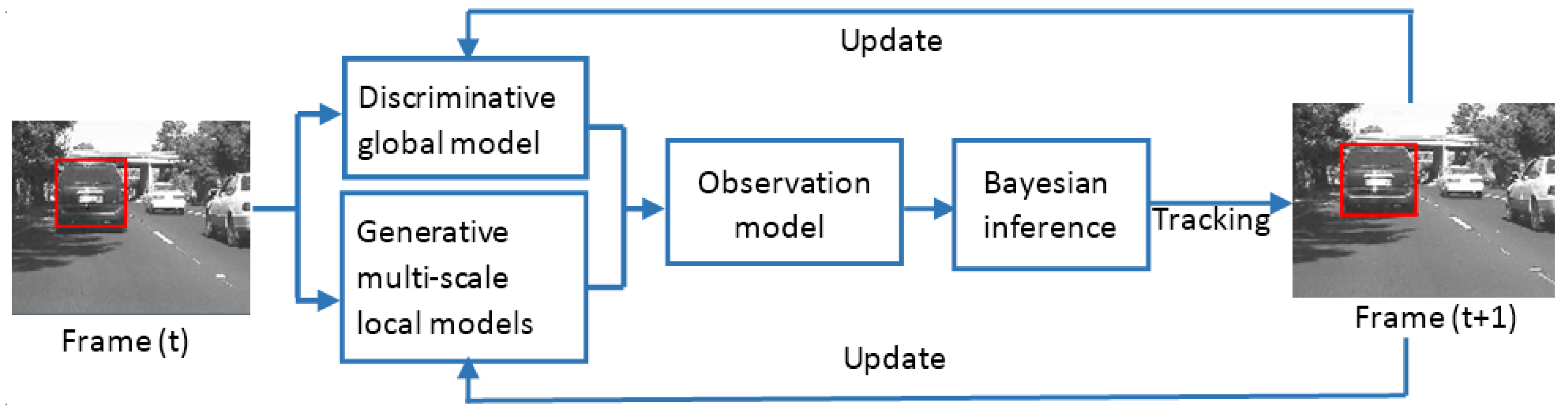
Figure 2.
An illustration of generative multi-scale local model. (a) A candidate; (b) sampling patches under different patch scales; (c) sparse representation histograms of the candidate under different patch scales; (d) modifying the histograms of the candidate excluding the outlier patches; (e) computing the similarity of histograms between the candidate and the template for each patch scale separately; (f) weighing the similarity of histograms of different patch scales as the final similarity measure between the candidate and the template.
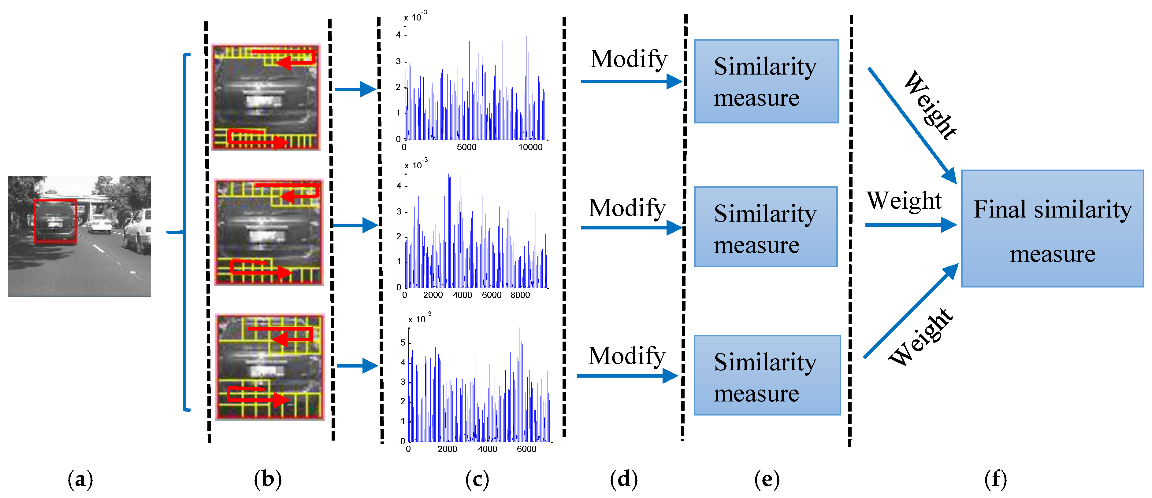
Figure 3.
Frame-by-frame comparison of six trackers in terms of center location error (CLE).

Figure 4.
Screenshots of some sampled tracking results. (a) Car4 with illumination and scale variation; (b) CarDark with illumination variation and background clutter; (c) Coupon with occlusion and background clutter; (d) Crossing with scale variation and deformation; (e) Crowds with illumination variation and background clutter; (f) David2 with in-plane rotation and out-of-plane rotation; (g) David3 with occlusion and deformation; (h) Dog1 with scale variation and rotation; (i) Fish with illumination variation; (j) Human5 with scale variation and deformation; (k) Jogging.2 with occlusion and deformation; (l) Walking with scale variation and deformation.


Table 1.
Comparison of results in terms of average CLE (pixels). Bold fonts indicate the best performance while the italic fonts indicate the second best ones.
Table 1.
Comparison of results in terms of average CLE (pixels). Bold fonts indicate the best performance while the italic fonts indicate the second best ones.
| Sequence | TLD | STRUCK | MTT | KCF | SCM | Ours |
|---|---|---|---|---|---|---|
| Car4 | 12.84 | 8.69 | 22.34 | 9.88 | 4.27 | 2.09 |
| CarDark | 27.47 | 0.95 | 1.57 | 6.05 | 1.30 | 1.04 |
| Coupon | 38.41 | 4.14 | 4.24 | 1.57 | 2.37 | 2.12 |
| Crossing | 24.34 | 2.81 | 57.15 | 2.25 | 1.57 | 1.48 |
| Crowds | 3.44 | 7.19 | 235.75 | 3.05 | 5.25 | 5.06 |
| David2 | 4.98 | 1.50 | 1.70 | 2.08 | 3.41 | 1.78 |
| David3 | 208.00 | 106.50 | 341.33 | 4.30 | 73.09 | 19.09 |
| Dog1 | 4.19 | 5.66 | 4.28 | 4.23 | 7.00 | 5.56 |
| Fish | 6.54 | 3.40 | 45.50 | 4.08 | 8.54 | 5.15 |
| Human5 | 5.31 | 6.87 | 8.28 | 175.50 | 9.33 | 4.35 |
| Jogging.2 | 13.56 | 107.69 | 157.12 | 144.47 | 4.15 | 2.46 |
| Walking | 10.23 | 4.62 | 3.47 | 3.97 | 2.49 | 2.26 |
| Average | 29.94 | 21.67 | 73.56 | 30.12 | 10.23 | 4.37 |
Table 2.
Comparison results in terms of average overlap rate. Bold fonts indicate the best performance while the italic fonts indicate the second best ones.
Table 2.
Comparison results in terms of average overlap rate. Bold fonts indicate the best performance while the italic fonts indicate the second best ones.
| Sequence | TLD | STRUCK | MTT | KCF | SCM | Ours |
|---|---|---|---|---|---|---|
| Car4 | 0.63 | 0.49 | 0.45 | 0.48 | 0.76 | 0.77 |
| CarDark | 0.45 | 0.90 | 0.83 | 0.62 | 0.84 | 0.86 |
| Coupon | 0.57 | 0.88 | 0.87 | 0.94 | 0.90 | 0.91 |
| Crossing | 0.40 | 0.68 | 0.20 | 0.71 | 0.78 | 0.80 |
| Crowds | 0.77 | 0.61 | 0.09 | 0.79 | 0.63 | 0.66 |
| David2 | 0.69 | 0.87 | 0.86 | 0.83 | 0.75 | 0.84 |
| David3 | 0.10 | 0.29 | 0.10 | 0.77 | 0.40 | 0.59 |
| Dog1 | 0.59 | 0.55 | 0.69 | 0.55 | 0.70 | 0.72 |
| Fish | 0.81 | 0.86 | 0.17 | 0.84 | 0.75 | 0.81 |
| Human5 | 0.54 | 0.35 | 0.42 | 0.18 | 0.44 | 0.72 |
| Jogging.2 | 0.66 | 0.20 | 0.13 | 0.12 | 0.73 | 0.77 |
| Walking | 0.45 | 0.57 | 0.67 | 0.53 | 0.71 | 0.71 |
| Average | 0.56 | 0.6 | 0.46 | 0.61 | 0.70 | 0.76 |
© 2017 by the authors. Licensee MDPI, Basel, Switzerland. This article is an open access article distributed under the terms and conditions of the Creative Commons Attribution (CC BY) license (http://creativecommons.org/licenses/by/4.0/).
Share and Cite
MDPI and ACS Style
Song, Z.; Sun, J.; Yu, J. Object Tracking by a Combination of Discriminative Global and Generative Multi-Scale Local Models. Information 2017, 8, 43. https://doi.org/10.3390/info8020043
AMA Style
Song Z, Sun J, Yu J. Object Tracking by a Combination of Discriminative Global and Generative Multi-Scale Local Models. Information. 2017; 8(2):43. https://doi.org/10.3390/info8020043
Chicago/Turabian StyleSong, Zhiguo, Jifeng Sun, and Jialin Yu. 2017. "Object Tracking by a Combination of Discriminative Global and Generative Multi-Scale Local Models" Information 8, no. 2: 43. https://doi.org/10.3390/info8020043
Note that from the first issue of 2016, this journal uses article numbers instead of page numbers. See further details here.