
A Filter Structure for Arbitrary Re-Sampling Ratio Conversion of a Discrete Signal


1
Department of Mathematics and Computer Science, Guilin Normal College, Guilin 541001, China
2
School of Electronic Information and Communications, Huazhong University of Science and Technology, Wuhan 430074, China
*
Author to whom correspondence should be addressed.
Information 2017, 8(2), 53; https://doi.org/10.3390/info8020053
Submission received: 2 February 2017
/
Revised: 20 April 2017
/
Accepted: 5 May 2017
/
Published: 12 May 2017
(This article belongs to the Section Information and Communications Technology)
Abstract
:In this report, we studied the sampling synchronization of a discrete signal in the receiver of a communication system and found that the frequency of the received signal usually exhibits some unpredictable deviations. We observed many harmonics caused by the frequency deviations of the discrete received signal. These findings indicate that signal sampling synchronization is an important research technique when using discrete Fourier transforms (DFT) to analyze the harmonics of discrete signals. We investigated the influence of these harmonics on the performance of signal sampling and studied the frequency estimation of the received signal. Based on the frequency estimation of the received signal, the sampling rate of the discrete signal was converted using a modified Farrow filter to achieve sampling synchronization for the received signal. The algorithm discussed here can be applied to sampling synchronization for monitoring and control systems. Finally, simulations and experimental results are presented.
1. Introduction
The sampling theorem is one of the most basic and fascinating topics in engineering sciences [1]. The best-known form uses a Fourier transform to analyze the uniform sampling rate, based on earlier work by Nyquist [2] and Shannon [3]. In Shannon’s uniform-sampling theorem, the sampling rate depends on the signal frequency; however, the frequency of the received signal usually exhibits some deviations in the receiver for a communications system, which raises an important question about the sampling of the received signal: how can we estimate the frequency deviation of the received signal and also achieve a sampling rate conversion (SRC) for a discrete signal?
To answer this and related questions, we must first understand the frequency estimation of the discrete signal in the receiver and its properties. Several fast and accurate frequency estimators have been previously proposed [4,5,6,7]. Without loss of generality, these frequency estimation algorithms mainly use discrete Fourier transform (DFT), maximum likelihood (ML), and phase estimation [4]. Each of these methods has an optimal characteristic. For example, Viterbi [8] proposed a frequency estimation algorithm that was an approximation of the ML estimator. Additionally, there are several methods for using autocorrelation theory to estimate the frequency of the received signal. For example, Fitz et al. [9] calculated the autocorrelation function of a signal to estimate the signal frequency. They proposed a new frequency estimator for a single complex sinusoid in complex white Gaussian noise. To estimate the angle frequency, they estimated the angle difference primarily by using the DFT, which can be applied to accurately estimate the change of the signal phase. Using the signal phase variation, the received signal frequency can be obtained. In [10,11,12], they also used the autocorrelation function of signal to study the signal frequency estimation problem. They noted that the signal frequency can be efficiently determined by the autocorrelation function. In particular, the autocorrelation function can effectively suppress Gaussian white noise. Brown et al. [13] proposed an algorithm for estimating the frequency of a complex sinusoid in noise. The estimator consists of multiple applications of low-pass filtering and decimation, frequency estimation by linear prediction, and digital heterodyning. Note that the autocorrelation function provides advantages that include both high estimation precision and simple calculation. Gedalyahu et al. [14] proposed a multichannel architecture for sampling pulse streams with arbitrary shape. Their approach was based on modulating the input signal with a set of properly chosen waveforms, followed by a bank of integrators. They noted that a stable pulse stream can be recovered from the proposed minimal-rate samples taken from the spectral estimation using standard tools.
On the other hand, the SRC operation needs to be performed, after which the frequency of the received signal can be estimated. Generally, we can use the Farrow filter [15] to perform the SRC operation. The Farrow structure is a standard for implementing polynomial-based interpolation filters. It provides a means for efficient, real-time implementation of a polynomial-based filter [16]. The classic approach to SRC is presented in [17]. There are two basic types of SRC as follows: fractional-factor SRC and integer-factor SRC. In this paper, we discuss fractional-factor SRC for the received signal of the communication system. A few earlier works have attempted to study SRC [18,19,20,21]. For example, Blok et al. [18] presented a sampling rate conversion with a continuously changing re-sampling ratio. The proposed implementation was based on a variable fractional delay filter implemented using a Farrow structure. Wang et al. [19] proposed a reconfigurable integer factor sampling rate converter for software defined radio (SDR) receivers. A cascaded integrate comb (CIC) filter with a factor-16 down sampler was used to realize large-factor and multiplier-free decimation in the front stage, while a multistage decimator is implemented together with the CIC filter to provide a finer integral downsampling rate. Similarly, Horridge et al. [20] discussed the design of re-sampling algorithms suitable for use in over-the-horizon radar (OTHR) (and because the techniques are general, in other radar systems). Similarly, Blok et al. [21] proposed a novel classification of fractional delay filter design methods, dividing them into the following three general categories: optimal fractional filter design, offset window method and polyphase decomposition. The proposed classification was based on the differences in the properties of the sample rate conversion algorithm based on fractional delay filters. In [22], to improve the measurement accuracy for distorted signals, Andria et al. examined suitable windows and interpolation algorithms to reduce undesirable effects when the sampling process is not synchronized.
Based on the above analysis, estimating the actual signal frequency and consequently interpolating in order to limit harmonic distortion are well-known in literature. However, the sampling rate conversion of a discrete signal with an arbitrary ratio between the original discrete signal and the converted sampling rate signal is a challenging problem, although estimating the actual signal frequency has been solved. This is because the frequency deviation of a received signal is random and unpredictable, and sampling rate deviation occurs in order to cause harmonic disturbance. Currently, existing techniques for the sampling rate conversion have studied the methods in the specific factors as [19,20,21]. Note that the SRC algorithm must compute the values of signal samples at new time instants located between the original samples [23,24]. This means that we can treat each output sample of the SRC algorithm as an input sample delayed or advanced by a fraction of the input sampling period.
In this paper, we use the angular frequency to estimate the frequency of the received signal. We present a new method using fine frequency resolution (FFR) to estimate the frequency of the received signal. The FFR is presented in [25], where it is applied to the phase difference between two nearby segments of the discrete signal to calculate the frequency deviation. Based on the frequency estimation of the received signal, the discrete signal sampling rate is converted using the modified Farrow filter to achieve the received signal sampling synchronization. The algorithm can be applied to a variety of power distribution system devices during front-end processing of signals by synchronous sampling.
The sampling rate conversion of discrete signal is studied in detail. Our analysis reveals that harmonics become more complicated as the frequency deviation of the signal becomes larger. Given this characterization, the frequency estimation of the received signal can be derived. We extend the results by assuming the received signal is bandlimited as follows: we introduce a filter on the SRC of the signal. These theoretical results are verified through simulation experiments. Beyond the fundamental interest of precisely characterizing the SRC of the signal, the results are useful in obtaining the best sampling rate synchronization for the received signal. Our framework builds upon [19,20,21] and extends it in several aspects, such as sampling rate conversion for arbitrary ratio.
Our proposed scheme provides three contributions to the sampling rate conversion of the discrete signal:
- The modified Farrow filter is simple to use for sampling rate conversion of a discrete signal in an arbitrary ratio between the original discrete signal and the converted sampling rate signal. In the conversion algorithm, because the modified Farrow structure depends only on the conversion ratio, a minimal amount of calculation information is needed. Thus, the modified Farrow filter can greatly simplify the calculation complexity of sampling rate conversion theory.
- For a specific order number of the modified Farrow structure, its sampling points must be increased to improve the sampling rate accuracy. To the existing theory, our approach is a simplification of a complex signal to the modified Farrow filter.
- Our proposed method is more accurate than the existing methods in the literature. For a complex signal, such as an existing harmonic distortion, the determined sampling rate accuracy is higher when using the FFR to perform the sampling rate problem of a discrete signal.
The remainder of this paper is organized as follows. A modified frequency estimation method is presented in Section 2. In Section 3, an SRC algorithm is presented. The theory presented in this paper is then verified using simulations and real measurements in Section 4. Conclusions are drawn in Section 5.
2. Frequency Deviation Estimation
2.1. Problem Statement
We begin by briefly reviewing the problem. In a communication system, due to different clock rates between the transmitter and receiver, the signal frequency in the receiver will deviate from the signal frequency in the transmitter [19,26]. Additionally, because of superimposed noise, non-linear static characteristics and slow response [22], the frequency deviation of the received signal is increased, as shown in Figure 1. Let the frequency of the signal be in the transmitter. Furthermore, the frequency of the signal is in the receiver, where . Without loss of generality, assume is unknown. The sampling rate of the received signal is usually given by , where N is the number of samples in a periodic signal, as shown in Figure 2. The received signal can be defined as
where K is the number of harmonics and is related to the interference for the channel, is the frequency of the harmonic, is the amplitude and is the phase.
By using the sampling rate to sample the signal , its components can be represented as follows:
where and . Then, the relationship between and the frequency of the received signal is not an integer multiple. The reason for this can be understood by considering that there are some harmonics for the received signal that are caused by the interference of the signal for . More precisely, as depicted in Figure 2, the sampling period of the received signal is . However, if the received signal is sampled using , the spectral leakage from the signal will occur due to the sampling period deviation, i.e., shown in Figure 2, where and . Therefore, we must first estimate . Subsequently, we must convert the sampling rate of the discrete received signal to eliminate the harmonic disturbances caused by sampling rate deviation. To address this problem, we analyze the frequency deviation using the method proposed in the next sections.
2.2. FFR Estimation
In this sub-section, we analyze how the frequency deviation is estimated. Assuming that the received signal is sampled at the sampling rate , we select two segments of the discrete received signal, each with length . Additionally, to eliminate the leakage of the analyzed signal segment, (i.e., the length of the analyzed signal segment (DFT size)) must be equal to an integer multiple of the signal’s period. The two segments are represented as and , where . The DFT of the discrete received signal for one section is
where . The DFTs of and are and , respectively, where .
The FFR of the received signal can be determined using the relationship between the signal phases. More precisely, the highest frequency consists of some pieces of signal from at time m, where k is the frequency component of the input signal. The initial phase of the received signal can be calculated using the DFT of the received signal as follows:
where is the imaginary part of , and is the real component of .
Generally, the frequency deviation of the signal is very small, so we can assume that the length of the component of the signal is 1.0 ms in a short period of time. The interval time is from m to . This length is equivalent to its maximum phase component. Then, the initial phase angle of a received signal at time can be calculated as
Using the two phase angles, and , the fine frequency can be calculated as
The fine frequency calculated by Equation (6) can be used to obtain highly accurate results for the frequency deviation. To ensure that the frequency is not changed, the phase difference must be smaller than . Furthermore, when the phase difference is , the bandwidth of the non-fuzzy portion is , where is the delay time between two groups of continuous signal [15].
2.3. Signal Frequency Correction
If the frequency of the transmitted signal is f, then the frequency of the corrected received signal can be written as
From (7), we can obtain a frequency of the received signal that is closer to the frequency of the transmitted signal. Therefore, the new sampling rate of the received signal is
Finally, we can process the two pieces of the received signal again to obtain high precision in the frequency estimation. The received signal is sampled using the new sampling rate, . Using (6)–(8), the sampling rate can be updated. The above expressions provide a method of re-estimating for a different sampling rate . It should be observed that the sampling rate of the received signal can be approximated by the sampling rate of the transmitted signal to achieve high sampling synchronization.
2.4. Performance Analysis of the Frequency Deviation Estimation
Without loss of generality, the frequency deviation estimation is considered as a frequency estimation of the signal. This problem has been studied using many methods, such as the autocorrelation function and maximum likelihood estimation [9,10,11,12,13]. For our method, the frequency deviation can be estimated using (6). Firstly, the frequency deviation can be accurately estimated using the phase of the signal spectrum. Secondly, we intercept an integer multiple of the signal to perform the frequency estimation, so that the frequency of the signal can be tracked at any moment in time. The concept of Cramer–Rao bound (CRB) can evaluate the performance of frequency estimation. The CRB of the frequency estimate, given by [27] is
where is the signal-to-noise ratio (SNR). Based on (6) and (8), the CRB of the frequency estimate obtained by our proposed method can be modified as
Note the difference between (9) and (10) with respect to the sampling rate . In (9), the sampling rate is not converted, and the sampling rate has been converted in (10). Therefore, we try to use (10) to analyze the performance of the frequency estimation.
3. Sampling Rate Conversion Algorithm
The above discussion should provide a reasonably clear idea of what a re-estimation of sampling rate is. After obtaining a new sampling rate for the discrete signal, the original sampling rate of the discrete signal from the received signal must be converted to obtain the SRC. Here, a modified Farrow filter is used to perform the SRC of the signal. This procedure is described below.
3.1. The Modified Farrow Filter
The Farrow filter, as proposed by Farrow [16], is a multi-rate filter structure that offers the option of a continuously adjustable re-sampling ratio [15]. Here, we use the Farrow filter and modify its coefficient selection method to optimize the performance and computational complexity of re-sampling. More precisely, the coefficients of the filter are saved to a text file. Then, we use the stored coefficients to perform the re-sampling, thus reducing the computational complexity. Without loss of generality, in the transmitter, assume the signal is represented as , where is the sampling interval. The sampling rate for the transmitted signal is . In the receiver, if the signal correction frequency is , then the sampling rate for the received signal is . Therefore, the sampling rate of the discrete received signal must be converted to the sampling rate, , when its original sampling rate is . The expression for the SRC can be written as
For an arbitrary scaling factor of sampling rate conversion, we assume that , , where is an integer. (11) can be re-written as
Furthermore, (12) can be simplified to
If , (13) can be written as follows:
We can see that the SRC operation mainly depends on the sampling interval and the filter coefficient . In this paper, is a modified Farrow filter [15]. It is described in the following subsection.
3.2. The Interpolation Arithmetic of the Modified Farrow Filter
In this sub-section, we use a P order polynomial such as the Taylor expansion or Lagrange polynomial to approximate . The order of the modified Farrow filter is determined by the sampling rate conversion ratio. The expression for can be approximatively given by
where is the expanded form of the Taylor expansion or Lagrange polynomial.
Generally, the P order polynomial of (i.e., the prototype impulse response of the Farrow filter) can be represented by coefficients. In addition, allow . The DFT of these coefficients is
where and . To obtain an arbitrary sampling rate for the discrete signal, is approximated by interpolation of the continuous signal. The DFT operation is described as
Here, n could be arbitrary. Then, (15) is deployed as
To improve the sampling precision for the sampling rate conversion of a discrete signal, the number of sampling points of the Farrow filter must be increased. Based on (18), the number of sampling points of the Farrow filter can be increased by the interpolation of and can be denoted . After the interpolation operation, we must analyze the interpolation error of . The expression for the interpolation error is
where represents the similar continuous signal for the needed SRC signal, and is the minimum interpolation for the corresponding discrete signal. Here, the number of interpolation points of the interpolation operation of ranges from 500 to 10,000. We find that when the number of interpolation points is 2000, the conversion from discrete signal to continuous signal produces the required effect. As shown in Figure 3, the errors in the interpolation for numbers of interpolation points between 2000 and 10,000 are very small. Therefore, using 2000 points to perform the interpolation operation of can achieve an optimal signal conversion. In this report, the 2000 point parameters of are saved in a file, so the interpolation reconstruction for signal conversion can be performed by a look-up table.
3.3. SRC of Discrete Signal
After the interpolation coefficients of are obtained, the sampling rate of the discrete sampling signals is converted by the following expression:
where * represents the convolution operation.
Using (20), the sampling rate of is different from that of . Therefore, sampling rate conversion is performed.
4. Experimental Results
Now, experimental results are presented for sampling rate conversion with arbitrary re-sampling ratio of a discrete signal. These results are then compared with results obtained by other methods.
4.1. Results of the Frequency Estimation
To evaluate the effectiveness of our proposed method using a discrete signal sequence, the sampling rate of the discrete signal is normalized to . The number of sampling points is , the sampling point interval is , the normalization factor is , the fundamental frequency is Hz, and its maximum variation range is Hz. Therefore, the signal frequency for simulation is . The experiments include the following three cases for the frequency estimation of the signal.
- a signal without harmonic components and noise
- a signal consisting of three times, five times, and seven times harmonics
- a signal consisting of a harmonic and 20 dB of Gaussian white noise. The results obtained using the FFR estimation method are shown in Table 1.
One can observe in Table 1 that the magnitude of the frequency estimation accuracy reaches 0.001 in the first case, when the discrete signal does not contain harmonics or noise. The frequency of the discrete signal is estimated three times for the iteration estimation, and the frequency completely converges to 50.2 Hz. When the discrete signal consists of harmonics and noise, the frequency also converges after three iterative estimations, as shown in Table 1. In Table 1, note that the frequency estimation improves significantly after the third iteration, but subsequent improvements become less significant with additional iterations. From the above analysis, it is clear that the influence of harmonics and noise on frequency estimation is very small when using our proposed method.
4.2. Design of the Modified Farrow Filter
The above example should provide a reasonably clear idea of what frequency estimation is and how it can be performed by the FFR estimation. The effectiveness of our proposed method can be verified. After estimating the frequency of the discrete signal, we can use the correction frequency to correct the sampling rate of the discrete signal. Then, we use a modified Farrow filter to perform the SRC. The design of this modified Farrow filter is an important factor. Here, we design a modified Farrow filter using the Fdatool in MATLAB R2010a which is presented by MathWorks of America (Natick, MA, USA). We show an example where the cut-off frequency is Hz, the sampling rate of is Hz, and the number of orders is seven. In addition, we use the Bartlett–Hanning window to perform this operation. To improve the effectiveness of SRC using the look-up table, the coefficient of is extended by (18) to coefficients. According to the symmetry of DFT, let . The original is shown in Figure 4b, and the interpolation coefficients of are shown in Figure 4a.
After that, the interpolation coefficients of are applied to perform the sampling rate conversion from the discrete signal to the continuous signal. Figure 5a shows the original discrete signal, and Figure 5b shows the resampled signal after its sampling rate has been converted. To evaluate the conversion performance, the spectra of the original discrete signal and the converted signal are presented in Figure 6. It can be observed that the spectral leakage is reduced for the converted signal, compared to the original discrete signal. Therefore, the sampling of the signal has been synchronized because the sampling rate is an integer multiple of the frequency of the signal. This result demonstrates that the modified Farrow filter can be applied to convert the sampling rate of a discrete signal.
4.3. Simulation Results for SRC
In this subsection, we present the SRC of a simulated signal. In general, the received signal consists of the transmitted signal plus some harmonic waves. Without loss of generality, the expression of the received signal can be given as
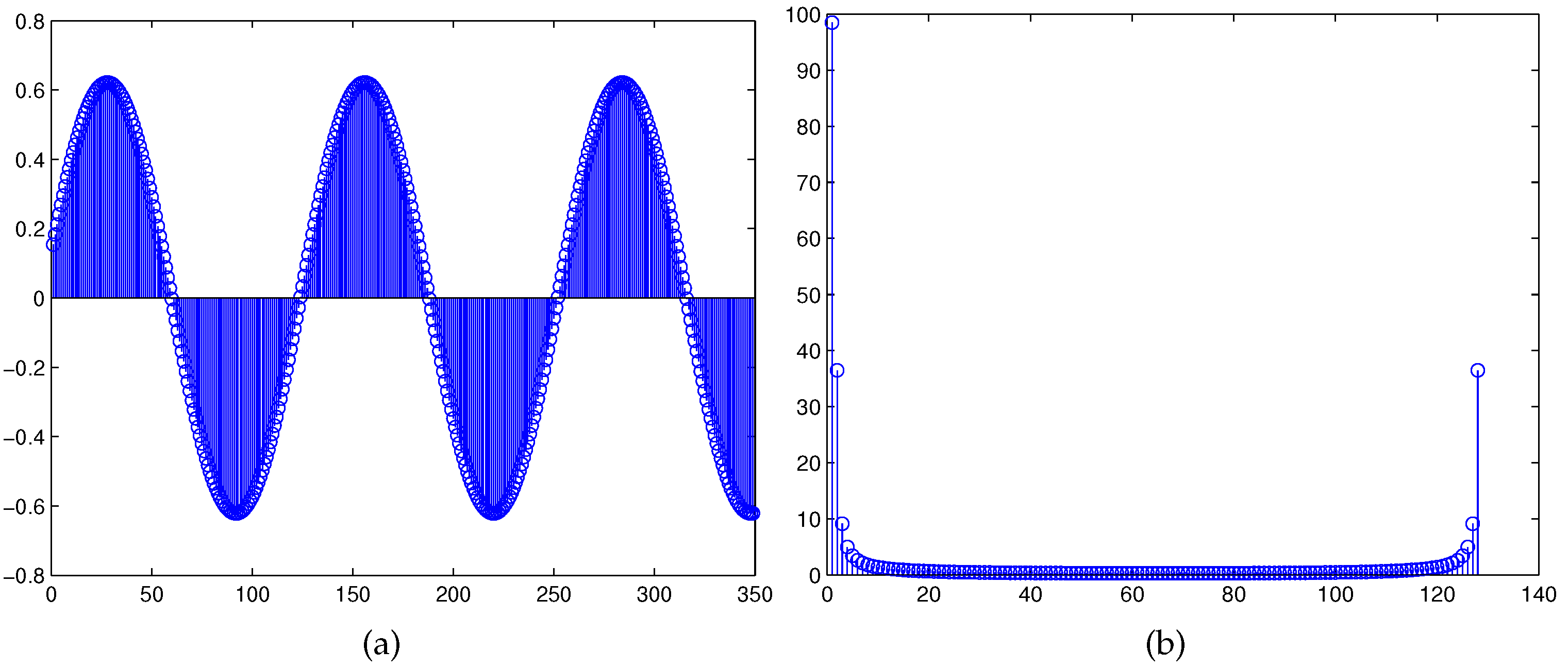
Here, let Hz. The signal is sampled using the sampling rate, Hz. The sampling results are shown in Figure 7a. The figure shows only the result from 0 to 500 points. To clearly show the harmonic of the signal and signal synchronization, we select the cycle length of the discrete signal in (21) to perform its FFT. Note that there are 128 points per cycle length of the discrete signal according to the sampling rate . The FFT results are shown in Figure 7b. It can be observed that there are many harmonics in the spectrum of the original signal; however, after the SRC operation, no harmonics remain in the spectrum of the re-sampling signal. This demonstrates that our proposed method can be used to perform the SRC, improving its effectiveness.
The signal is sampled using the sampling rate . Note that is an integer multiple of . For the frequency estimation, because spectral leak occurs in the re-sampling process, the frequency estimate converges to 50.20066477092068 Hz, when the iterative estimation is run five times. Table 2 shows the results of the FFT for . It is corrected by the SRC before and after each cycle of .
Table 2 shows the extent of the signal spectrum before and after SRC. Before the SRC, many of the sampled values are zero because is an f integer number. It should be obvious that the signal spectrum still contains a small amount of leakage. This behavior is understandable because the process of sampling rate conversion inevitably has some frequency spectrum leakages. Furthermore, the sampling rate is not strictly equal to the integer time frequency of the signal. However, the base and the maximum amplitude of the harmonic wave amplitude ratio is only , showing that frequency spectrum leakage is very small. This level of accuracy could completely satisfy the face harmonic analysis of a signal and could accurately identify harmonics.
4.4. Comparison Results
4.4.1. Frequency Deviation Estimation
To enable the comparison of the accuracy of this method with the accuracies of alternative solutions, the method of iterative frequency estimation by interpolation on Fourier coefficients (IIFC) [28] is applied to perform the experimental evaluation. The authors proposed and analyzed two new frequency estimators that interpolate on the Fourier coefficients of the received signal samples. The estimators were shown to achieve identical asymptotic performances. The frequency of the signal was derived as
where is the index of the bin with the largest magnitude, and is a residual in the interval .
In this experiment, the signal’s amplitude is 1, and the length of the signal is 256. After using (7) and (22) to estimate the signal frequency, the estimated performances of the two methods are evaluated using the concept of channel request block (CRB). We further use the proposed method and the IIFC to perform the frequency estimation, and then the CRBs of the two methods are analyzed for different signal noise ratios (SNR). For each method, the frequency estimation of the signal is performed 1000 times. We present experimental results on the CRB shown in Figure 8. It can be observed that the CRB decreases as the SNR increases for the two frequency evaluated methods. Obviously, the CRB obtained by our method is better than that obtained by the IIFC. This is because our method intercepts the signal to estimate the signal phase deviation that reflects the variation of the signal frequency. Based on the above analysis, the results of this experiment also indicate that the proposed method outperforms the IIFC for frequency deviation estimation.
4.4.2. Sampling Rate Conversion
To enable accuract comparisons for our proposed method, we applied the batch Farrow filter resampling (BFFR) method [20] to perform the experimental evaluation. In [20], the authors presented a design for an arbitrary sample-rate resampling method using the OTHR for radar applications. The signal presented in (19) was selected to perform the SRC using our proposed method and BFFR.
The results obtained by our proposed method are depicted in Figure 7, while Figure 9 depicts the corresponding converted results obtained using BFFR. Figure 9b shows that serious harmonic wave distortion exists, but, due to the sampling rate, there is no synchronization with the frequency of the signal. However, Figure 7b shows no harmonic wave. From the above analysis, it is clear that our proposed method can be applied to perform the SRC, with better performance than BFFR.
5. Conclusions
In this paper, we propose a simple but effective signal frequency correction and sampling rate conversion method based on DFT. We have demonstrated the performance of the proposed method experimentally using a discrete signal with a frequency of Hz. Our method can be easily adapted to any other discrete signal for different frequencies. Sampling rate synchronization is critical for the resampling of any discrete signal for any application due to serious distortions of the discrete signal. The FFR estimation and the modified Farrow filter of our proposed method can effectively solve the sampling rate conversion for any discrete signal.
Acknowledgments
This work was supported in part by the science and technology research projects of Guangxi universities under Grant KY2015YB367, in part by the teaching reform project of Guilin normal college under Grant XJJG201507, in part by GuangXi Youth project 2017KY0942, and in part by the soft science research plan project in henan province 172400410344. The authors would like to thank anonymous reviewers for their comments which help to significantly improve the paper.
Author Contributions
Changjian Zhu and Hong Zhang conceived and designed the experiments, analyzed the data; Hong Zhang performed the experiments, contributed analysis tools; Changjian Zhu wrote the paper.
Conflicts of Interest
No conflict of interest exits in the submission of this manuscript, and manuscript is approved by both authors for publication.
References
- Vaidyanathan, P.P. Generalizations of the sampling theorem: Seven decades after Nyquist. IEEE Trans. Circuits Syst. I Fundam. Theory Appl. 2001, 48, 1094–1109. [Google Scholar] [CrossRef]
- Nyquist, H. Certain topics in telegraph transmission theory. Trans. Am. Inst. Electr. Eng. 1928, 47, 617–644. [Google Scholar] [CrossRef]
- Shannon, C.E. Communications in the presence of noise. Proc. IRE 1949, 37, 10–21. [Google Scholar] [CrossRef]
- Tavares, G.; Tavares, L.; Petrolino, A. An improved feedforward frequency offset estimator. IEEE Trans. Signal Process. 2008, 56, 2155–2160. [Google Scholar] [CrossRef]
- Chen, X.; Li, Y. An islanding detection method for inverter-based distributed generators based on the reactive power disturbance. IEEE Trans. Power Electron. 2016, 31, 3559–3574. [Google Scholar] [CrossRef]
- Gupta, P.; Bhatia, R.S.; Jain, D.K. Active ROCOF Relay for Islanding Detection. IEEE Trans. Power Deliv. 2017, 32, 420–429. [Google Scholar] [CrossRef]
- Narayanan, K.; Siddiqui, S.A.; Fozdar, M. Hybrid islanding detection method and priority-based load shedding for distribution networks in the presence of DG units. IET Gener. Transm. Distrib. 2017, 11, 586–595. [Google Scholar]
- Viterbi, A.J. Principles of Coherent Communication; McGraw-Hill: New York, NY, USA, 1966; Volume 966, pp. 40–42. [Google Scholar]
- Fitz, M.P. Further results in the fast estimation of a single frequency. IEEE Trans. Commun. 1994, 42, 862–864. [Google Scholar] [CrossRef]
- Mengali, U.; Morelli, M. Data-aided frequency estimation for burst digital transmission. IEEE Trans. Commun. 1997, 45, 23–25. [Google Scholar] [CrossRef]
- Kay, S. A fast and accurate single frequency estimator. IEEE Trans. Acoustics Speech Signal Process. 1989, 37, 1987–1990. [Google Scholar] [CrossRef]
- Tretter, S. Estimating the frequency of a noisy sinusoid by linear regression (Corresp.). IEEE Trans. Inf. Theory 1985, 31, 832–835. [Google Scholar] [CrossRef]
- Brown, T.; Wang, M.M. An iterative algorithm for single-frequency estimation. IEEE Trans. Signal Process. 2002, 50, 2671–2682. [Google Scholar] [CrossRef]
- Gedalyahu, K.; Ronen, T.; Eldar Yonina, C. Multichannel sampling of pulse streams at the rate of innovation. IEEE Trans. Signal Process. 2011, 59, 1491–1504. [Google Scholar] [CrossRef]
- Harris, F. Performance and design of Farrow filter used for arbitrary resampling. Proceedings of 13th International Conference on Digital Signal Processing, Santorini, Greece, 2–4 July 1997; Volume 2, pp. 595–599. [Google Scholar]
- Farrow, C.W. A continuously variable digital delay element. In Proceedings of the IEEE International Symposium on Circuits and Systems, Espoo, Finland, 7–9 June 1988; pp. 2641–2645. [Google Scholar]
- Mitra, S.K.; Kuo, Y. Digital Signal Processing: A Computer-Based Approach; McGraw-Hill: New York, NY, USA, 2006; Volume 2. [Google Scholar]
- Blok, M. Farrow structure implementation of fractional delay filter optimal in Chebyshev sense. In Proceedings of the Photonics Applications in Astronomy, Communications, Industry, and High-Energy Physics Experiments IV, Wilga, Poland, 29 May–4 June 2006; p. 61594k. [Google Scholar]
- Wang, T.; Li, C. Sample rate conversion technology in software defined radio. In Proceedings of the IEEE Conference on Electrical and Computer Engineering, CCECE’06, Ottawa, ON, Canada, 7–10 May 2006; pp. 1355–1358. [Google Scholar]
- Horridge, J.P.; Frazer, G.J. Accurate arbitrary resampling with exact delay for radar applications. In Proceedings of the IEEE 2008 International Conference on Radar, Adelaide, Australia, 2–5 September 2008; pp. 123–127. [Google Scholar]
- Blok, M. Fractional delay filter design for sample rate conversion. In Proceedings of the 2012 Federated Conference on IEEE Computer Science and Information Systems (FedCSIS), Wroclaw, Poland, 9–12 September 2012; pp. 701–706. [Google Scholar]
- Andria, G.; Savino, M.; Trotta, A. Windows and interpolation algorithms to improve electrical measurement accuracy. IEEE Trans. Instrum. Meas. 1989, 38, 856–863. [Google Scholar] [CrossRef]
- Rajamani, K.; Yhean-Sen, L.; Farrow, C.W. An efficient algorithm for sample rate conversion from CD to DAT. IEEE Signal Process. Lett. 2000, 7, 288–290. [Google Scholar] [CrossRef]
- Evangelista, G. Design of digital systems for arbitrary sampling rate conversion. Signal Process. 2003, 83, 377–387. [Google Scholar] [CrossRef]
- Psiaki, M.L. Block acquisition of weak GPS signals in a software receiver. In Proceedings of the 14th International Technical Meeting of the Satellite Division of The Institute of Navigation (ION GPS 2001), Salt Lake City, UT, USA, 11–14 September 2001. [Google Scholar]
- Gupta, P.; Bhatia, R.S.; Jain, D.K. Average absolute frequency deviation value based active islanding detection technique. IEEE Trans. Smart Grid 2015, 6, 26–35. [Google Scholar] [CrossRef]
- Rife, D.C.; Boorstyn, R.R. Single tone parameter estimation from discrete-time observations. IEEE Trans. Inf. Theory 1974, 20, 591–598. [Google Scholar] [CrossRef]
- Aboutanios, E.; Mulgrew, B. Iterative frequency estimation by interpolation on Fourier coefficients. IEEE Trans. Signal Process. 2005, 53, 1237–1242. [Google Scholar] [CrossRef]
Figure 1.
Transmission of a signal with frequency deviation.
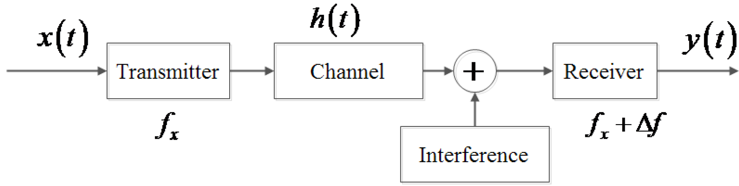
Figure 2.
Diagram of the frequency deviation for a periodic signal.
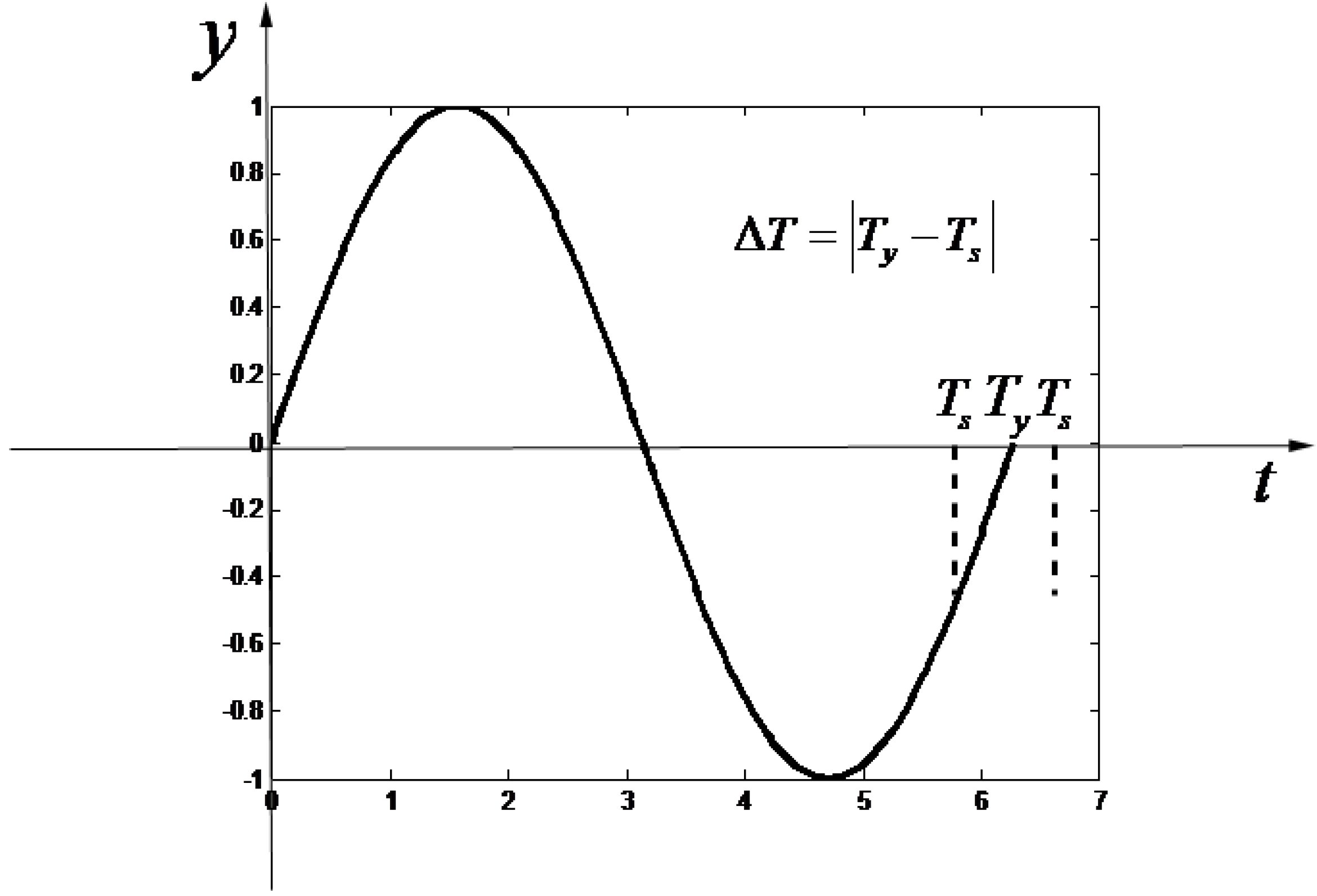
Figure 3.
Subtraction results of interpolation between 2000 points and 10,000 points.
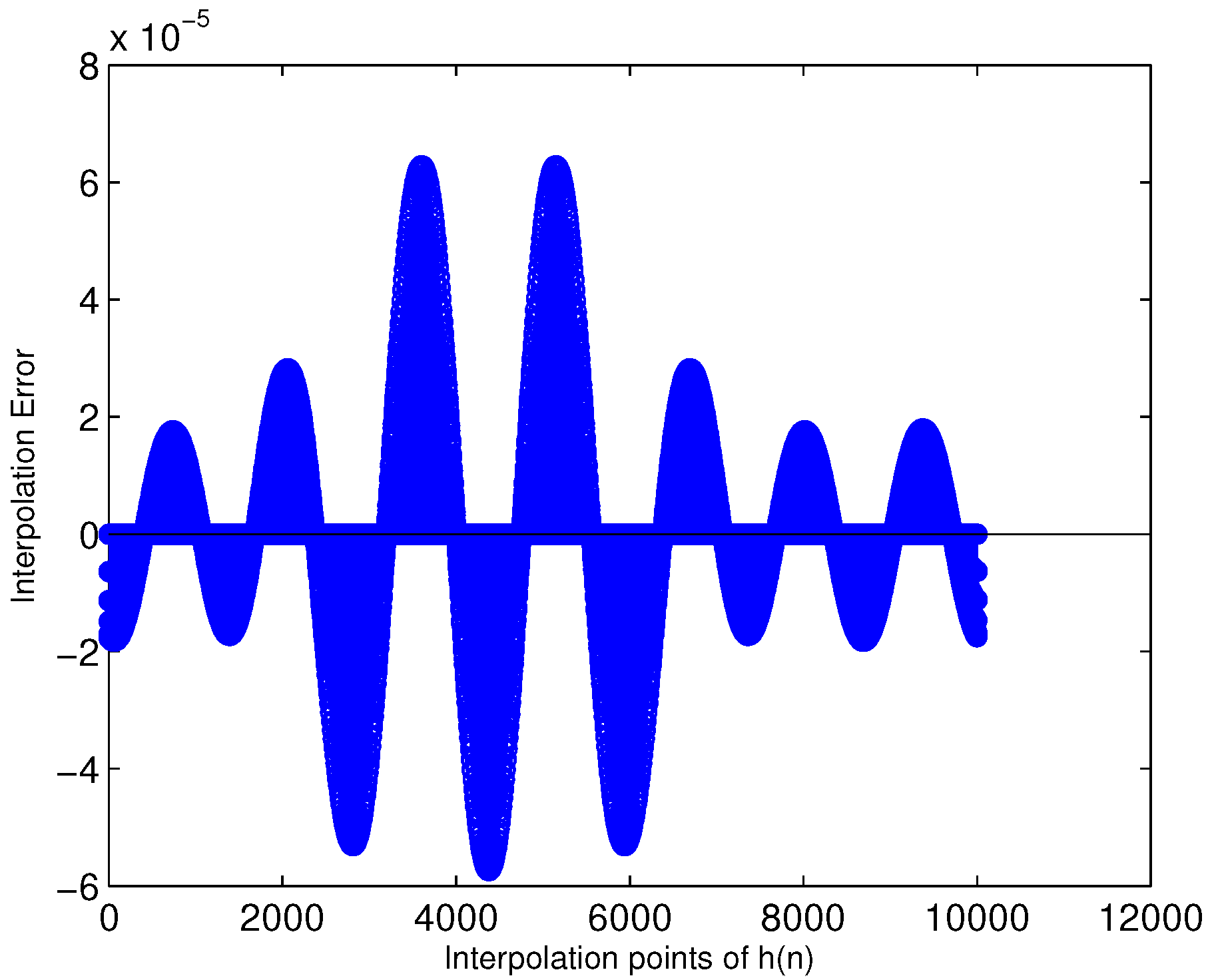
Figure 4.
Diagram of points. The top (a) graph illustrates the interpolation coefficients of , while the bottom (b) illustrates the original coefficients of .
Figure 4.
Diagram of points. The top (a) graph illustrates the interpolation coefficients of , while the bottom (b) illustrates the original coefficients of .

Figure 5.
Diagram of the re-sampling signal. The top (a) graph illustrates the original discrete signal, while the bottom (b) graph illustrates the sampling rate of the converted discrete signal.
Figure 5.
Diagram of the re-sampling signal. The top (a) graph illustrates the original discrete signal, while the bottom (b) graph illustrates the sampling rate of the converted discrete signal.
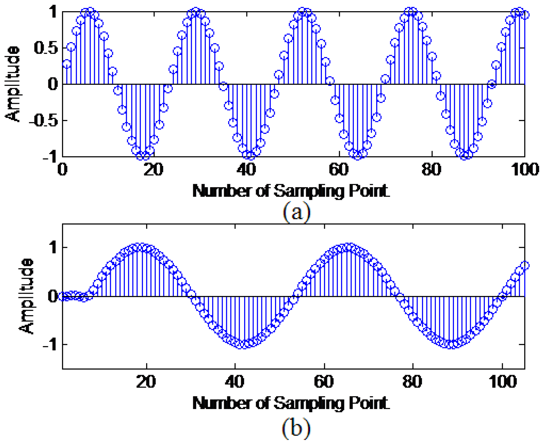
Figure 6.
The spectra of the original discrete signal and the converted discrete signal for the corresponding signal in Figure 5.
Figure 6.
The spectra of the original discrete signal and the converted discrete signal for the corresponding signal in Figure 5.
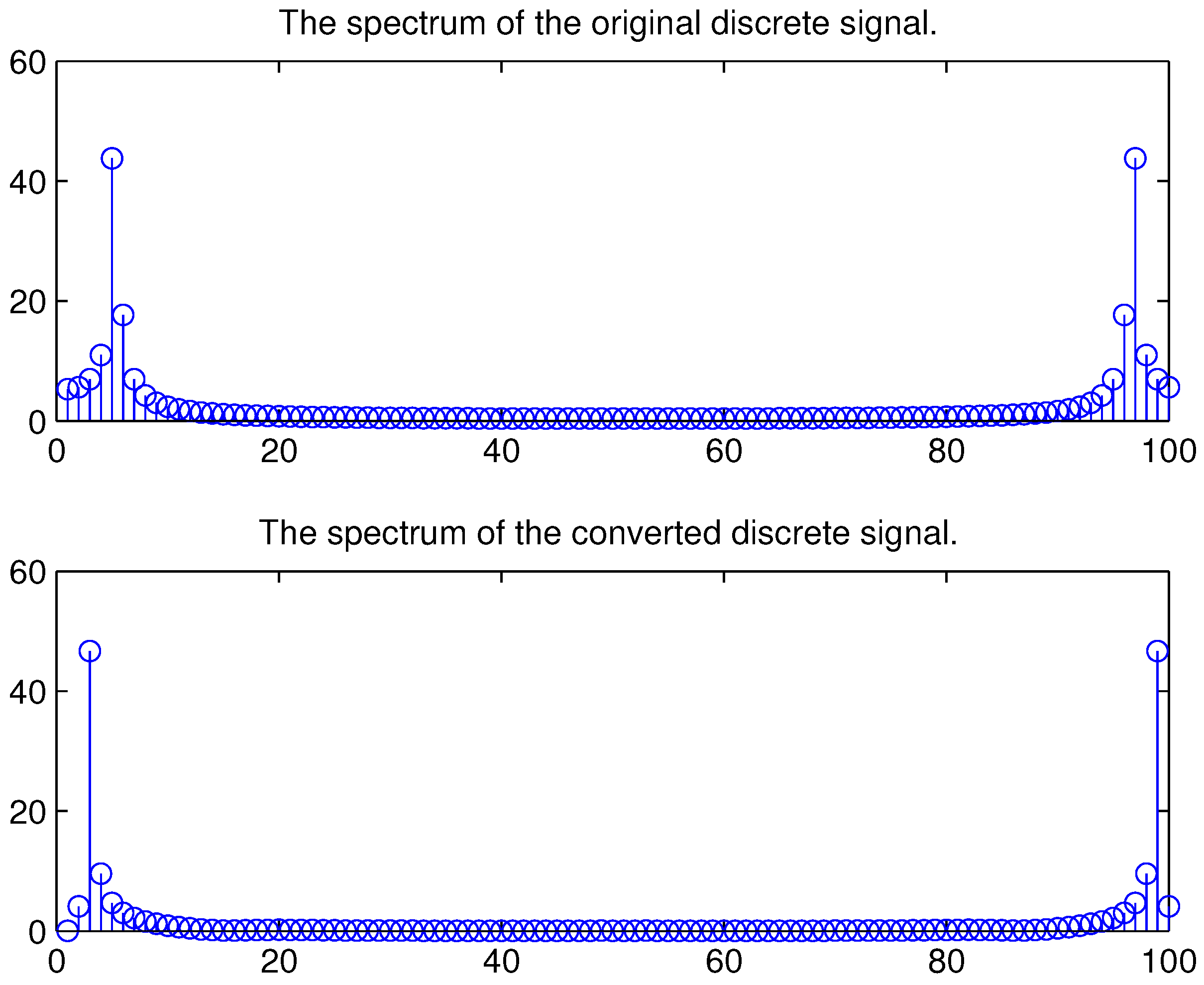
Figure 7.
(a) illustrates the difference between the original signal and the resampled signal for sampling rate synchronization; (b) illustrates the fast Fourier transform (FFT) of the resampled signal for comparison to the original signal.
Figure 7.
(a) illustrates the difference between the original signal and the resampled signal for sampling rate synchronization; (b) illustrates the fast Fourier transform (FFT) of the resampled signal for comparison to the original signal.

Figure 8.
Diagram of the channel request block (CRB) results obtained by our frequency estimation method and by the interpolation on Fourier coefficients (IIFC).
Figure 8.
Diagram of the channel request block (CRB) results obtained by our frequency estimation method and by the interpolation on Fourier coefficients (IIFC).
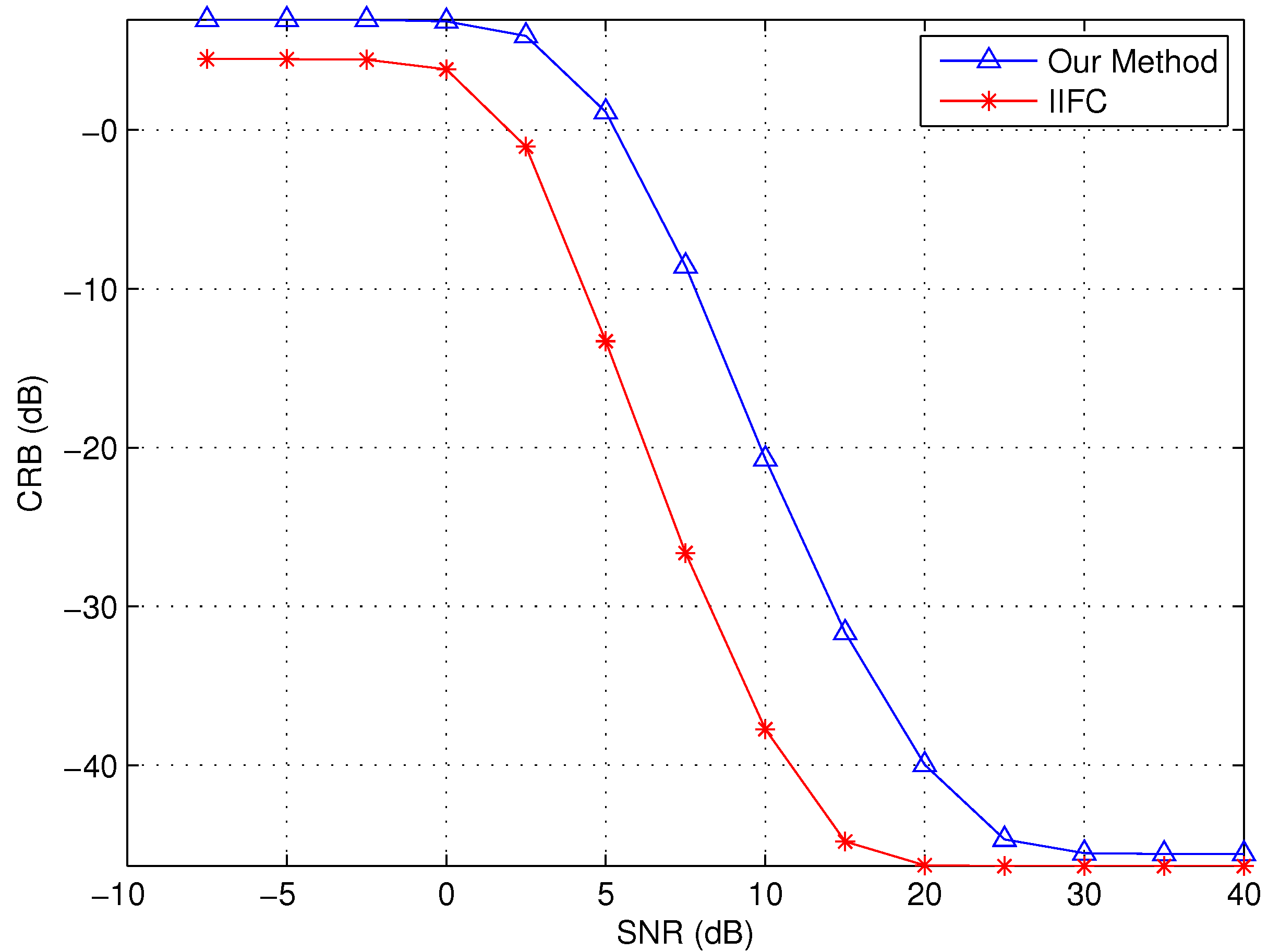
Figure 9.
(a) illustrates the sampling rate conversion after using batch Farrow filter resampling (BFFR); (b) illustrates the spectrum of sampling rate conversion after using BFFR.
Figure 9.
(a) illustrates the sampling rate conversion after using batch Farrow filter resampling (BFFR); (b) illustrates the spectrum of sampling rate conversion after using BFFR.

Table 1.
Simulation results of fine frequency. (Units: Hz.)
| Loop Number | Frequency Estimation | Containing Harmonic | Containing Harmonic and Noise |
|---|---|---|---|
| 1 | 50.200796 | 50.205414 | 50.329538 |
| 2 | 50.20000 | 50.200000 | 50.200333 |
| 3 | 50.20000 | 50.200000 | 50.200000 |
| 4 | 50.20000 | 50.200000 | 50.200000 |
| 5 | 50.20000 | 50.200000 | 50.200000 |
Table 2.
Fast Fourier transform (FFT) comparison of the signals with the theoretical integer sampling rate and the synchronous sampling rate.
Table 2.
Fast Fourier transform (FFT) comparison of the signals with the theoretical integer sampling rate and the synchronous sampling rate.
| The Results of the Sampling Signal for before the sampling rate conversion (SRC) | The Results for after the SRC |
|---|---|
| 0 | 0.00485602103592 |
| 0 | 0.00473329018826 |
| 0.00000000000001 | 0.00435523550826 |
| 0.00000000000001 | 0.00377333106918 |
| 0.00000000000001 | 0.00243896125486 |
| 0.00000000000001 | 0.00038573119211 |
| 0.00000000000001 | 0.00019852719739 |
| 0 | 0.00013465731865 |
| 62.82496056620225 | 62.56533184922048 |
| 20.86262463928692 | 20.77828756114954 |
| 12.42215235579411 | 12.37393682470713 |
| 8.76973611504727 | 8.73749834116767 |
| 0 | 0.00070606042704 |
| 0.00000000000001 | 0.00026219741259 |
| 0 | 0.00016016198162 |
© 2017 by the authors. Licensee MDPI, Basel, Switzerland. This article is an open access article distributed under the terms and conditions of the Creative Commons Attribution (CC BY) license (http://creativecommons.org/licenses/by/4.0/).
Share and Cite
MDPI and ACS Style
Zhang, H.; Zhu, C. A Filter Structure for Arbitrary Re-Sampling Ratio Conversion of a Discrete Signal. Information 2017, 8, 53. https://doi.org/10.3390/info8020053
AMA Style
Zhang H, Zhu C. A Filter Structure for Arbitrary Re-Sampling Ratio Conversion of a Discrete Signal. Information. 2017; 8(2):53. https://doi.org/10.3390/info8020053
Chicago/Turabian StyleZhang, Hong, and Changjian Zhu. 2017. "A Filter Structure for Arbitrary Re-Sampling Ratio Conversion of a Discrete Signal" Information 8, no. 2: 53. https://doi.org/10.3390/info8020053
Note that from the first issue of 2016, this journal uses article numbers instead of page numbers. See further details here.