A Routing Protocol Based on Received Signal Strength for Underwater Wireless Sensor Networks (UWSNs)

1
Department of Computer, Qinghai Normal University, Xining 810008, China
2
Key Laboratory of the Internet of Things of Qinghai Province, Xining 810008, China
3
College of Physics and Electronic Information Engineering, Qinghai Nationalities University, Xining 810007, China
*
Author to whom correspondence should be addressed.
Information 2017, 8(4), 153; https://doi.org/10.3390/info8040153
Submission received: 23 October 2017
/
Revised: 17 November 2017
/
Accepted: 22 November 2017
/
Published: 24 November 2017
Abstract
:Underwater wireless sensor networks (UWSNs) are featured by long propagation delay, limited energy, narrow bandwidth, high BER (Bit Error Rate) and variable topology structure. These features make it very difficult to design a short delay and high energy-efficiency routing protocol for UWSNs. In this paper, a routing protocol independent of location information is proposed based on received signal strength (RSS), which is called RRSS. In RRSS, a sensor node firstly establishes a vector from the node to a sink node; the length of the vector indicates the RSS of the beacon signal (RSSB) from the sink node. A node selects the next-hop along the vector according to RSSB and the RSS of a hello packet (RSSH). The node nearer to the vector has higher priority to be a candidate next-hop. To avoid data packets being delivered to the neighbor nodes in a void area, a void-avoiding algorithm is introduced. In addition, residual energy is considered when selecting the next-hop. Meanwhile, we establish mathematic models to analyze the robustness and energy efficiency of RRSS. Lastly, we conduct extensive simulations, and the simulation results show RRSS can save energy consumption and decrease end-to-end delay.
1. Introduction
In the last few decades, more and more researchers have been attracted to UWSNs (underwater wireless sensor networks). UWSNs have prospective applications in resource exploitation, disaster detection, aided navigation, and so on. UWSNs are different from terrestrial wireless sensor networks, and have many inherent features [1]. RF (radio frequency) signal is unsuitable for use in the UWSNs because of obvious attenuation; optical signals cannot be used owing to the multipath and Doppler effects either. Therefore, UWSNs use acoustic waves to communicate [2].
To design a communication system, we have to consider these features in UWSNs [3]: (1) low available bandwidth; in UWSNs, the available bandwidth is less than 100 KHz; (2) dynamic topology; the underwater sensor nodes usually move with water current, which leads to the uncertainty of neighbor nodes and varied topology; (3) limited energy; underwater sensor nodes are powered by batteries which are hard to replace or recharge. Once the power runs out, the sensor node is considered to be dead [4]; (4) unknown position; positioning technology used on land, such as GPS, is not applicable in UWSNs.
For all the above, routing protocols used in terrestrial sensor networks cannot be directly used in UWSNs. So, designing routing protocols tailored for UWSNs is necessary [5], and scholars have proposed some routing protocols for UWSNs which are applied to certain scenarios. However, these protocols have some defects, which are detailed in Section 2.
In this paper, in order to decrease energy consumption and shorten delay, we propose a routing protocol for UWSNs based on received signal strength (RRSS). In RRSS, each node maintains a vector from itself to a sink node. After receiving a data packet, the receiving node selects the neighbor nearest to the RSS vector as the best next-hop. In our protocol, there are two kinds of control messages. One is the control message from a sink node, which is called a beacon message, and another is a “hello” message from a neighbor sensor node. The RSS of a hello packet (RSSH) indicates the distance from itself to its neighbor as well as the link quality. The RSS of the beacon signal (RSSB) is used to reflect the link quality and the distance to the sink node. Candidate next-hop nodes are those neighbor nodes with stronger RSSB. When the RSSB of neighbor nodes is the same, the sender determines the priority of the neighbor nodes according to RSSH: the stronger RSSH, the higher priority to be the next-hop. However, data packets may be delivered to a node in a void area or without enough residual energy. Therefore, we introduce a residual energy threshold as well as a void-avoiding algorithm when selecting the best next-hop node.
Our contributions are summarized as follows:
- We provide a method to construct the vector with the least energy consumption from the source node to a sink node independent of location information, and this is suitable for networks with both a single sink node and multiple sink nodes.
- We propose RSS as the parameter to select next-hop. RSS can not only reflect propagation distance but also noise power, which decreases delay and saves on energy consumption.
- We consider void node and energy threshold in our protocol to avoid data packets being delivered to the nodes in a void area or without sufficient residual energy.
- We establish mathematical models to analyze the energy-efficiency and robustness of RRSS.
The paper is organized as follows: In Section 2, we introduce related work. In Section 3, we describe the RRSS routing protocol. In Section 4, we build a mathematical model to analyze the performance of RRSS. In Section 5, we conduct extensive simulations and evaluate the performance of RRSS. Section 6 concludes the paper.
2. Related Works
As mentioned before, UWSNs are different from WSNs on land. Many routing protocols used in WSNs are either inapplicable, or have low efficiency in UWSNs. Recently, some researchers have been designing routing protocols to support the application of UWSNs.
In vector based forwarding (VBF) [6], the sensor nodes need not acquire the state information. From the source node to the destination node, VBF constructs a pipe using a vector. The nodes in the pipe may be selected as the forwarding nodes; the nodes outside the pipe do not participate in forwarding. However, VBF is a location-based routing approach. It needs information on the location of all the nodes, which is another problem. According to the pressure of sensor nodes under water, in [7,8,9] the authors proposed routing protocols based on pressure. Yan et al. proposed depth-based routing (DBR) in [10], which needs only local depth information. To acquire the depth, each underwater sensor is equipped with a pressure sensor. After receiving a packet, the sensor node judges whether it is a candidate as forwarding node by the difference between its depth and the sender’s. Maybe there are many candidate nodes; so, to avoid all the qualified nodes forwarding packets redundantly, a technique of suppressing redundant forwarding is introduced in DBR. The location information of nodes is not necessary in DBR.
However, DBR has some defects; for example, link quality and residual energy are not considered, and essential redundant forwarding in DBR leads to considerable energy consumption. Therefore, many improved protocols have been proposed based on DBR. EEDBR considers the depth and residual energy in [11]. Due to the complex underwater environment, considering only residual energy is not enough. The depth-controlled routing (DCR) protocol was proposed in [12]. In DCR, the underwater sensor nodes are equipped with network topology controllers, which are used to adjust their depth when the greedy geographic routing fails. Clearly, DCR is a geographical routing protocol, and it requires geographical location information in order to control the topology structure, which is so far an unsolved problem. In [13], Tairq proposed the L2-ABF protocol. In L2-ABF, the underwater 3D-space is divided into layers. To save energy and decrease redundant forwarding, a node first calculates its flooding angle. The underwater sensor nodes forward data only to the nodes in the shallower layers. If a node fails to find a qualified next-hop after broadcasting a control packet at initial power and angle, then it increases the transmitting power as well as the broadcasting angle. L2-ABF is a location-based routing protocol. However, it does not provide a specific scheme to determine the initial flood angle. After all, the initial angle is related to node density. In addition, the priority of receiver is set according to the residual energy threshold, which leads to redundant forwarding. In [14], the link expiration time-aware routing protocol (LETA) was proposed. In LETA, the priority of candidate nodes is calculated based on the Bayes theory, in which the depth, residual energy and distance are used as the parameters for calculating forwarding probability. However, LETA needs to acquire location information, and to calculate new location when nodes are mobile, which is complex and energy intensive. The channel-aware routing protocol (CARP) was presented in [15], which is location-free. In CARP, the depth is considered as well as the link quality. The node broadcasts a “ping” packet to search a route, which consumes a lot of energy. To improve the energy efficiency, Zhang et al. proposed E-CARP [16]. In E-CARP, the most recently used node is preferentially selected as the next-hop. Due to the dynamic topology, the most recently used node may be not the best next-hop. The directional flooding-based routing protocol (DFR) was proposed in [17]. DFR increases the directional angle in flooding. The number of nodes participating in forwarding is determined by the flooding angle. DFR can prevent flooding effectively to the whole network. However, it has an impractical assumption that all nodes know their geographic location. In [18], Du et al. proposed LB-AGR, which defines an integrated forwarding factor for each candidate node based on available energy, density, location, and level-difference between neighbor nodes, and is used to determine the best next-hop among multiple qualified candidates. The adaptive mobile of courier nodes in threshold-optimized DBR protocol (AMCTD) was proposed in [19]. AMCTD uses adaptive depth threshold, which solves different depth thresholds in networks with different density nodes. The energy-consumption of the upper nodes is decreased by the courier nodes’ movement. However, the movement of courier nodes makes AMCTD unsuitable for data-sensitive applications during the instability phase. So Javaid et al. proposed i-AMCTD in [20]. i-AMCTD precedes AMCTD by introducing both hard and soft thresholds. In addition to sending a hello packet, it sends threshold data. However, sending a threshold consumes a lot of energy. In [21], the authors proposed a routing protocol based on the transmission time. The neighbor with the least transmission time to the sender has the highest priority. Although the route leads to less delay, the link quality and energy-consumption are not considered.
3. RRSS Protocol
3.1. Motivation
Decreasing energy-consumption is a major objective for designing protocols for UWSNs. On the one hand, the energy of sensor nodes underwater is limited. Nodes are powered by batteries, which are hard to recharge and replace. On the other hand, an acoustic signal consumes more energy than a radio signal during communication.
Shortening the delay is another major objective in UWSNs. The propagation speed of acoustic signals underwater is 1500 m/s, which is five orders of magnitude lower than the speed of RF signals in the air, so the propagation delay is the main part of system delay in UWSNs. Therefore, shortening the propagation distance in the path from source node to destination node is an effective way to decrease system delay [22]. The propagation distance affects directly the signal attenuation. The relation between propagation distance and attenuation is shown as Equation (1).
Here, is the unit-normalizing constant; is path loss or attenuation over distance when communication frequency is ; is constant 1.5 for a practical scenario [17]. From Equation (1) we can see that the signal attenuation increases with increasing of communication distance. So, shortening the propagation distance can decrease energy consumption. Therefore, the path with the least energy consumption is the path with the least propagation distance.
In addition, the underwater environment is harsh, and communication quality is affected by diversified noises, including waves, shipping, wind and thermal noises [23]. Among all the routing protocols proposed, DBR and VBF are the most popular. Both are greedy broadcasting routing protocols. VBF is based on location information, which is another unsolved problem. DBR is half independent on geographical location information. However, because of the nature of broadcasting in a densely distributed network, DBR consumes a lot of energy.
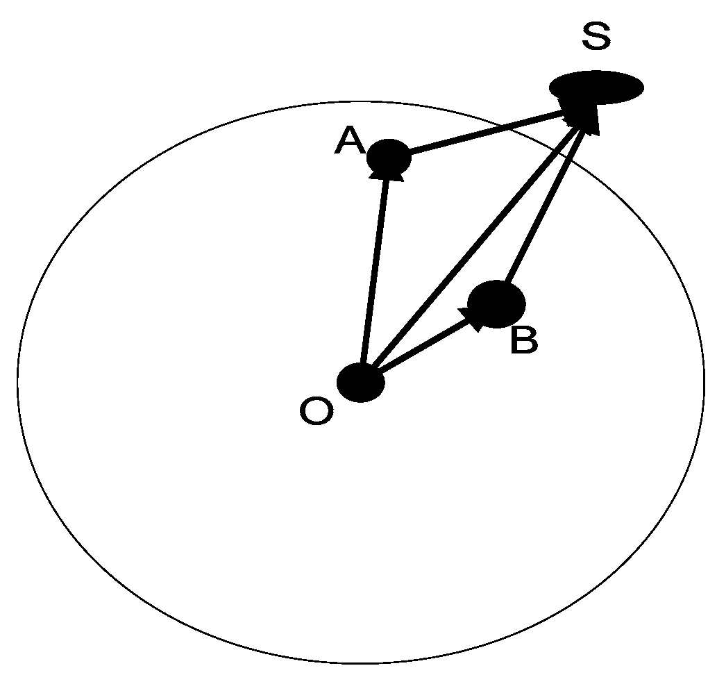
For example, in Figure 1, there is only one sink node S on the water surface, and the data packet from node A can be delivered by two paths. The path 1 is . The path 2 is . Node A, B and S are on a straight line. According to triangle relation, , clearly, the propagation distance of path 2 is shorter than path 1. However, according to DBR, path 1 should be selected as the forwarding path, which consumes more energy and increases delay clearly.
To solve the problems in VBF and DBR as mentioned above, a routing protocol with higher energy efficiency, shorter delay and independent of locations should be proposed for UWSNs.
In our algorithm, each node firstly establishes a vector from itself to a sink node according to RSSB. The RSS depends on the transmission power, the attenuation of the signal, and link quality. RSS can be calculated by Equation (2). The attenuation is related to the propagation distance, which can be seen in Equations (3)–(5). Link quality is reflected by the noise power, as in Equation (6). Therefore, RSS can reflect the propagation delay, energy consumption and link quality of the path. So, RSS is used as the main parameter for selecting the best next-hop in the RRSS routing protocol. The realization of our protocol is simple and suitable for the networks with both single sink node and multiple sink nodes.
Combining Equation (1), we get Equation (5):
In Equation (5), represents the transmitting power of the sender; denotes the receiving power; represents the power amplification, which is denoted by Equation (4); is the maximum instantaneous value; is the minimum instantaneous value of the received signal strength index, which is measured within a given period of time, and node-transmitting maximum power , and minimum power , within a given period of time. When , [24]. In Equation (6), the presents noise power spectral density in [23]; denotes the maximum signal frequency; and denotes the minimum signal frequency.
3.2. Network Structure
As in Figure 2, in this paper sensor nodes are deployed in a 3D space. Sink nodes are distributed evenly on the water surface. Each sink node is equipped with both a radio modem and acoustic modem. Underwater sensor nodes are deployed underwater randomly and equipped with an acoustic modem. Acoustic modems are used to transmit acoustic signals between underwater nodes. Radio modems are used to transmit RF signal between sink nodes and the data center. Each sensor node is equipped with a timer and an instrument for measuring RSS. All underwater sensor nodes can generate and relay data packets. Underwater sensor nodes are mobile in the horizontal direction with water current; the vertical movement can be negligible. In RRSS, we assume the energy of sink nodes is unlimited. This assumption is reasonable because sink nodes can be charged by solar energy. For underwater sensor nodes, once the energy runs out, the node will die. Meanwhile, we assume sink nodes can transmit at enough power to cover the whole area of interest. The transmitting power of underwater sensor nodes is either the same or smaller than sink nodes. We consider the delivery is successful when data packets are received by any one of the sink nodes.
3.3. RRSS Scheme
Here, a few of terms are explained as following.
- Void node: The RSSB of a void node is stronger than that of its neighbors, but all the sink nodes are outside of its transmission range.
- RSS vector: The straight line from an underwater node to a sink node is called a RSS vector. It reflects the routing path with the least attenuation and noise from the node to the sink node.
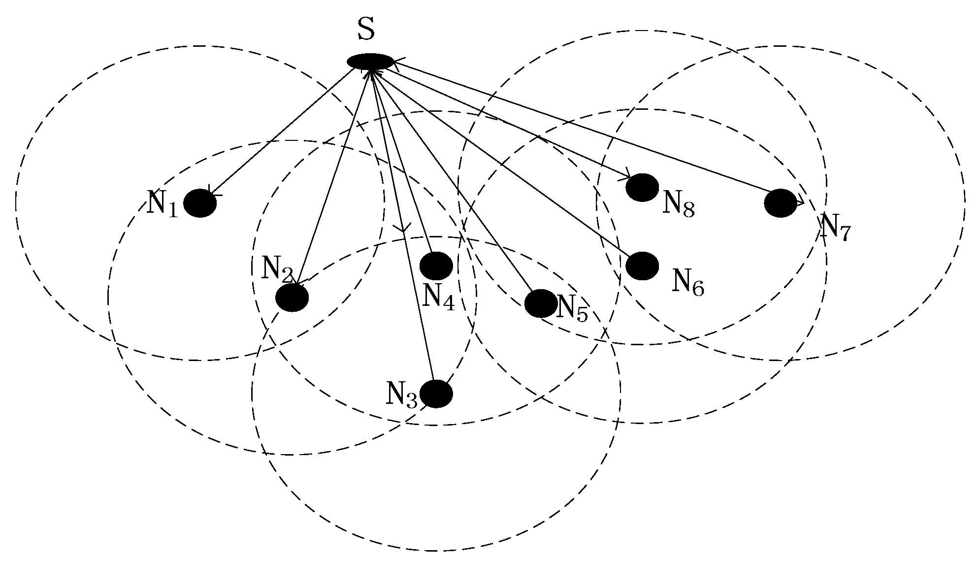
As in Figure 3, nodes N2, N3 and N5 are the neighbors of node N4. The RSSB received by node N4 is stronger than nodes N2, N3 and N5. So, node N4 is a void node. The straight line from one sensor node to the sink node S is the RSS vector of data transmission; for example , and so on.
In RRSS, we divide the underwater nodes into different levels according to the RSSB. The nodes in the same level, we consider to have the same RSSB. A sender selects the next-hop firstly according to the RSSB saved in the candidate routing table; the neighbor with the strongest RSSB has the highest priority. When the RSSB is the same, the node with stronger RSSH has higher priority. The node with less residual energy than the energy threshold does not send a hello packet, because these nodes are not qualified to be forwarding nodes. To avoid data packets being delivered into a void node, the sender selects the neighbor whose void field is 0 as the next-hop.
As in Figure 4, the underwater sensor nodes are classified into three types according to RSSB: SSSN, ESSN and BSSN. The nodes with the same RSSB are called equal signal strength nodes (ESSN). BSSN represents the neighbor nodes with bigger RSSB than that of ESSN. SSSN denotes the neighbor nodes with smaller RSSB than that of ESSN.
RRSS includes three phases. The first phase is initialization. In this phase, each sink node broadcasts beacon messages periodically at enough power, and each node in the area of interest can hear the beacon messages. After receiving the beacon messages, the sensor node records the RSSB and constructs a RSS vector to a sink node. Then, the node broadcasts hello packets periodically.
In the second phase, each underwater node finds the candidate next-hops along the RSS vector. When a node receives a hello packet from a neighbor node, it checks the information of the residual energy and RSSB of the neighbor in the packet. If the residual energy and RSSB of the neighbor meet the given conditions, the neighbor becomes a candidate next-hop node.
The third phase is finding the best next-hop. According to the information of candidate nodes, the priority of the candidates for next-hop is calculated. The sender selects the candidate nearest to the RSS vector as the best next-hop node. A detailed computation process of the priority is provided in Section 4.3.
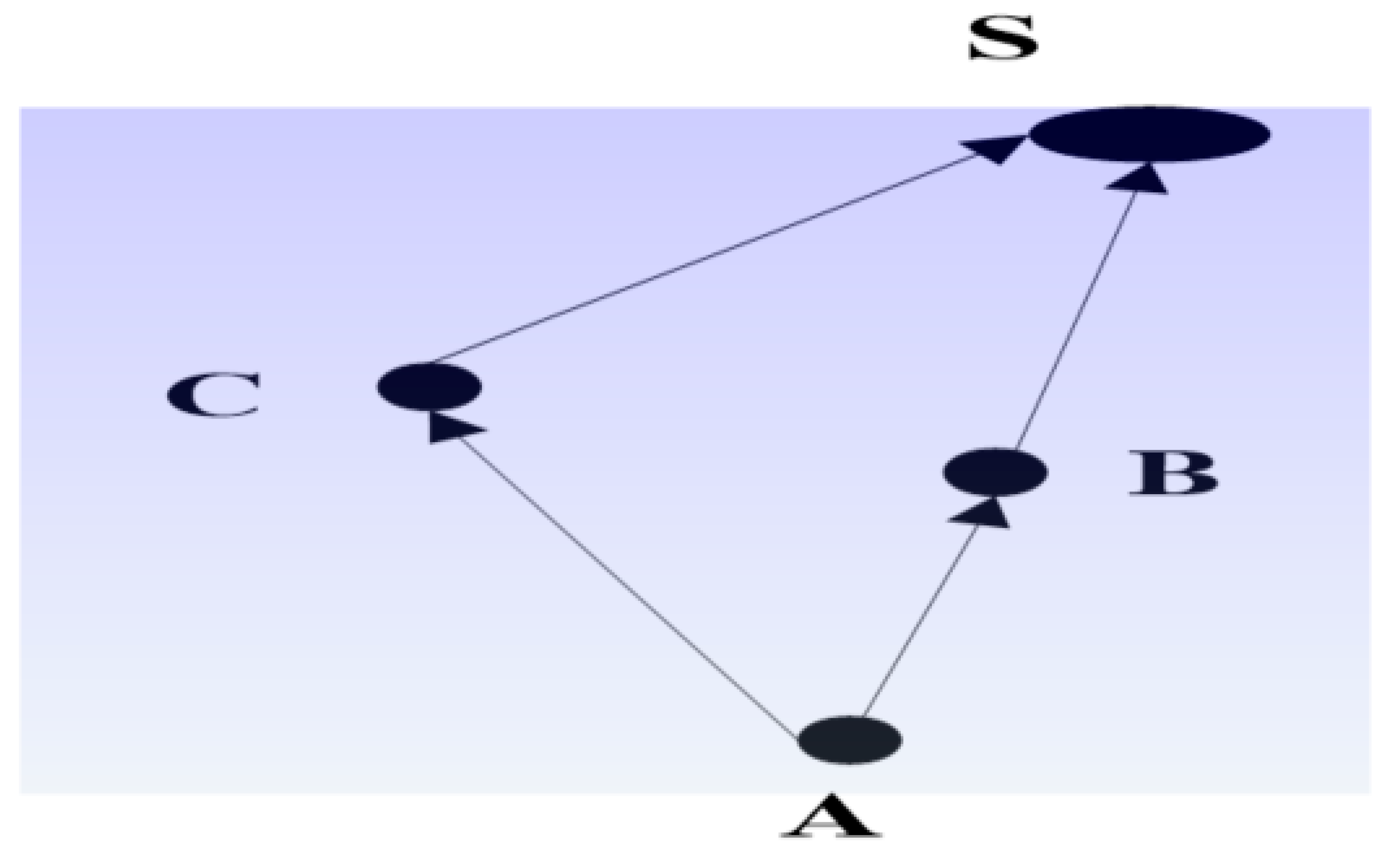
According to Equations (2)–(6), to get closer to the sink node, the neighbors with bigger RSSB than the sender are eligible to be the candidate forwarding nodes. However, the neighbor node with the biggest RSSB may not be the neighbor nearest to the RSS vector. From Figure 5, we can see node A is the nearest to the sink node S, but the node nearest to the vector is node B in the neighbors of node O. So, in RRSS, the priorities of neighbor nodes are calculated combining RSSH and RSSB.
Lemma 1.
If candidate nodes are ESSNs, then the candidate with stronger RSSH has higher priority.
Proof.
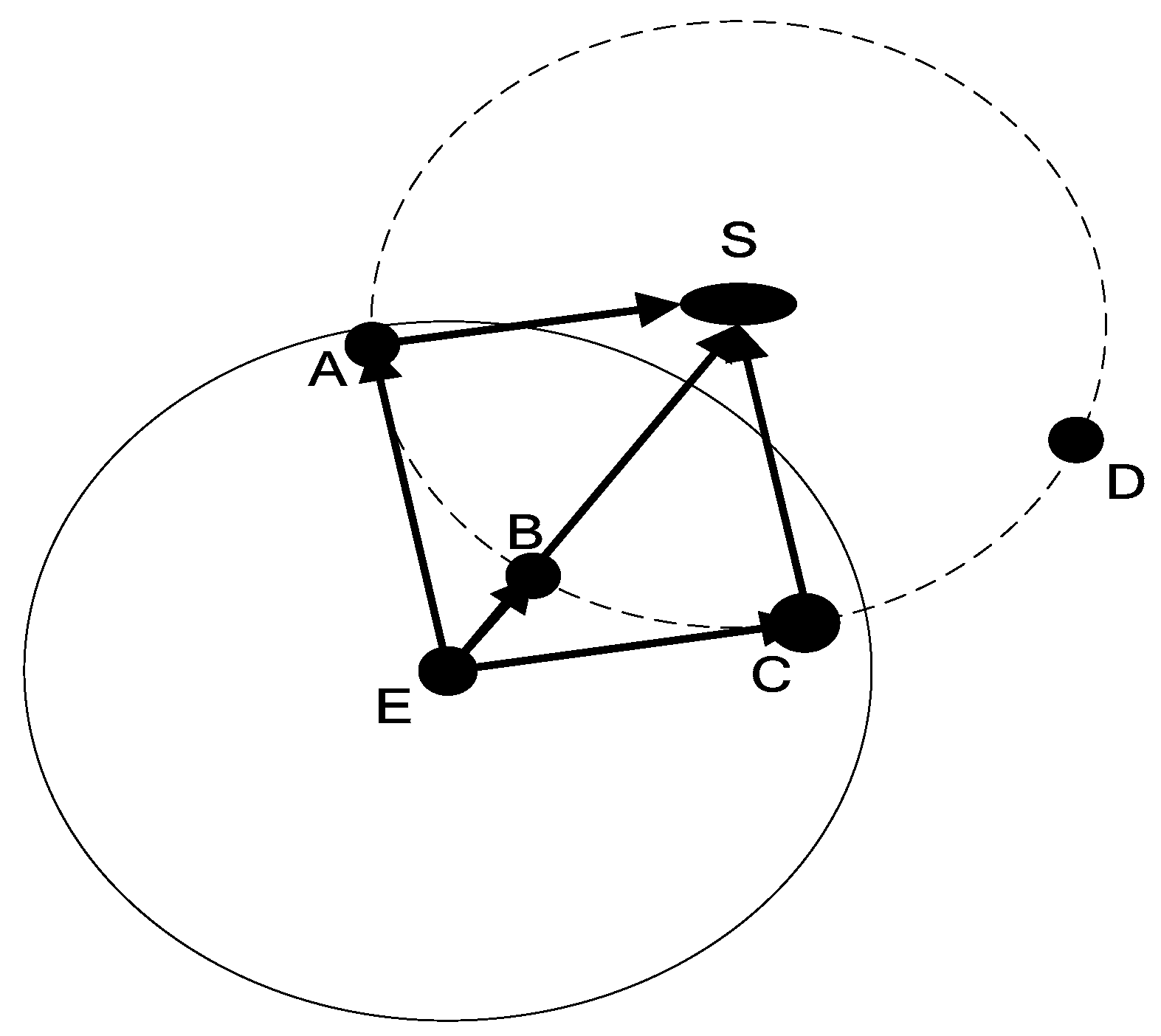
In Figure 6, nodes A, B, C, D are ESSNs. Node B is on the RSS vector. Nodes A, B and C are neighbors of node E. Node E is the sender. According to the RRSS mentioned before, nodes A, B and C are eligible candidate-forwarding nodes. Clearly, the path through node B leads to shorter delay and less noise. In order to determine the best next-hop, node E compares the RSSH from ESSNs, and the candidate with stronger RSSH has higher priority. ☐
For simplicity, this paper considers the situation in which there is only one sink node although RRSS is suitable for both networks with one sink node and multiple sink nodes. When there is more than one sink node on the surface, a sensor node can receive beacon signals from different sink nodes; the node temporarily selects the sink node with the strongest RSSB as the destination.
Each sensor node can receive hello packets from its neighbors, and the sender determines the candidate next-hop nodes according to the information in the hello packets.
The hello packet consists of five fields as follows:
Source node ID: Node ID of the node generating the hello packet.
Beacon Source ID: The source node ID of the beacon signal with the strongest RSSB received by the source node of hello packet.
Beacon Seqno: Beacon signal sequence number of the strongest RSSB received by the source node of hello packet.
Void: Whether the source node of the hello packet is in the void area or not. If the node is in a void area, the “void” field is filled with “1”, which indicates the node is eligible for the candidate next-hop node; otherwise the field is filled with “0”, which indicates the node isn’t eligible for the candidate next-hop node.
RSSB: The receive signal strength of the beacon signal received by the source node of hello packet.
The candidate next-hop table consists of four fields as follows:
Candidate Node ID: Node ID satisfying the condition of the next-hop forwarding node.
Beacon Source ID: The source node ID of the strongest RSSB received by the candidate node.
Beacon Seqno: The sequence number of the beacon signal with strongest RSSB received by the candidate.
Priority: The priority of the candidate next-hop node, which is determined by the suppressing factor. The detailed calculation process of suppressing factor is shown in Section 4.3.
3.3.1. Residual Energy
In RRSS, sensor nodes on the bottom only generate data packets and hello packets. The other nodes can forward data packets as well as generate packets. Compared with the nodes in receiving and idle status, the node in sending status consumes more energy, so the energy consumption in receiving and idle status is neglected in our paper.
For sensor nodes on the bottom, the residual energy can be calculated as Equation (7).
Here, denotes the initial energy of underwater nodes; and represent the number of data packets and hello packets generated respectively; and and represent the energy consumption of sending one data packet and one hello packet respectively. For those underwater sensor nodes which are not on the bottom, the residual energy can be calculated as Equation (8)
Here, represents the number of forwarding data packets; and represents the energy consumption of forwarding one data packet. Comparing Equation (7) with Equation (8), we can see the shallower the node is, the shorter the node lives.
In RRSS, to avoid data packets being delivered to the nodes without enough energy, an energy threshold is set in advance. Only nodes with residual energy greater than the energy threshold are qualified to be candidate next-hop nodes.
3.3.2. Void-Avoiding Algorithm
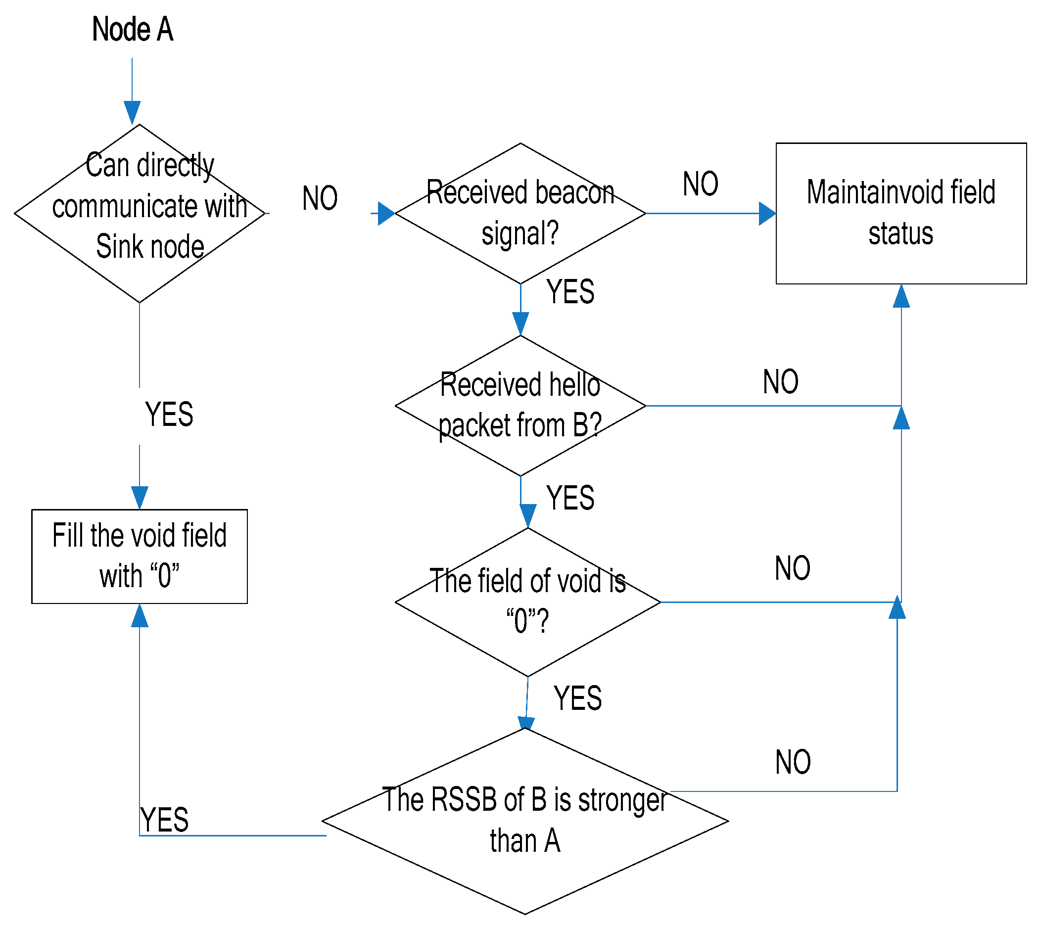
In the initialization phase, each sensor node broadcasts a hello packet periodically, and a “void’’ field is included in the hello packet to denote whether it is a void node or not. The procedure of void-avoiding algorithm is showed in Figure 7. Firstly, the sensor node which is unable to communicate directly with sink nodes fills the void field with “1” in its hello packet before receiving any hello packet from others, then broadcasts the hello packet periodically. The nodes which can communicate directly with the sink node fill the void field with “0”. After receiving a hello packet with a stronger RSSB and “0” void field from a neighbor, the node fills the void field with “0” in its hello packet. After receiving a new beacon signal from the sink nodes, the node updates the beacon seqno in the candidate routing table and initiates the void node field with “1” in its hello packet. When a new hello packet is received, the node updates the void field according to the RSSB and void field of its hello packet according to the RSSB and void field in the hello packet from neighbors. A hello packet with a void node field filled with “0” indicates the neighbor is not a void node.
When a node receives a hello packet of the void field filled with “0”, the source node of the hello packet is qualified to be the candidate next-hop node. However, when the void field fills with “1”, the source node of hello packet is not qualified to be the candidate next-hop.
4. Mathematical Analysis
4.1. Robustness
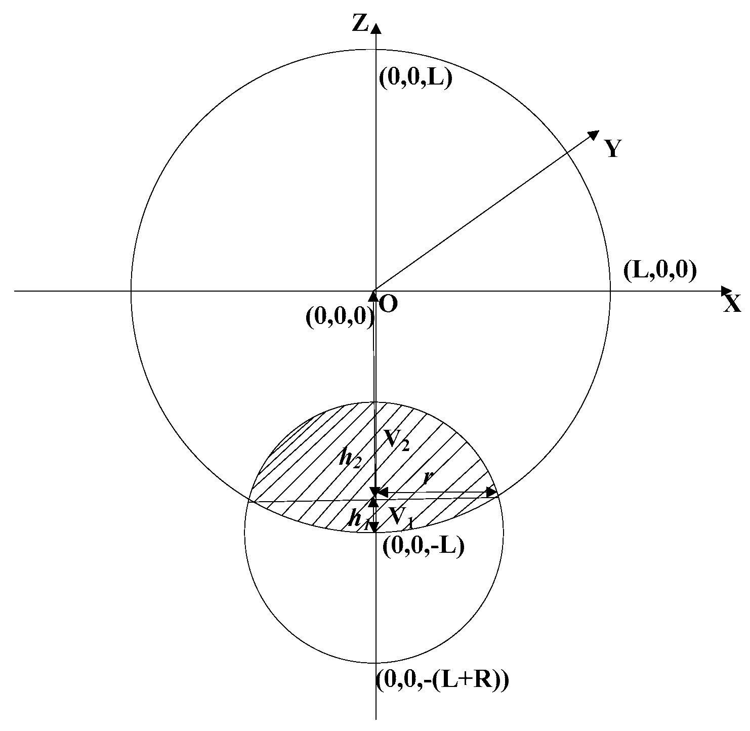
In RRSS, after sending a data packet to the best next-hop, the sender waits for a reply message from the receiver. If the receiver fails to forward the data packet, it will not send the reply packet. If the sender does not receive the reply message, it will delete the routing, then select the best next-hop among the candidates again. When all the candidate nodes fail to send reply messages, we think the delivery fails. We assume the density of nodes is (the number of nodes per square meter). The volume of the candidate area is related to the communication range of the sender and the distance from the sender to the sink node. In order to facilitate analysis, we put the area of interest into a 3D coordinate system.
As in Figure 8, the coordinate of the sink node is (0, 0, 0), and the coordinate of the sender is (0, 0, −L). Candidate nodes are in the shaded part; the number of candidate nodes is N. The volume of the shaded part can be divided into two parts, and . and are the height of two ball-lackings. Then we obtain Equation (9).
Here, the parameters in Equation (9) meet Equation (10).
The variable can be obtained from Equation (11).
From Equations (11) and (12), we get , , . Putting and into Equation (9), we get the number of candidate nodes as Equation (13).
The relationship between the volume of the candidate area and the distance from the sender to the sink node is shown in Figure 9. From Figure 9 and Equation (13), we can see that the number of candidate-forwarding nodes increases with the increase in the distance from the sender to the sink node. If we assume the probability of successful delivery to one of the candidate nodes is p, and the number of candidate nodes is , then the probability of successful deliver to the next-hop is .
The average distance from the sender to the next-hop node is l. The distance from the source node to the sink node is denoted by . The hop number from source to sink is . denotes the number of candidate nodes at the hop. Therefore, the probability of a data packet being successfully delivered to a sink node is P.
4.2. Energy-Consumption Analysis
Here, we call the nodes which can directly communicate with sink nodes as the first-hop nodes. The nodes that can directly communicate with the first-hop node are named the second-hop nodes, and so on. We assume the average number of data packets generated by a node is , and the number of data packets generated by nodes in the ith-hop, , is as in Equation (16). indicates the volume of the candidate area from the ith hop to the next-hop.
When using broadcast routing, such as VBF and DBR, the number of nodes involved in forwarding in the ith hop is . Each candidate next-hop forwards a data packet with probability p, and the energy consumption of delivering a data packet from the ith hop to a sink node is . In the same way, we can get Equation (17).
The number of nodes forwarding the data packets from the ith hop to a sink node is:
Equation (17) denotes the total energy consumption of a data packet from the ith hop to the sink node when the priority is not set.
Even if the candidate area is limited, we can see that the number of forwarding nodes is large in a dense network, which wastes limited energy. So, in RRSS we employ unicast routing, and set a priority for each candidate next-hop. In each hop, only the node with the highest priority forwards the data packet.
After setting the priority, the energy consumption of a data packet from the ith hop to a sink node is as in Equation (18):
4.3. Priority Analysis
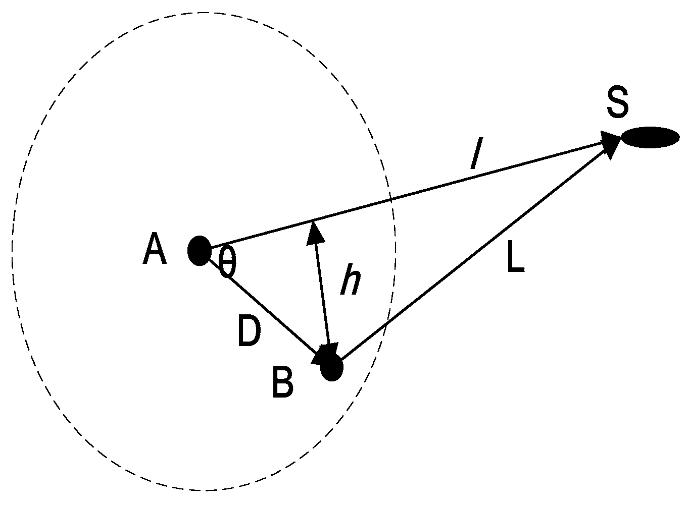
RRSS is a unicast routing protocol; if the node with the highest priority fails to forward the packet, the node with the lower priority has the chance to forward the data packet. The priority is related to the suppressing factor ; the lower suppressing factor, the higher priority. In topology 6, as in Figure 10, D denotes the distance from the sender (node A) to the receiver (node B). represents the distance from the receiver to the sink node (node S); and l denotes the RSS vector. The suppressing factor can be calculated as in Equation (19). Here, h is the distance from the receiving node B to RSS vector.
For clarity, let , according to the Qinjiushao–Helen formula, the area of the triangle ABS, denoted by A, can be calculated as in Equation (20).
The can be calculated as in Equation (22).
When the neighbor is on the RSS vector and the communication radius, the suppressing factor is 0, and the node is considered to be an ideal next-hop. The nearer to 0 the suppressing factor is, the closer to the ideal next-hop the candidate node is. Therefore, we use the suppressing factor as a measure of priority; the lower the suppressing factor, the higher the priority.
5. Performance Evaluation
In this section, we evaluate the performance of RRSS and compare it with DBR and VBF.
5.1. Simulation Settings
Our simulations were conducted using NS2, which includes an underwater sensor network simulation package. The simulation area is a 3-D area of 500 m × 500 m × 500 m. Multiple sinks are deployed on the water surface. The sink nodes are stationary during the simulation procedure. Each sensor node randomly selects a direction and moves to a new position with a random speed between 1 m/s and 5 m/s. The source node is randomly deployed. The broadcast media access control protocol is used as the protocol of the data link layer. The traffic is generated by constant bit rate (CBR). The parameters are set out in Table 1.
5.2. Performance Evaluation
We evaluate RRSS performance using the following three parameters.
The packet delivery ratio is the ratio of the number of data packets received successfully by all sink nodes to the number of data packets transmitted by the source nodes. The data packets received by many sink nodes are counted only once when calculating the packet delivery ratio.
The average end-to-end delay represents the average time taken by a packet from the source node to a sink node.
The total energy consumption includes all the energy consumption of all the nodes in the transmitting, receiving and idling states in the UWSNs.
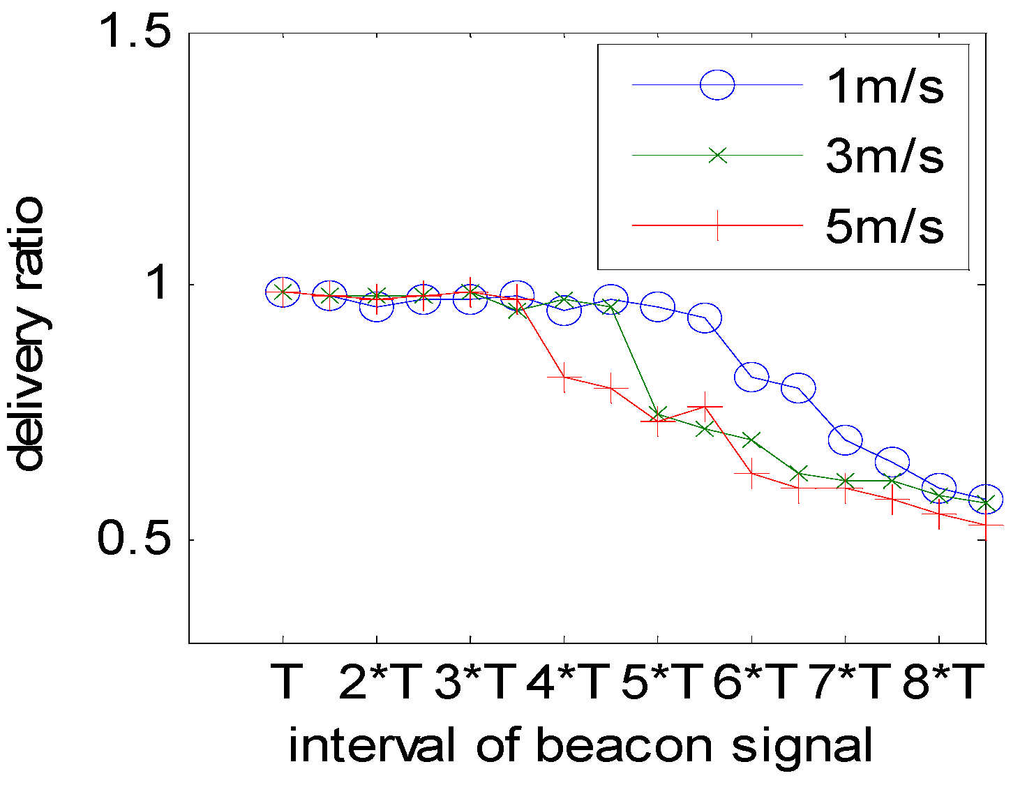
(1) delivery ratio vs. time interval of the beacon signal
The curves of the delivery ratio vs. the time interval of the beacon signal are shown in Figure 11. T represents the propagation time from a sender to a communication radius . We can see the delivery ratio decreases as the interval increases when the speed of water current is 0. When the speed of nodes is 1 m/s and the beacon signal interval is less than 6 T, the delivery ratio is almost same; when the interval is greater than 6 T, the delivery rate decreases significantly. When the speed of nodes is 3 m/s, the delivery ratio starts to decrease at the point of 5 T of the interval of the beacon signal. When the speed of the nodes’ movement is 5 m/s, the point of delivery ratio decrease is 3.5 T. This is because the routing table is unable to be updated in a timely way with the movement of the nodes. In other words, the best next-hop selected may not be the qualified node. In addition, the interval of the beacon signal should be decreased with the increase of the speed of the nodes. So, in the following simulation, the speed of water current is 1–5 m/s and the time interval of the beacon signal is set as 5 T.
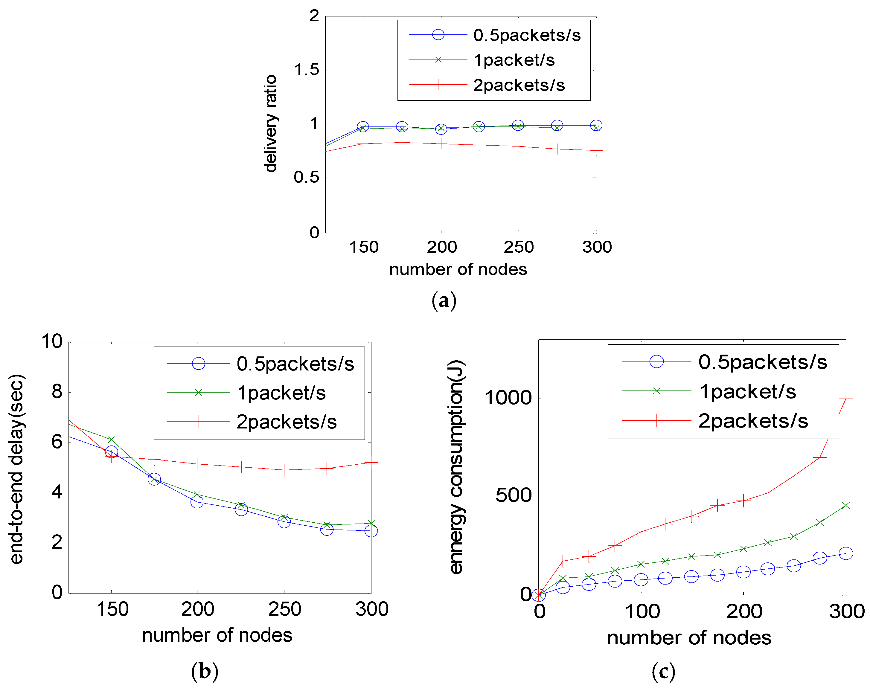
(2) Effect of Data Rate
The packet delivery ratio, energy consumption and end-to-end delay at different data rates are shown in Figure 12. From Figure 12a we can see the delivery ratio increases with the number of nodes when the data rate is 0.5 packets per second and 1 packet per second. The number of candidate next-hop nodes increases as the total number of sensor nodes increases, which results in a better next-hop and a higher delivery ratio. When the data rate is 2 packets per second, the delivery ratio is less than 80%. A high data rate leads to much collision. Figure 12b shows that end-to-end delay decreases as the number of sensor nodes increases, since a more optimized path can be chosen. Figure 12c indicates that the energy consumption is proportional to the number of packets delivered when the data rate is 0.5 and 1 packet per second. When the data rate is 2 packets per second, the energy consumption is more than double that of 1 packet per second, which is due to excessive collisions and retransmission.
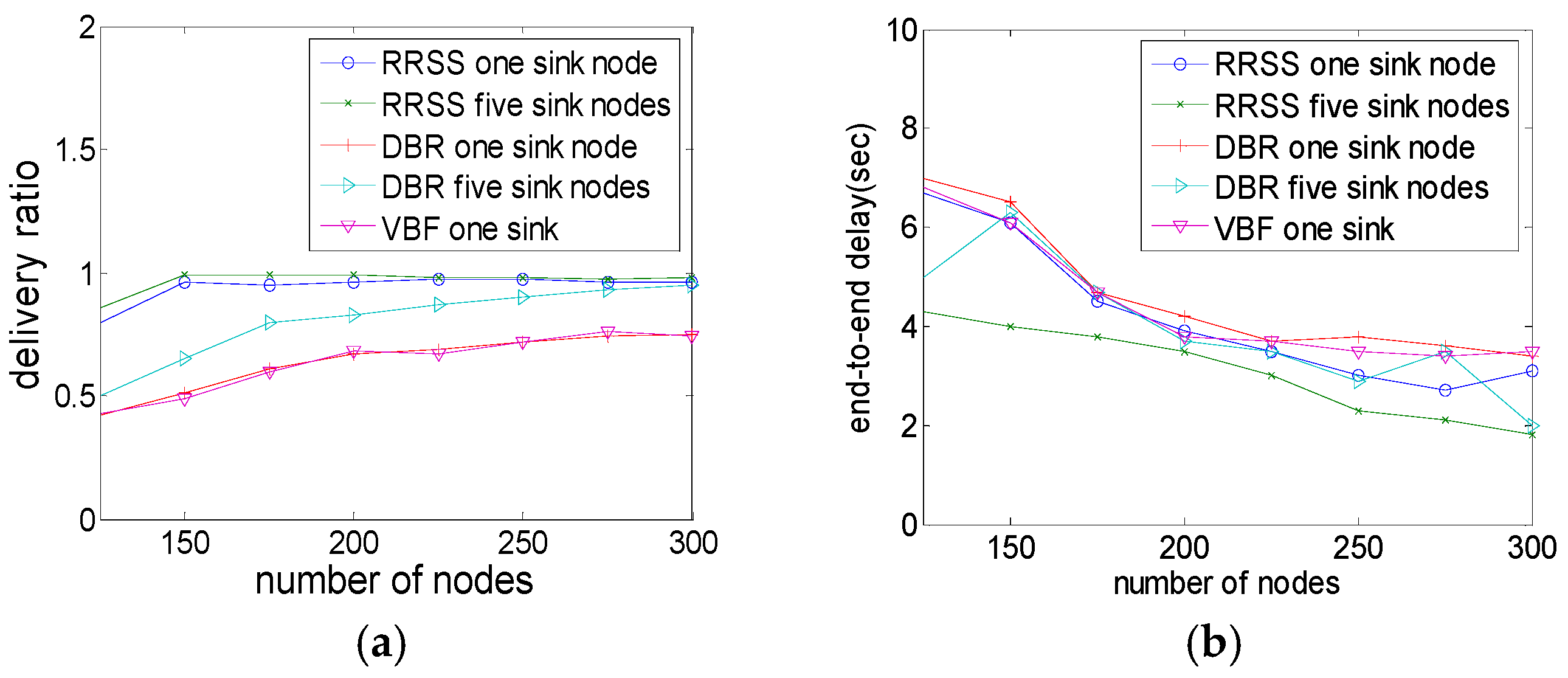
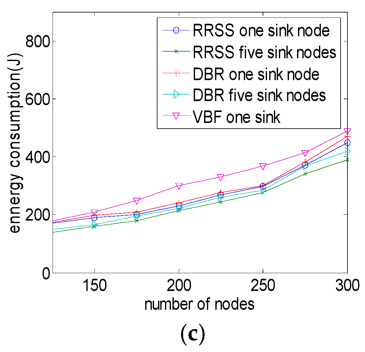
(3) Performance Comparison
In Figure 13, we compare the RRSS with the VBF and DBR routing protocols. Firstly, the delivery ratio is compared in networks with one sink node and five sink nodes, respectively. Figure 13a shows the delivery ratio in the network with five sink nodes is higher than the delivery ratio in the network with one sink node in DBR as well as RRSS. The delivery ratio of RRSS is higher than VBF and DBR, which results from both VBF and DBR being a greedy routing algorithm; and data packets may be forwarded to nodes in void area or without enough residual energy. This can be contrasted with the residual energy and void nodes considered in RRSS. Secondly, we compare energy consumption. Simulation results show that both DBR or VBF consume more energy than RRSS, as in Figure 13b. VBF and DBR are multicast routing. The best next-hop is determined according to the RSSH as well as RSSB in RRSS, and the best next-hop node selected is the nearest to the RSS vector. Thirdly, end-to-end delay with different sink nodes is compared in Figure 13c. Simulation results show that the delay of RRSS is shorter than that of DBR in the network with either five sink nodes or one sink node, which results from the RSS vector reflecting the propagation distance. The shorter the propagation distance, the shorter the end-to-end delay.
6. Conclusions
In UWSNs, a long propagation delay and high energy consumption are important issues. To solve these problems, we propose a novel routing protocol for UWSNs called RRSS. In RRSS, the best next-hop is determined mainly according to receive signal strength. Sink nodes send beacon signal periodically, and a RSS vector is constructed from each underwater node to a sink node according to RSSB. The sender selects the node nearest to the RSS vector as the best next-hop combining the RSSB and RSSH of the neighbor node. To avoid data packets being delivered to the node in void area or with insufficient energy, a void-avoiding algorithm is designed and the energy threshold is preset. Simulation results show the RRSS can decrease delay and save energy consumption compared with DBR and VBF. However, there is still no fundamental solution to the problem of energy balance in UWSNs. In future studies, we need to work hard in this area.
Acknowledgments
This work is supported by the CERNET Innovation Project (NGII20160307), National Natural Science Foundation Projects of China (61162003), Qinghai Office of Science and Technology (2015-ZJ-904), Key lab of IoT of Qinghai (2017-ZJ-Y21), and Hebei Engineering Technology Research Center for IOT Data acquisition and Processing.
Author Contributions
Meiju Li, Xiuxiu Liu and Kejun Huang conceived and designed the experiments; Meiju Li and Senlin Hou performed the experiments; Meiju Li and Xiujuan Du analyzed the data; Xiujuan Du and Kejun Huang contributed analysis tools; Meiju Li wrote the paper.
Conflicts of Interest
The authors declare no conflict of interest.
References
- Heidemann, J.; Ye, W.; Wills, J.; Syed, A.; Li, Y. Research challenges and applications for underwater sensor networking. In Proceedings of the IEEE Wireless Communications & Networking Conference, Las Vegas, NV, USA, 3–6 April 2006; pp. 228–235. [Google Scholar]
- Mohammad, G.S.; Shahrabi, A.; Boutaleb, T. A Novel Cooperative Opportunistic Routing Scheme for Underwater Sensor Networks. Sensors 2016, 16, 297. [Google Scholar]
- Noh, Y.; Lee, U.; Wang, P.; Choi, B.S.C.; Gerla, M. VAPR: Void-Aware Pressure Routing for Underwater Sensor Networks. IEEE Trans. Mob. Comput. 2013, 12, 1676–1684. [Google Scholar] [CrossRef]
- Latif, K.; Saqib, M.N.; Bouk, S.H.; Javaid, N. Energy Hole Minimization Technique for Energy Efficient Routing in Under Water Sensor Networks. In Communications in Computer & Information Science; Springer: Cham, Switzerland, 2013; Volume 414, pp. 134–148. [Google Scholar]
- Ahmed, S.; Khan, I.U.; Rasheed, M.B.; Ilahi, M.; Khan, R.D.; Bouk, S.H.; Javaid, N. Comparative Analysis of Routing Protocols for Under Water Wireless Sensor Networks. arXiv, 2013; arXiv:1306.1148. [Google Scholar]
- Xie, P.; Cui, J.H.; Lao, L. VBF: Vector-Based Forwarding Protocol for Underwater Sensor Networks. In NETWORKING 2006. Networking Technologies, Services, and Protocols; Performance of Computer and Communication Networks; Mobile and Wireless Communications Systems; Springer: Berlin/Heidelberg, Germany, 2006; pp. 1216–1221. [Google Scholar]
- Noh, Y.; Lee, U.; Lee, S.; Wang, P.; Vieira, L.F.; Cui, J.H.; Gerla, M.; Kim, K. HydroCast: Pressure Routing for Underwater Sensor Networks. Vehicular Technology IEEE Trans. Veh. Technol. 2016, 65, 333–347. [Google Scholar] [CrossRef]
- Lee, U.; Wang, P.; Noh, Y.; Vieira, L.F.; Gerla, M.; Cui, J.H. Pressure Routing for Underwater Sensor Networks. In Proceedings of the IEEE INFOCOM, San Diego, CA, USA, 14–19 March 2010; Volume 65, pp. 1–9. [Google Scholar]
- Kiruba, S.J.G. Proficient Transmission of Depth Based Routing and Void-Aware Pressure Routing for Underwater Sensor Networks: Review. Int. J. Adv. Res. Electron. Commun. Instrum. Eng. 2014, 2, 12–18. [Google Scholar]
- Yan, H.; Shi, Z.J.; Cui, J.H. DBR: Depth-Based Routing for Underwater Sensor Networks. In NETWORKING 2008 Ad Hoc and Sensor Networks, Wireless Networks, Next Generation Internet; Springer: Cham, Switzerland, 2008; Volume 4982, pp. 72–86. [Google Scholar]
- Wahid, A.; Lee, S.; Jeong, H.J.; Kim, D. Eedbr: Energy-Efficient Depth-Based Routing Protocol for Underwater Wireless Sensor Networks. In Advanced Computer Science and Information Technology; Springer: Berlin/Heidelberg, Germany, 2011; pp. 223–234. [Google Scholar]
- Coutinho, R.W.; Vieira, L.F.; Loureiro, A.A. DCR: Depth-Controlled Routing protocol for underwater sensor networks. In Proceedings of the Symposium on Computers and Communications, Split, Croatia, 7–10 July 2013. [Google Scholar]
- Ali, T.; Jung, L.T.; Faye, I. End-to-End Delay and Energy Efficient Routing Protocol for Underwater Wireless Sensor Networks. Wirel. Pers. Commun. 2014, 79, 339–361. [Google Scholar] [CrossRef]
- Uddin, M.A. Link Expiration Time-Aware Routing Protocol for UWSNs. J. Sens. 2013, 2013, 625274. [Google Scholar] [CrossRef]
- Basagni, S.; Petrioli, C.; Petroccia, R.; Spaccini, D. CARP: A Channel-aware routing protocol for underwater acoustic wireless networks. Ad Hoc Netw. 2014, 34, 92–104. [Google Scholar] [CrossRef]
- Zhou, Z.; Yao, B.; Xing, R.; Shu, L.; Bu, S. E-CARP: An Energy Efficient Routing Protocol for UWSNs in the Internet of Underwater Things. IEEE Sens. J. 2015, 16, 4072–4082. [Google Scholar] [CrossRef]
- Hwang, D.; Kim, D. DFR: Directional flooding-based routing protocol for underwater sensor networks. In Proceedings of the Oceans, Quebec City, QC, Canada, 15–18 September 2008; pp. 1–7. [Google Scholar]
- Du, X.J.; Huang, K.J.; Lan, S.L.; Feng, Z.X.; Liu, F. LB-AGR: Level-based adaptive geo-routing for underwater sensor networks. J. China Univ. Posts Telecommun. 2014, 21, 54–59. [Google Scholar] [CrossRef]
- Jafri, M.R.; Ahmed, S.; Javaid, N.; Ahmad, Z.; Qureshi, R.J. AMCTD: Adaptive mobility of courier nodes in threshold-optimized DBR protocol for underwater wireless sensor networks. In Proceedings of the 8th IEEE International Conference on Broadband and Wireless Computing, Communication and Applications (BWCCA’13), Compiegne, France, 28–90 October 2013. [Google Scholar]
- Javaid, N.; Jafri, M.R.; Khan, Z.A.; Qasim, U.; Alghamdi, T.A.; Ali, M. Iamctd: Improved Adaptive Mobility of Courier Nodes in Threshold-Optimized DBR Protocol for Underwater Wireless Sensor Networks. In Proceedings of the Eighth International Conference on Broadband and Wireless Computing, Communication and Applications, Tokyo, Japan, 28–30 October 2013; pp. 259–273. [Google Scholar]
- Yang, W.; Kim, D.S. Reliable and energy-efficient routing protocol for underwater acoustic sensor networks. In Proceedings of the International Conference on Information and Communication Technology Convergence, Busan, Korea, 22–24 October 2014; pp. 738–743. [Google Scholar]
- Stojanovic, M. On the relationship between capacity and distance in an underwater acoustic communication channel. ACM SIGMOB Mob. Comput. Commun. Rev. 2006, 11, 41–47. [Google Scholar]
- Thorp, W.H. Analytic Description of the Low-Frequency Attenuation Coefficient. J. Acoust. Soc. Am. 1967, 42, 270. [Google Scholar] [CrossRef]
- Fitzgerald, R.J. The many paths to underwater acoustic communication. Phys. Today 2015, 68, 20. [Google Scholar] [CrossRef]
Figure 1.
Topology 1.

Figure 2.
Network structure.
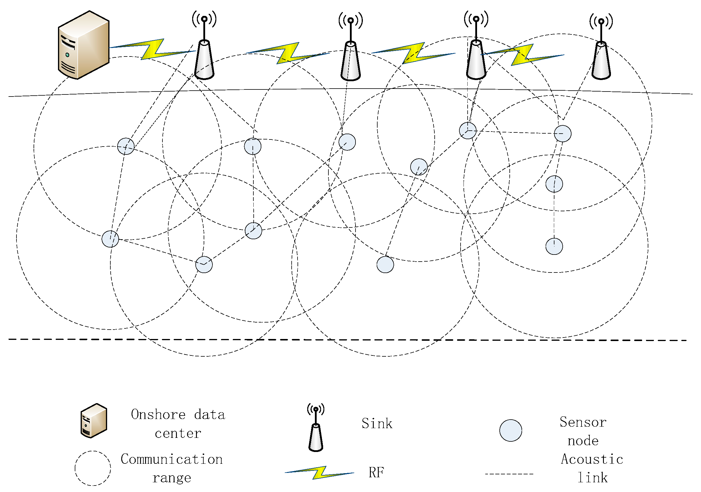
Figure 3.
Topology 2.

Figure 4.
Topology 3.
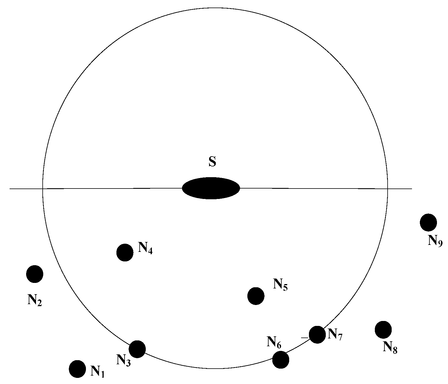
Figure 5.
Topology 4.

Figure 6.
Topology 5.

Figure 7.
Void-avoiding algorithm.

Figure 8.
Candidate area.

Figure 9.
Volume of the candidate area.
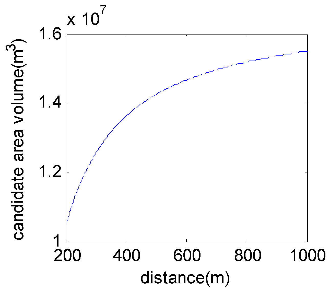
Figure 10.
Topology 6.

Figure 11.
Delivery ratio vs. time interval of the beacon signal.

Figure 12.
Effect of data rate. (a) Delivery ratio vs. the number of nodes; (b) end-to-end delay vs. the number of nodes; (c) energy consumption vs. the number of nodes.
Figure 12.
Effect of data rate. (a) Delivery ratio vs. the number of nodes; (b) end-to-end delay vs. the number of nodes; (c) energy consumption vs. the number of nodes.

Figure 13.
Performance comparison. (a) Delivery ratio vs. the number of nodes; (b) delay vs. the number of nodes; (c) energy consumption vs. the number of nodes.
Figure 13.
Performance comparison. (a) Delivery ratio vs. the number of nodes; (b) delay vs. the number of nodes; (c) energy consumption vs. the number of nodes.


Table 1.
Parameter setting.
| Parameter Name | Value |
|---|---|
| Communication radius | 100 m |
| Data packet payload size | 50 byte |
| Hello packet size | 6 byte |
| Transmission power | 2 w |
| Receive power | 0 w |
| Idle power | 0 w |
| Bit rate | 10 kbps |
© 2017 by the authors. Licensee MDPI, Basel, Switzerland. This article is an open access article distributed under the terms and conditions of the Creative Commons Attribution (CC BY) license (http://creativecommons.org/licenses/by/4.0/).
Share and Cite
MDPI and ACS Style
Li, M.; Du, X.; Huang, K.; Hou, S.; Liu, X. A Routing Protocol Based on Received Signal Strength for Underwater Wireless Sensor Networks (UWSNs). Information 2017, 8, 153. https://doi.org/10.3390/info8040153
AMA Style
Li M, Du X, Huang K, Hou S, Liu X. A Routing Protocol Based on Received Signal Strength for Underwater Wireless Sensor Networks (UWSNs). Information. 2017; 8(4):153. https://doi.org/10.3390/info8040153
Chicago/Turabian StyleLi, Meiju, Xiujuan Du, Kejun Huang, Senlin Hou, and Xiuxiu Liu. 2017. "A Routing Protocol Based on Received Signal Strength for Underwater Wireless Sensor Networks (UWSNs)" Information 8, no. 4: 153. https://doi.org/10.3390/info8040153
Note that from the first issue of 2016, this journal uses article numbers instead of page numbers. See further details here.