A Caching Strategy for Transparent Computing Server Side Based on Data Block Relevance


School of Information Science and Engineering, Central South University, Changsha 410083, China
*
Author to whom correspondence should be addressed.
Information 2018, 9(2), 42; https://doi.org/10.3390/info9020042
Submission received: 13 December 2017
/
Revised: 4 February 2018
/
Accepted: 16 February 2018
/
Published: 22 February 2018
Abstract
:The performance bottleneck of transparent computing (TC) is on the server side. Caching is one of the key factors of the server-side performance. The count of disk input/output (I/O) can be reduced if multiple data blocks that are correlated with the data block currently accessed are prefetched in advance. As a result, the service performance and user experience quality in TC can be improved. In this study, we propose a caching strategy for the TC server side based on data block relevance, which is called the correlation pattern-based caching strategy (CPCS). In this method, we adjust a model that is based on a frequent pattern tree (FP-tree) for mining frequent patterns from data streams (FP-stream) to the characteristics of data access in TC, and we devise a cache structure in accordance with the storage model of TC. Finally, the access process in TC with real access traces in different caching strategies. Simulation results show that the cache hit rate under the CPCS is higher than that using other algorithms under conditions in which the parameters are coordinated properly.
1. Introduction
With the rapid development of pervasive smart devices and ubiquitous network communication technologies, various new network applications and services are emerging continuously, such as Internet of things, virtual/augmented reality, and unmanned vehicles. This trend not only promotes the emergence of mobile content caching, network-aware request redirection and delivery techniques [1,2], but also provides significant opportunities and motivations to the evolution of the computing paradigm. For the server-centric computing paradigms, such as cloud computing, which is characterized by centralized computation and storage, it is difficult to meet the diverse requirements of new network applications and services [3]. Transparent computing (TC) [4] can be viewed as a special kind of cloud computing, yet it is different from the typical cloud computing. TC emphasizes data storage on servers and computation on terminals. Hence, the server stores and manages all the data, which include heterogeneous operating systems (OSs), applications (APPs) and users’ personalized data. Users can obtain OSs and APPs from servers through the network and execute them at their own terminals in a block-streaming manner without considering underlying hardware and implementation details. Therefore, TC offers several advantages: a reduction in user terminal complexity and cost, an improvement in security and user experience, and cross-platform capabilities [5]. In such a service mode, the server side, which is the core of TC, is responsible for the unified storage and management of users’ resources. Meanwhile, it also deals with the resource access request that is sent by users and ensures the quality of service experience. This process may cause numerous input/output (I/O) costs. Thus the major challenge is processing resource requests efficiently and reliably, which may cause numerous I/O costs. A caching mechanism is a widely adopted and effective method to reduce I/O cost [6]. The improvement in cache performance can effectively reduce the I/O overhead in the TC server, thereby improving the efficiency for users accessing server resources, and enhance the user experience. There have been some works on improving the performance of the TC server. A caching strategy called frequency-based multi-priority queues (FMPQ) was proposed in [7]. FMPQ can adapt to different cache sizes and workloads under the TC environment. Tang et al. [8] propose a block-level cachingoptimization method for the server and client by analyzing the system bottleneck in mobile TC. In consideration of the limited size of the server memory and the dependency among files, the authors of [9] proposed a middleware to optimize the file fetch process in the TC platform. To evaluate the performance of TC services and the cache hit rate of the multi-level caching structure, a simulation framework (TranSim) was implemented in [10]. In summary, the existing research on the cache of the TC server almost only considers the traditional factors, such as timeliness, access frequency and cache structure. There is no research that focuses on the relevance of data blocks in TC.
In the process of developing a caching strategy, the prefetching strategy is a key influence factor. If the data blocks can be prefetched accurately, the number of disk I/Os will be reduced effectively, and the cache hit rate will be improved. Therefore, if the association rules between data blocks are determined by mining frequent item sets from the historical data, the accuracy and efficiency of prefetching can be effectively improved. Lin et al. [11] proposed a fastand distributed algorithm for mining frequent patterns in congested networks (FDMCN) based on the frequent item mining technology. The traditional frequent pattern mining algorithms are only suitable for static data. For example, the Apriori algorithm [12] explores frequent item sets by traversing, connecting with, and pruning the original data repeatedly. The costly generation of candidate sets makes it impossible to mine out frequent item sets in time. Mining frequent patterns by pattern fragment growth (FP-growth) [13] improves the method of processing data by scanning the original data twice, so that the efficiency is increased. However, it is also limited by time and space when it is applied to a large amount of fast and uncertain stream data. The users’ data access request for TC servers is transmitted in the form of a data stream. Therefore, such static frequent pattern mining algorithms are not suitable for TC APPs. Algorithms that explore frequent item sets in data streams can mine and update frequent patterns dynamically, with limited computation and storage capacity. Thus frequent pattern mining in data streams has become a popular topic in data mining research [14,15]. Much research has analyzed the problems in the processing of time data streams based on FP-trees. Chen et al. [16] designed a mining algorithm based on a weighted FP-tree. Itintroduces the weight characteristics into the FP-growth mining algorithm, making it more suitable for the calculation process of the time FP-stream. Ölmezoğulları et al. [17] added Apriori and FP-growth algorithms for stream mining inside an event processing engine. The FP-stream [18] is one of the algorithms that dynamically updates frequent item sets with the incoming data streams. In the FP-stream algorithm, frequent patterns are compressed and stored by using a tree structure that is similar to the FP-tree. To mine and update frequent patterns in a dynamic, data stream environment, the FP-stream actively maintains frequent patterns under a titled-time window framework to summarize the frequent patterns at multiple time granularities.
In this paper, we first introduce the properties of TC and the pertinence among the data blocks in TC in Section 2. According to the data access characteristics of the transparent server side, we adjust the FP-stream and propose a caching strategy called the correlation pattern-based caching strategy (CPCS) in Section 3. The kernel idea of the CPCS is to prefetch as many data blocks as possible from the virtual disk (Vdisk) into the cache by mining the correlation among data blocks in TC in real time. Section 4 presents the experiment, in which the effectiveness of the CPCS was evaluated by simulating the process of accessing a TC server. Section 5 concludes this paper.
2. Preliminary
The TC system consists of a transparent server, transparent terminals and the transparent network. Transparent terminals are devices that only contain essential hardware for computing and I/O. Instead of OSs and APPs, there are just fundamental basic I/O system (BIOS), a few protocols and supervisory programs. Users request services without considering heterogeneity among software, thereby autonomously choosing the software service they really need. The transparent server is always a computing device or supercomputing centre that carries external storage. The server not only takes charge of the coordination among transparent terminals and the monitoring of the TC system, but also stores various software that users need, and receives and distributes all information resources. Huge amounts of data that are accumulated from terminals and relay platforms are processed rapidly on the server. Thus, information in terminals, relay platforms and command platforms can be transferred seamlessly in real time [4,5,19]. Compared with cloud computing, TC efficiently improves the maintainability and security of the whole system by taking full advantage of the computing resources on the client side and emphasizing the cloudification of the software on the server side [20].
The transparent computing platform (TCP), which is implemented on the basis of Vdisks, is the core of the transparent server. The TCP takes charge of the management and allocation of OS resources, application resources and users’ private resources, by providing data storage and access services for the terminal users through the transparent network. All the requests that come from terminals are redirected to the Vdisks in the TCP [21].
All the resources are organized and stored on the TCP in the form of Vdisk data. The storage model of the Vdisk in the TCP presents a tree-like structure by dividing data into three groups on the basis of data-shared degrees. The top-most node of the tree is the Vdisk image about systems (S_VDI), where resources can be shared by all users. Data in S_VDI are used for loading systems. The next layer down is the Vdisk image about APPs (G_VDI), where resources are shared by users having something in common. At the bottom of the tree is the Vdisk image about terminal users (U_VDI), where resources belong to individuals. Data in U_VDI are users’ private files and personalized modifications to shared resources.
Redirect-on-write [22] is used for enforcing data consistency in the TCP. When multiple terminals have accessed the same system or application at the same time, data in S_VDI and G_VDI are available to all users in read-only mode. If one user needs to modify the data in S_VDI and G_VDI, the rewritten data block will be stored in the user’s U_VDI with redirect-on-write. The system judges whether one shared data block has been rewritten or not quickly, through marking the rewritten data block with bitmap [23] rather than by searching the entire table. Bitmap marks data blocks that have never been modified with 0, and marks data blocks that have been modified with 1.
Attributed to the storage model of TC that divides data into three groups, the data in S_VDI and G_VDI can be accessed centrally and closely, particularly when there are many users operating intensively in TC. The data blocks that may be interrelated to each other can be accessed continuously in a short time. Therefore, a prediction for the block relevance is favorable to the prefetching in a caching strategy. Moreover, a cache structure that corresponds to the storage model of TC is beneficial for promoting the efficiency of data matching in the cache.
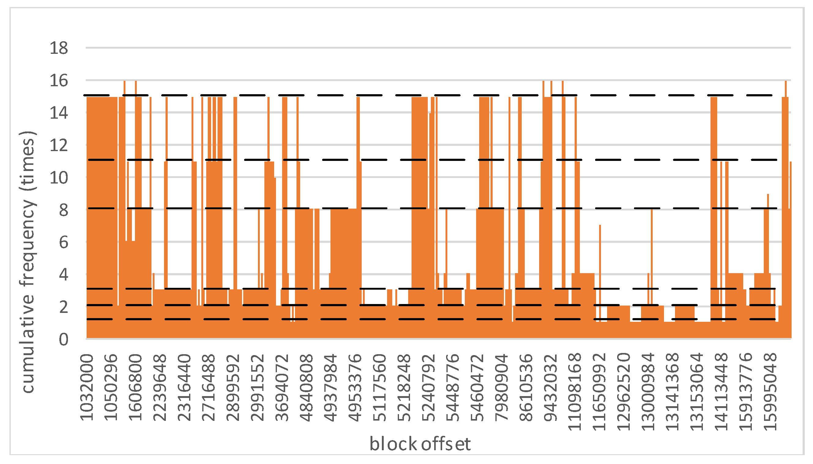
The TCP keeps the data access traces in TC, in which one record denotes that a data block is accessed once. Every record contains the access time and the offset of one block. We randomly draw 5 min access records in TC. For each data block that appears in these records, we count up the cumulative access frequencies and plot a histogram, as shown in Figure 1. For example, a rectangle with coordinate (1,032,048, 14) indicates that the data block whose offset is 1,032,048 has been accessed 14 times during the 5 min. Figure 1 shows that almost all the cumulative frequencies are among 1, 2, 3, 8, 11 and 15. The frequencies 1, 2 and 3 indicate that a large number of data blocks are accessed occasionally. For the data blocks that have been accessed with a high frequency, such as 15, 11 or 8, they are accessed synchronously with a high probability. Hence, it is supposed that there are strong association rules among these data blocks. With the characteristics of TC, this paper solves the problem of how to discover strongly related data in real time by mining frequent patterns and provides evidence for drawing up more effective caching strategies.
3. Caching Strategy Based on Relevance
In this section, the details and properties of the FP-stream are analyzed. To make it suitable for the caching strategy on the TC servers, we make some adjustments to the FP-stream. Then a caching strategy that is based on frequency patterns is proposed. In this method, the cache structure is related to the storage model of TC. We call the changed FP-stream the TCFP-stream. Thus the FP-tree structure in the TCFP-stream is called the TCFP-tree, and the patten-tree structure is called the TC-pattern-tree.
3.1. Description of FP-Stream
We suppose the transaction database contains a set of transactions for some time. is a transaction that includes different items, where . All the items in come from the item set . If A is one of the subsets of I, then the present frequency of A in DB is called the support count of A. The support of A is a calculation of the support count of A to the size of DB.
Definition 1.
The item set A is a frequent pattern as long as the support of A is no less than the minimum support, which is a predefined threshold.
The FP-stream [18] is based on the FP-tree [13], applying the method of mining frequent patterns to data streams. The FP-stream splits the data stream into a number of batches in chronological order. Batches are processed as static transaction databases over different time periods with FP-growth. By processing data in batches, the FP-stream relieves conflicts between the limitation of computing space and the hugeness of the data volume. There are two main data structures: the FP-tree and the pattern-tree. The FP-tree is used for compressing original data in each batch and mining frequent patterns periodically. Every time it comes to the end of one batch, the FP-tree will be emptied to make space for the data in the coming batch. All the frequent patterns and timing relationships are retained by scanning the original data twice. A pattern-tree is used to retain all the frequent patterns that are mined from each batch of data. The data structure of the pattern-tree is shown in Figure 2. Generally, people are more interested in recent events than remote events. In the pattern-tree, time information about frequent patterns is stored in titled-time windows, where the latest data are stored at the most granular level and the older data are stored at a much more coarsely grained level. The support count in the time-sensitive window indicates the support count of the frequent pattern, which consists of all the nodes from the root to the current node. With the titled-time window frame, the FP-stream does not only retain all the effective frequent patterns, but it also fits into the interest tendency of people [24].
In the data stream, some item sets may become frequent patterns in later batches, even if they are not currently. The FP-stream introduces the maximum support error to largely avoid missing frequent patterns, which promises that the frequent patterns are always unabridged. We suppose the minimum support, the maximum support error and the width of the batch are , and , respectively. The steps as follow show the process in which the FP-stream mines and retains frequent patterns.
- Build FP-tree and mine frequent patterns.
- (a)
- Scan the current batch of data , and create the header table f_list according to the frequency of items in . If , only the items whose support counts are larger than are stored in f_list. If , all the items in are stored in f_list with their support counts, without filtering.
- (b)
- The FP-tree is a prefix tree storing compressed data information from each batch of data. If the FP-tree is not null, empty the FP-tree. Sort each transaction in according to the item order in f_list, and compress sorted data into the FP-tree from the root.
- (c)
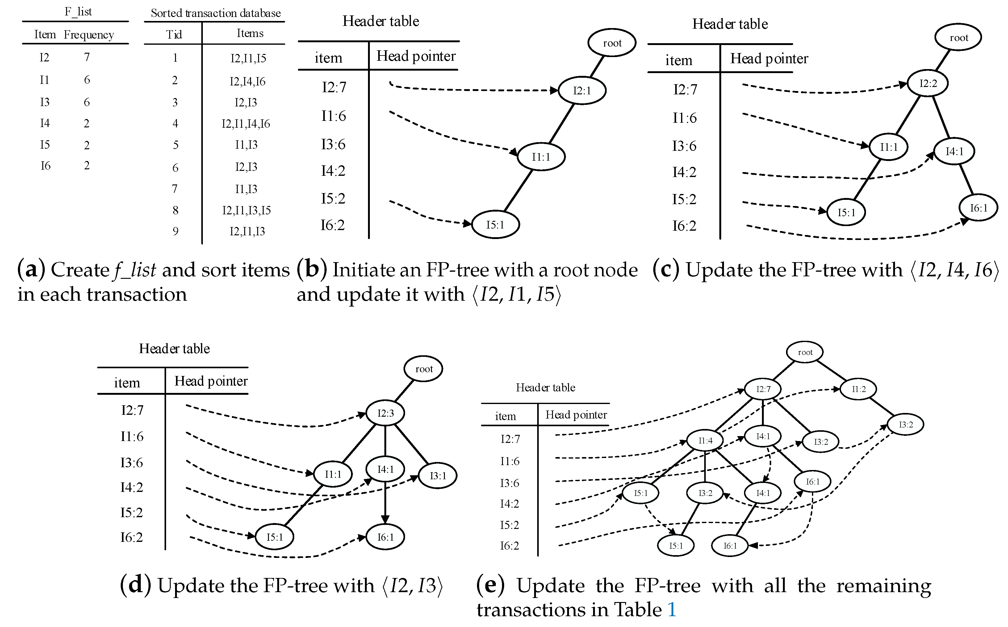
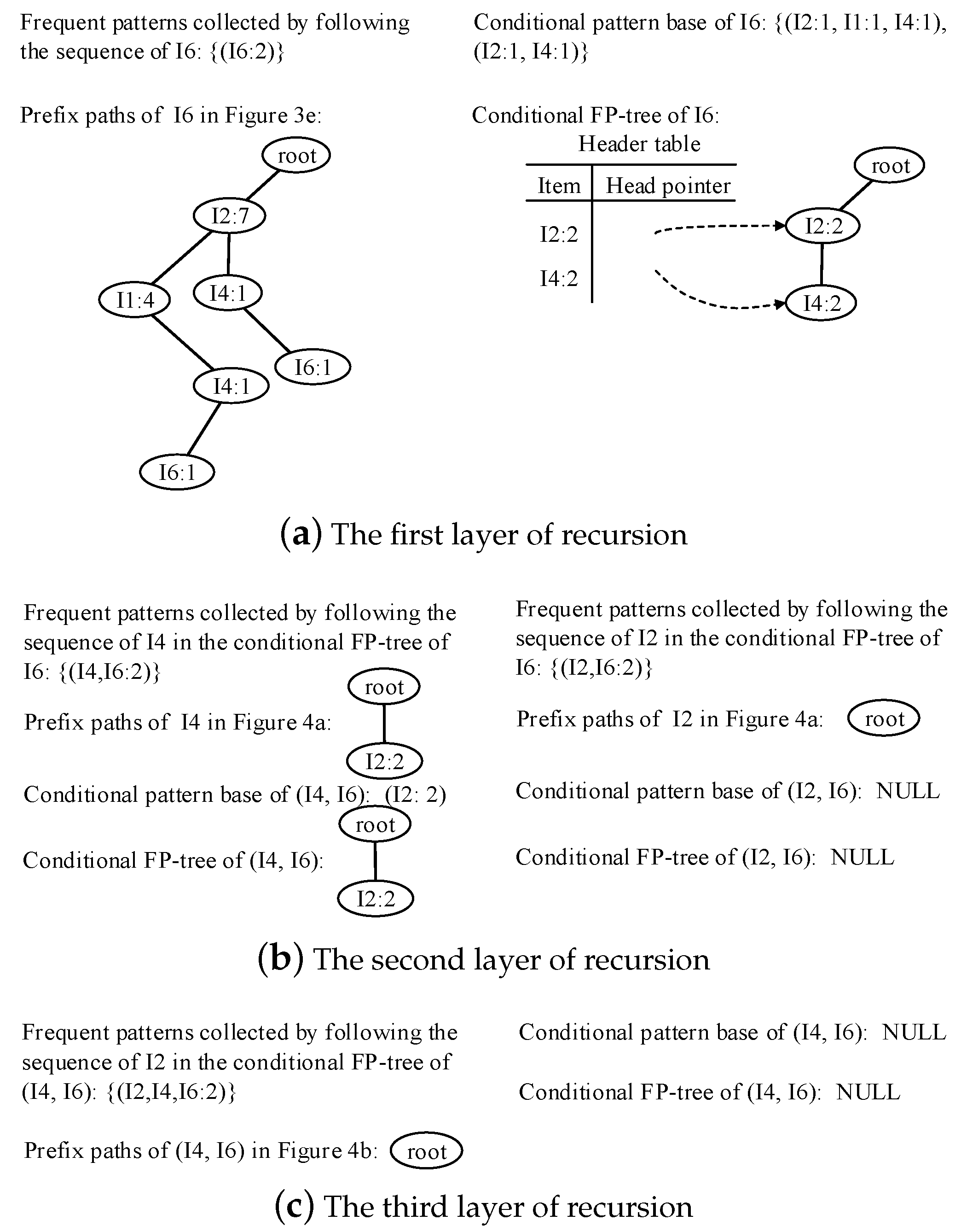
- Traverse the FP-tree from the node corresponding to the last item in f_list with FP-growth. Mine frequent patterns out gradually while the FP-tree is essentially producing one level of recursion at a time, until recursion to the root.Example 1.Suppose the minimum support is 0.2 and the maximum support error is 0.01. If the data in Table 1 are one batch of original data, where data are recorded as some transactions, we can build an FP-tree with these data following the steps shown in Figure 3. Here, frequent items are the items whose support count is not less than in the transaction database. First, the transaction database is scanned once, and the f_list is created with frequent items in descending-frequency order. Then items in each transaction are sorted according to the sequence in f_list. The created f_list and sorted transaction database are shown in Figure 3a. Next, the sorted transaction database is scanned individually, and the FP_tree is initiated. An empty node is set as the root node of the FP_tree. Figure 3b shows that the first transaction is used to build a branch of the tree, with the presented frequency 1 on every node. The second transaction has the same prefix as the first transaction. Thus the frequency of the node (I2:1) is incremented by 1. The remaining string derives two new nodes as a downward branch of 〈I2:2〉, with presented frequency 1. The results are shown in Figure 3c. The third transaction has the same prefix as the existing branches. Thus the frequency of the node (I2:2) is incremented by 1 again, and derives a new node as the child node of (I2:3), with frequency 1. By analogy, an FP-tree can be built as shown in Figure 3d with all the data in Table 1. Every time a new node is created, it will be linked with the last node that has the same name as the new node. If there is no node to link, the new node will be linked with the corresponding head pointer in the header table. Following these node sequences starting from the header table, we can mine out complete frequent patterns, for example, from the FP-tree in Figure 3e. This starts from the bottom of the header table.The process of mining frequent patterns based on I6 are shown in Figure 4. Figure 3e shows that I6 is at the bottom of the header table. Following the sequence that starts from I6 in the header table, we can obtain two nodes with the name I6, and both of them have the frequency count 1. Hence, a one-frequent-item set can be mined out: . In Figure 3e, there are two prefix paths of I6: and . As the number of times I6 appears, the paths indicate that items in the strings and have appeared once together. Hence, just the paths and count when the mining is based on I6. Then is called I6’s conditional pattern base. With the conditional pattern base of I6, the conditional FP-tree of I6 can be built as shown in Figure 4a. Because the accumulated frequency of I1 in is 1, which is less than the minimum support count of 1.71, I1 is discarded when the conditional FP-tree of I6 is built. So far the first layer of recursion has finished. The second layer of recursion starts from scanning the header table in the conditional FP-tree of I6. Figure 4b shows the second layer of recursion. Similarly to the analysis of I6 in the global FP-tree that can be found in Figure 3e, the second layer of recursion is based on I2 and I4 in the conditional FP-tree of I6. Thus the second recursion involves mining two items I4 and I2 in sequence. The first item I4 derives a frequent pattern (I4, I6:2) by combining with I6. Next, the conditional pattern base and conditional FP-tree of (I4, I6) can be created according to the prefix path of I4 in the conditional FP-tree of I6. With the conditional FP-tree of (I4, I6), the third layer of recursion can be derived. The second item I2 derives a frequent pattern (I2, I6:2) by combining with I6. Then the conditional pattern base and conditional FP-tree of (I2, I6) can be created according to the prefix path of (I2) in the conditional FP-tree of I6. In fact, the parent node of (I2) is a root node; thus the search for frequent patterns associated with (I2, I6) terminates. Figure 4c indicates that the third layer of recursion is based on I2 in the conditional FP-tree of (I4, I6). The item I2 derives a frequent pattern (I2, I4, I6:2) by combining with (I4, I6). Because the parent of (I2) is the root node, the search for frequent patterns associated with string (I2, I4, I6) terminates. By traversing the FP-tree in Figure 3 with FP-growth, the frequent patterns mined out are presented in Table 2.
- Update time-sensitive pattern-tree on the basis of the frequent patterns that have been mined out in step 1.
- (a)
- Every time we come to the end of the data batch, update the pattern-tree with the frequent patterns that have been mined out in step 1. Suppose one of the frequent patterns is I. If I has existed in the pattern-tree, just update the titled-time window corresponding to the frequent pattern I with its support count. If there is no path corresponding to I in the pattern-tree and the support count of I is more than , insert I into the pattern-tree. Otherwise, stop mining the supersets of I.
- (b)
- Traverse the pattern-tree in depth-first order and check whether or not each time-sensitive window of the item set has been updated. If not, insert zero into the time-sensitive window that has not been updated.
- (c)
- Drop tails of time-sensitive windows to save space. Given the window that records the information about the latest time window, the window that records the information about the oldest time window, and the support counts , , , …, , which indicate the present frequencies of one certain item set from to , retain , , , …, and abandon , , , …, as long as the following condition is satisfied:
- (d)
- Traverse pattern-tree and check whether or not there are empty time-sensitive windows. Drop the node and its child nodes, if the node’s time-sensitive window is empty.
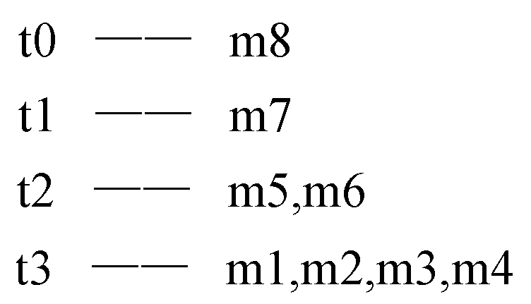
In the titled-time window, if one slot keeps transactions in the current minute, the next three slots keep transactions in the last minute, two minutes earlier and four minutes before the two. Thus time granularity increases exponentially with base 2, and one year of data only needs units of time windows to store. If the algorithm has processed the data stream for 8 min and every minute can be represented as m1, m2, m3, m4, m5, m6, m7 and m8 from the beginning, the time periods in Figure 2 can be mapped as shown in Figure 5.
On the basis of the above steps and analysis, we can draw the conclusion that the FP-stream can store many frequent patterns with little space. However, problems also exist. When the effective frequent patterns emerge gradually as the recursion goes on, a number of subsets come concomitantly, which take up more time and space because of the titled-time window frame. Additional subsets are useless and redundant for the original intention to improve the cache performance by prefetching maximal frequent patterns of blocks. For example, in Table 2, the item sets , and are the subsets of and have the same frequency count as . There are three redundant item sets along with one effective item set. On account of this phenomenon and the characteristics of the TC server accessing data, Section 3.2 provides improvements to the FP-stream algorithm.
3.2. Optimizing the FP-Stream
The idea of this paper is to improve the cache performance of the TC server by prefetching as many data blocks correlated strongly to the data blocks requested currently as possible. In this section, we have made some changes to the FP-stream to mine frequent patterns effectively and efficiently. These changes can be viewed from two aspects: mining frequent patterns and processing batches.
The first aspect is mining frequent patterns. The performance of caching depends on replacing useless data with useful data. Useful data depend on effective frequent patterns. Effective frequent patterns are those frequent patterns without supersets having the same frequency count. However, according to the above analysis of the FP-stream, if the set of data blocks prefetched is capacious, there will be plenty of subsets when frequent patterns are explored with FP-growth. We suppose there is one single path P consisting of n nodes, and all the nodes in this path have the same frequency count; n is large enough. When we mine out frequent patterns from P with FP-growth, the number of frequent patterns to be mined out, conditional FP-trees to be created, and items to be processed during the top three recursions are shown in Figure 6.
In the first recursion, the mining starts from the bottom of the header table of P. Then it involves n items in sequence from the bottom to the top. Combined with the suffix items, the n items derive n frequent patterns. Next, each of the n items derives a conditional pattern base and a conditional FP-tree. All the conditional FP-trees only have one single path. According to the length of every conditional pattern base derived, the numbers of items needed to build the conditional FP-trees are , respectively. Thus there are at least operations to build n conditional FP-trees in the first recursion. The second recursion is to mine frequent patterns from the n conditional FP-trees built in the first recursion. Because there are nodes in the conditional FP-trees, respectively, items in the header table of these conditional FP-trees derive frequent patterns. Then the conditional pattern bases of the items in these conditional FP-trees built in the first recursion will derive conditional FP-trees for the second recursion, during which there are operations. By analogy, the third recursion will derive frequent patterns, conditional FP-trees and needs at least operations. Similarly, recursion is continued to the nth layer, where the conditional FP-tree is null.
From the above analysis and calculation, with the layer of recursion increasing, the time complexity increases. The increasing length of one single path also makes the number of frequent patterns increase. Hence, to make the FP-stream better suited for the caching strategy in TC, we need to abnegate some subsets when mining frequent patterns, particularly the one-item frequent patterns. The details are as follows.
During the process of mining the FP-tree recursively with FP-growth, once there is a single prefix path and all the nodes in this path have the same frequency count, the mining of the prefix path of the current conditional FP-tree stops. All the items appearing in the path can be combined together as an effective frequent pattern. Moreover, to avoid outputting a one-item frequent pattern, during the process of dealing with each item in the header table of the global FP-tree, the step exporting one-item frequent patterns is skipped. Algorithm 1 describes the details of how to mine frequent patterns from the FP-tree with the changed FP-growth. Because of the change to the method of mining frequent patterns from a single path, one step is needed to complete the data-mining task, if we fetch items in this single path as the last frequent patterns directly. Thus no matter how many nodes the single path has, the time complexity is always , and the space taken up is just for one item set.
| Algorithm 1: Mining frequent patterns with changed FP-growth. |
| Input : An FP-tree constructed by original data: FP-tree. Output: Frequent patterns. 1 Tree ← FP-tree; ← null; 2 if Tree contains a single path p and all nodes in the path p have the same support s then 3 denote the combination of the nodes in the path p as ; 4 generate pattern with support s; 5 return; 6 else 7 for each in the header of Tree do 8 generate pattern with support ; 9 if α is not null then 10 output frequent pattern ; 11 end 12 construct conditional FP-tree ; 13 if is not null then 14 Tree ; 15 mine frequent patterns out of from the second row in Algorithm 1; 16 end 17 end 18 end |
We call the changed FP-stream the TCFP-stream. Then the FP-tree structure in the TCFP-stream is called the TCFP-tree, and the patten-tree structure is called the TC pattern-tree. On the basis of the assumptions in Example 1, namely, that the minimum support is 0.2, the maximum support error is 0.01 and the data in Table 1 belong to the first batch; frequent patterns can be mined out with Algorithm 1, as shown in Figure 7. The process of building a TCFP-tree is unaltered, and thus Figure 7 still takes the frequent patterns of I6 in Figure 4e as an example. It starts from the bottom of the header table. Although the one-item frequent patterns (I6:2) are collected first, they are not exported. With the prefix paths of (I6), the conditional pattern base of I6 is determined. Then the conditional TCFP-tree of (I6), in which there is a single path, is shown in Figure 7. Items that are related to the nodes in the single path constitute a frequent pattern: (I4, I2, I6:2). The process of mining frequent patterns about I6 terminates. Similarly, the frequent patterns that are related to other items in the header table are mined out, and they are shown in Table 3.
However, subsets’s being left out also has a knock-on effect. If we mine the frequent patterns with FP-growth, all nodes in a pattern-tree will have titled-time windows, except for the root node. While we mine frequent patterns with Algorithm 1, the titled-time windows of nodes that belong to subsets that have been left out will not be updated in time. Then there will be problems in the later steps, during which the node is dropped as long as its titled-time window is empty. To solve this problem, when we update the pattern-tree, as for the frequent pattern whose subsets have been left out, we update titled-time windows of all nodes in the prefix path with the same value, which is in fact the support count of the maximum frequent patterns. However, this method may weaken the relevancy among items in the subset if the support count of the subset is greater than that of the maximum frequent pattern. This it is necessary to update the time window of the subset. To identify which batch of data the current item set comes from, a new field that is named bat is added to the titled-time window frame. Thus the number of the current batch can be recorded in bat. When a coming frequent pattern is one subset and its superset has been recorded in the pattern-tree, the record in the titled-time window is to be replaced with the true support count, as long as the value of bat is equal to the number of the current batch and the support count of the subset is greater than that of its superset. Example 2 shows the details of building a pattern-tree. Additionally, the influences on the process, which come from the changes in mining frequent patterns, are also introduced with specific data.
Example 2.
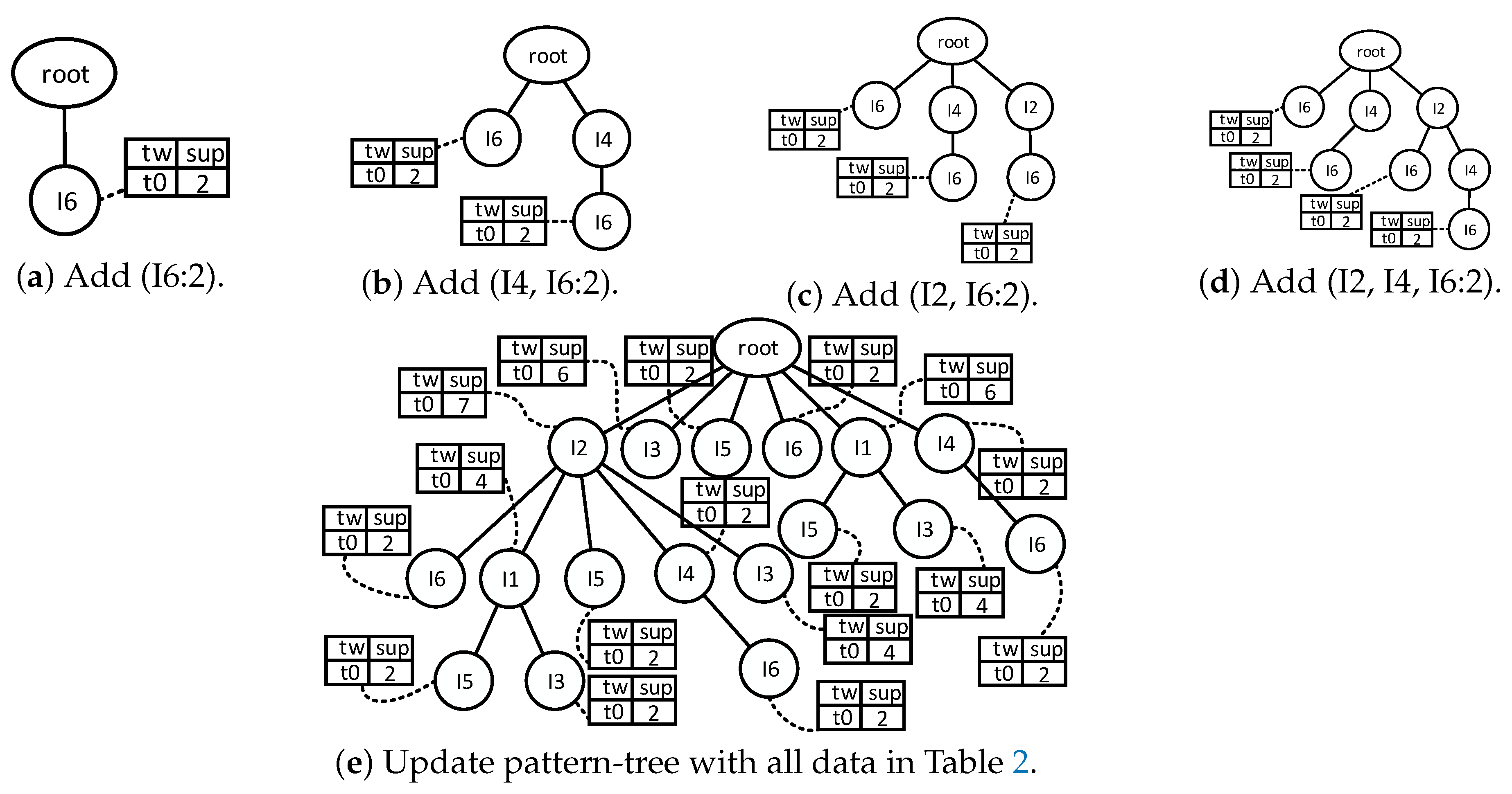
As for the FP-stream algorithm in [18], a pattern-tree can be built with the frequent patterns in Table 2. The process is shown in Figure 8. Because the data in Table 1 are the first batch of data, the initial pattern-tree only has a root node. Before updating the pattern-tree, items in each frequent pattern are sorted according to the order in the header table. Then the pattern-tree is updated by the frequent patterns in turn. The first frequent pattern is (I6:2). Figure 8a indicates that a new node whose name is I6 is created as one child node of the root node. The related titled-time window records the support count 2. The second frequent pattern is (I4, I6:2). Although it has the same item I6 and support count 2 as the first frequent pattern, it is necessary to create a new branch from the root, because the first item in (I4, I6:2) is not I6 according to the order in the header table. Figure 8b shows the pattern-tree that has been updated by (I4, I6:2). The next frequent pattern is (I2, I6:2), and the result is shown in Figure 8c. As for (I2, I4, I6:2), it shares the prefix (I2) with (I2, I6:2); thus two new nodes follow the node (I2), as Figure 8d shows, and so on. Figure 8e shows the pattern-tree that has been updated by all data in Table 2. Up to this point, all frequent patterns that come from the first batch of data have been retained in a pattern-tree. Frequent patterns that come from the batches after the first batch will also be added to this pattern-tree, and their support counts will be recorded in the next elements of the time-sensitive window. From Figure 8, we can see that all the nodes have a time-sensitive window, except the root node.
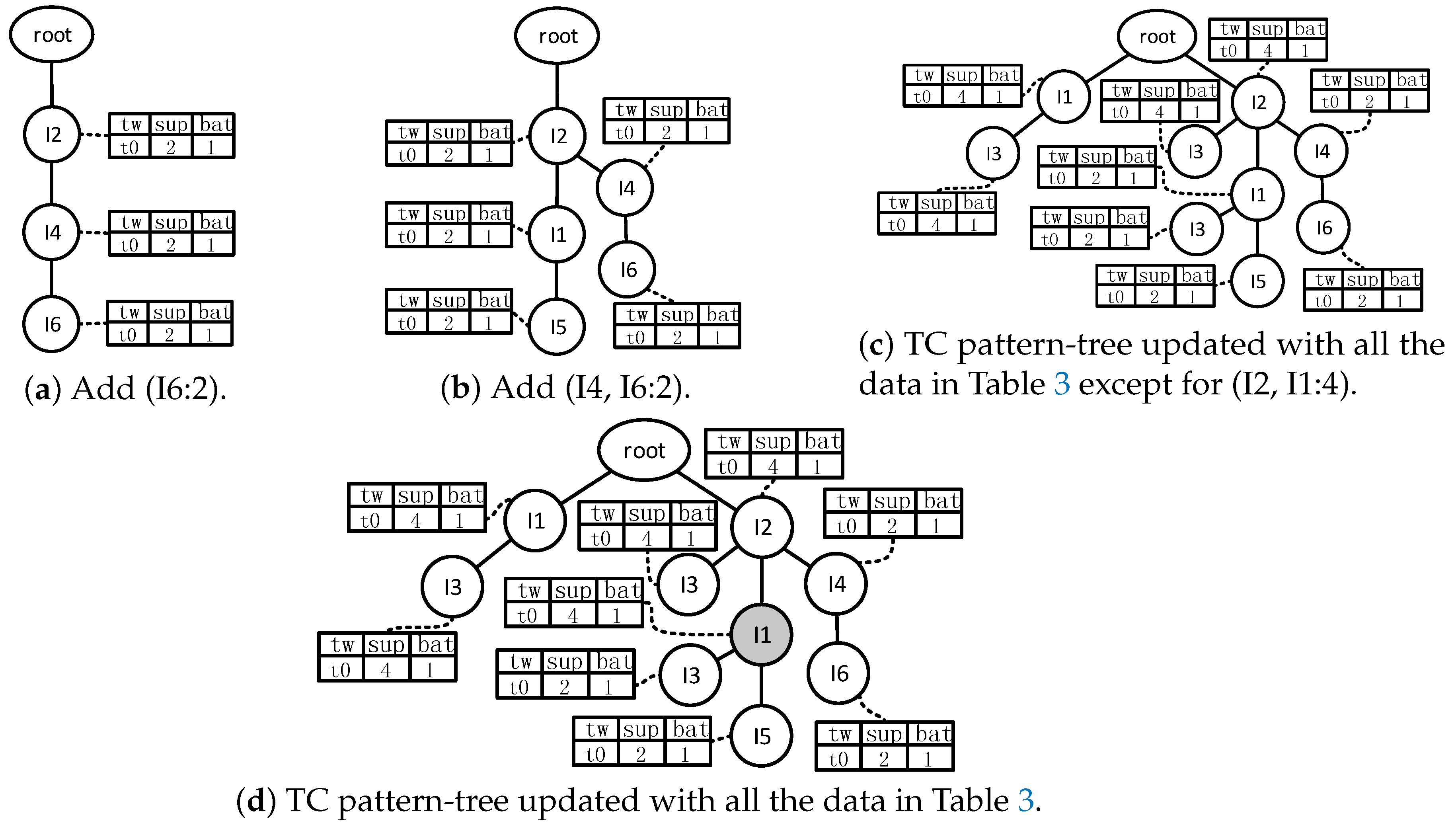
Because Table 2 contains all the frequent patterns and the subsets, all nodes in Figure 8e have titled-time windows. Nevertheless, there will be many nodes without a titled-time window if the pattern-tree is built with the data in Table 3. Figure 9 shows the process of building a TC pattern-tree. The first frequent pattern is (I2, I4, I6:2). Three nodes are created and added into the initial TC pattern-tree, which consists of one root node. The support counts of all the nodes that exist in this path are updated by 2, besides (I6). Figure 9a shows the TC pattern-tree that has been updated by (I2, I4, I6:2). Similarly, Figure 9b shows the TC pattern-tree that has been updated by the second frequent patten (I2, I1, I5:2). The next is (I2, I4:2). The TC pattern-tree is unaltered on account of that (I2, I4:2) and (I2, I4, I6:2) share the same prefix (I2, I4) and the same support count. As for the next three frequent patterns, the result of updating the TC pattern-tree is shown in Figure 8c. The last frequent pattern (I2, I1:4) is a subset of (I2, I1, I3:2). The support count of (I2, I1) was updated when the TC pattern-tree was updated by (I2, I1, I3:2). However, the support count of (I2, I1, I3:2) is smaller than that of (I2, I1:4), and both of the two frequent patterns come from the same batch of data; thus the support count of (I2, I1:4) is incremented to 4, as shown in Figure 9d. Then the effective item sets are retained.
The second aspect is about processing batches. In the FP-stream, the original data are compressed in an FP-tree without filtering, if the current batch is not the first batch. The coming data take up a good amount of time and space to store, although FP-tree is a highly condensed and smaller data structure. Hence, changes on the batch are made, on the basis of the characteristics of TC.
Random 5 min true access records have been fetched to analyze the timeliness of accessing data on the TC server side. Every record included the access time and the accessed data block. Only records that involved blocks that had been accessed over 15 times during the 5 min were retained. There were 2878 different data blocks involved in the 43,225 records left. We grouped these records on the basis of the rule that records sharing the same data block were grouped together. Then the records were sorted by time in each group. Next the intervals between the contiguous records were calculated in each group, which indicated the interval for how long one block would be accessed again since it was accessed the last time. We obtained a distribution of accessing intervals as shown in Figure 10 by putting all the intervals together and counting on the basis of the extent. For example, the first column indicates that 14,135 accessing intervals were no more than 5 s. Thus a block could be re-accessed 5 s after the last access, and the probability was calculated as 14,135 with the classical probabilistic model.
Figure 10 shows that the intervals were highly dispersed, with values ranging from 0 to 35 s. Therefore, the time interval for how long heavily requested data blocks were accessed again since this time was not long. Thus the data access in the TC server is local for time. This phenomenon inspires us to make some changes to the FP-stream. In the FP-stream, if the current batch of data is not the first batch, the algorithm will retain all the items, whether the items are accessed frequently or not. Under the circumstances, a large number of data blocks, which are not accessed frequently, will be dropped from the pattern-tree shortly after being put in the pattern-tree. The repeating processes result in waste in terms of time and space.
On account of the above analysis, we introduce a parameter for the FP-stream, referring to the fact that the access interval of heavily requested data is not long and to the objective that effective frequent patterns are retained while resource consumption is reduced. If the current batch of data is not the first batch, instead of retaining all the items present in the transaction database, we only save the items that have been present more than times by compressing data into the FP-tree. Here is an elasticity coefficient that controls the amount of data to be retained. The smaller is, the larger the amount of data to be processed. Thus the FP-stream algorithm will take up more time and space. On the contrary, the larger is, the less time and space the algorithm will take up. However, although time and space resources can be saved when is very large, some frequent patterns will be missed in the case that is not large enough. Therefore, the value of is supposed to be adjustable in light of the accessing distribution and cache configuration.
3.3. Caching Strategy
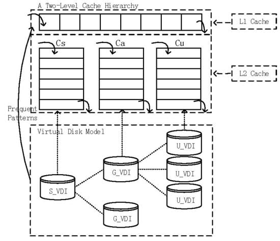
We propose a two-level cache structure and the CPCS, on the basis of the TCFP-stream and the storage model of the TC server.
The cache structure is shown in Figure 11. In the two-level cache structure, the first level of the cache, L1, consists of one queue, which stores the frequent patterns that are mined out with the TCFP-stream. Data in L1 may come from S_VDI, G_VDI and U_VDI. The second level of the cache, L2, consists of three queues, and they are the system resource queue Cs, the application queue Ca, and the user resource queue Cu. Cs, Ca and Cu correspond to S_VDI, G_VDI and U_VDI, respectively. Considering the time locality of data access in the TC server [9], we apply the least recently used (LRU) replacement algorithm to the cache queues as the basic algorithm. The data block that is just accessed is removed to the tail of the cache queue, so that it will be kept in the cache for a long time. When a new data block comes to the cache and the queue is full, data blocks at the head of the queue will be removed to make room for new data blocks.
When the TCP is running, the TCFP-tree and TC pattern-tree are sostenuto updated. The items in the TCFP-stream represent the data blocks. Every time it comes to the end of one batch of data, frequent patterns that have been mined out from the TCFP-tree in this batch are used to update the TC pattern-tree. When there is a request for the data block, the strategy matches the requested block with data in L1 first. If the requested data block is hit in L1, it is removed to the tail of the queue. Otherwise, which kind of resources the requested data block belongs to, the OS, APP or user resources, is identified and matched with the data in the corresponding cache queue in L2. If it is hit in the cache at length, the queue is updated with the LRU algorithm. If not, we can confirm that the requested data block is missed. Then the requested data block and the blocks that are related to the requested data block are fetched from the Vdisk. First, the nodes that represent the requested data block in the TC pattern-tree are searched. Then all the nodes in the prefix of the node that represents the requested block constitute the target frequent patterns. If there are frequent patterns meeting the condition, data blocks in the frequent pattern are stored into L1. Otherwise we can draw conclusions that the requested block has been accessed sparsely and there are no related frequent patterns. Then just the one data block is fetched from the Vdisk to a queue in L2 according to its classification. Algorithm 2 shows the process of fetching data blocks to the cache with CPCS as follows.
| Algorithm 2: Correlation pattern-based caching strategy. |
| Input : The data block being accessed currently: db; A pattern-tree structure storing frequent patterns: pattern-tree; Output: Null; 1 if db is hit in L1 then 2 move db to the front of the queue in L1; 3 return; 4 else if db is hit in then 5 move db to the front of the queue in ; 6 return; 7 else 8 denote the set of data blocks being prefetched from virtual disk as PDB; 9 PDB ← null; 10 if db exists in pattern-tree then 11 for each node (denoted as pnode) representing db in pattern-tree do 12 add all the nodes in pnode’s prefix path to PDB; 13 if pnode has children nodes then 14 for each node (denoted as cnode) in pnode’s children nodes do 15 call extractSet (cnode, PDB); 16 end 17 end 18 end 19 place data blocks in PDB at the front of the queue in L1; 20 return; 21 else 22 prefetch data blocks db from virtual disk; 23 place db at the front of the queue in ; 24 return; 25 end 26 end 27 Procedure extractSet (node, PDB){ add node to PDB; if node has child nodes then for each node (denoted as cnode) in node’s child nodes do call extractSet (cnode, PDB); end end } |
4. Experimental Analysis
We collect the access traces of users on the TC platform and simulate the process of accessing these data in a cache simulator to evaluate the effectiveness and efficiency of the CPCS. The access traces of users are collected from a transparent server, which provides service to 30 thin terminals and 5 mobile terminals. With the three-level linked storage model, the transparent server stores system data, application data and user data in different Vdisks. Neither the thin terminals nor mobile terminals have disks or OSs, except for the computational function and cache function. As for the network, thin terminals use the cable broadband connection, while mobile terminals use wireless Internet connection. Through 35 terminals, users manipulate varieties of APPs freely in parallel. At the same time, we record the corresponding information of users’ operation. Of course, we clear cached data on terminals before recording the access traces, so that the previously cached data makes no difference to the data collecting process. As a result, there are 2,134,258 access records, including 61,542 distinct data blocks.
4.1. Cache Simulation
We have constructed a cache simulator with Java by simulating the cache structure and the process of accessing data, during which the hit rate is calculated. In the cache simulator is not only the CPCS algorithm, but also the least recently used (LRU), least frequently used (LFU), least recently frequently used (LRFU), the last two references based on LRU (LRU-2), two queue (2Q), multi-queue (MQ) and frequency-based multi-priority queues (FMPQ) algorithms. Therefore, we can compare the effectiveness and efficiency of various cache strategies with the simulator. All the access traces are recorded in the instruction stream file, in which every access record consists of the access time, offset of the data block, and read/write instruction. While reading the instruction stream file, the simulator simulates the process of accessing data. At the same time, queues are applied to the cache structure, through storing offsets of data blocks into queues. We make the cache size equal to the queue length to visually view how the cache size affects the cache performance, where one node in a queue corresponds to one data block in the cache.
We suppose the numbers of data blocks having been accessed in S_VDI, G_VDI and U_VDI are Ns, Na and Nu, respectively. If the currently accessed block is DBi and it belongs to S_VDI, then Equation (2) can tell whether the cache hits the data block or not, while the hit rate of the cache can be expressed as Equation (3), where , and indicate whether , and hit the data block or not, respectively.
We have simulated the 2,134,258 access records under different sized caches with the simulator to evaluate the effectiveness of the caching strategy. Information about all the strategies were recorded during the process of simulation.
4.2. Parameter Configuration
Parameters in the TCFP-stream algorithm need to be adjusted by referring to the true conditions in different caches and data accessing environments, so that the optimal caching effect can be achieved. We have completed groups of tests under different sized caches to explore how the parameters of support affect the hit rate of the cache.
Almost all the parameters in the TCFP-stream are about the support. is the width of one data batch, which determines the size of each transaction database. The minimum support determines the effective frequency in some time. The maximum support error determines the scope of how widely the present frequency of data block fluctuates. The support elasticity coefficient determines how effective accessed data blocks are over a long time. The fluctuation of these parameters will have an effect on the hit rate of the cache. Because the value of is the threshold to filter the original data, we performed experiments with the group of , , and . Each group had an independent combination of these parameters. We picked several groups of the combinations and have listed these in Table 4. The results of the variable-controlling experiments are shown in Figure 12.
From Figure 12, we can see that the adjustment of values of , , and had a remarkable impact on the hit rate of the cache. With the increasing cache size, the cache hit rates generally increased. However, the increment in the cache size also reduced the difference between the columns in each group of comparison, particularly when the cache size was 16,384 or 32,786. This is because enough room can accommodate many related data blocks, and the number of strongly related data blocks can be larger. When the cache size was 32,768, the numbers of effective data blocks in the cache were almost equal, even if the parameter configuration was different. Figure 12a–d shows the comparison results of , , and , respectively.
Figure 12a indicates that the calculated support was too high to collect enough effective item sets if the batch width was 20 s and the values of , and were 0.19, 0.02 and 0.6 respectively, because 20 s is too short term. Relatively, 30 s was more suitable. Figure 12b indicates that the minimum support was too high in group 2, so that some effective item sets were filtered out. Relatively, a smaller value of 0.17 was more suitable. Figure 12c shows the impact of the maximum support error. The maximum support error is used to correct the error that is caused by the minimum support. Thus, a larger value of the maximum support error, 0.05, kept a higher hit rate, although the minimum support was 0.19. Figure 12d indicates that more effective data were retained when was equal to 0.6, although the consumed time and space were less by filtering out more original data when was equal to 0.8. The values of were 3.06, 4.08, 4.08, 3.36 and 3.6, respectively, when the parameters were configured as group 1, group 2, group 3, group 4 and group 5. Frequency counts were always natural numbers. Thus the values could be equivalent to 3, 4, 4, 3 and 3 while the simulation was processed. Figure 12e,f indicates that different parameter combinations cause different caching effects, although the values of were equivalent. Thus, parameters related to support in the algorithm need to be adjusted according to the true conditions, such as how centralized the accessing is, how many blocks the cache can store and how to balance the conflicts between the increase in the hit rate and the reduction in resource consumption.
4.3. Comparison of Runtime
According to the results of the experiment in Chapter 4.2, among the six groups of parameter combinations, the caching hit rate was highest with the parameters in group 5. Figure 13 shows the runtime of the FP-stream and TCFP-stream under different numbers of transactions with the parameters in group 5. The runtime of both the FP-stream and TCFP-stream grew linearly with the number of transactions from 40 to 280. The runtime of the FP-stream was always longer than that of the TCFP-stream, and the gap became wider and wider as the number of transactions grew. Overall, from a mining-time standpoint, the changes to the FP-stream reduced the runtime greatly.
4.4. Caching Efficiency
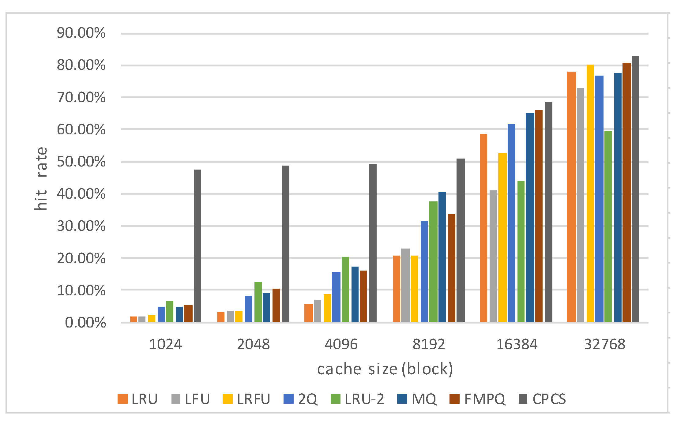
Besides the experiments on the parameter settings of the caching strategy, we also compared the hit rates of the cache under different algorithms. The experiment results are shown in Figure 14.
Figure 14 shows that when the cache sizes were 1024, 2048, 4096, 8192, 16,384 and 32,768, the hit rates of the cache under the CPCS were always higher than those under other cache strategies. The reason is that the data blocks in the cache under the CPCS are more effective. By exploring the relevance among data blocks, the blocks that are prefetched meet users’ needs in a short time. Moreover, the width of each batch in the TCFP-stream is set on the basis of the true situation in TC, and thus it is more suitable for the characteristics than other strategies.
However, from the growth-rate perspective, when the cache size was growing, the cache hits of other algorithms grew faster than those of the CPCS. The reason is that other algorithms, such as LRU, LFU, LFRU, 2Q, and LRU-2, place data blocks in the cache on the basis of the last recent access time or access frequency along with the system operation, which results in that these algorithms are weak on timeliness. These factors are also not absolute guarantees of data validity. Thus the effective data blocks may be squeezed out of the cache queue in a relatively short time as a new data stream becomes available, when the cache size is not large enough to store enough data. The effective data can also be retained in the cache for a longer time, and the hit rate of the cache will also be improved, when there is more space in the cache to retain more data. As for the CPCS algorithm, because the prefetched data blocks are strongly related to the data block accessed currently, more effective data blocks are prefetched in time, and the hit rate can reach a high degree, even if the cache size is not very large. Of course, if the cache size becomes larger, the cache will store more effective data. The hit rate of the cache becomes higher. Ultimately, the influence on hit rates made by the CPCS is based on the prefetched data blocks in time. This is why the impact of the cache size on hit rates in the CPCS algorithm is less than that in other algorithms.
5. Conclusions
This paper has proposed a CPCS in the TC server, according to the storage model and access characteristics of TC. In the CPCS, we improve the efficiency of the FP-stream’s mining frequent patterns and apply it to the data stream accessed in TC. The results of experiments show that different parameter settings contribute to different hit rates of the cache, and parameters are supposed to be adjusted to achieve optimal cache performance in polytropic environments and situation. Compared with LRU, LFU, LRFU, 2Q, LRU-2, MQ and FMPQ, CPCS is more specifically suitable to TC, particularly when the cache size is small. When facing a large number of resource service requests from the users, the improvements in cache performance can effectively reduce the I/O overhead of the server and then improve the efficiency of user access to server resources, ultimately enhancing the user experience. However, the parameters are configured according to the true situation in TC, so that a flexible and diverse cache scheduling strategy that can accommodate different runtime context environments is required. In the follow-on work, we will analyze the association between the accessed blocks and the users and further design a cache framework that can be coordinated between the client and the server.
Acknowledgments
This work was supported by the International Science & Technology Cooperation Program of China under Grant No. 2013DFB10070 and the China Hunan Provincial Science & Technology Program under Grant No. 2012GK4106.
Author Contributions
The study was carried out in collaboration between all authors. Jinfang Sheng and Bin Wang designed the research topic and checked the experimental results. Lin Chen and Weimin Li conducted the experiment, wrote the paper and examined the experimental data. All authors agreed to the submission of the manuscript.
Conflicts of Interest
The authors declare no conflict of interest.
References
- Wang, X.; Chen, M.; Taleb, T.; Ksentini, A.; Leung, V. Cache in the air: Exploiting content caching and delivery techniques for 5G systems. IEEE Commun. Mag. 2014, 52, 131–139. [Google Scholar] [CrossRef]
- Markakis, E.; Negru, D.; Bruneau-Queyreix, J.; Pallis, E.; Mastorakis, G.; Mavromoustakis, C. P2P Home-Box Overlay for Efficient Content Distribution. In Emerging Innovations in Wireless Networks and Broadband Technologies; IGI Global: Hershey, PA, USA, 2016; pp. 199–220. [Google Scholar]
- Shi, W.; Cao, J.; Zhang, Q.; Li, Y.; Xu, L. Edge Computing: Vision and Challenges. IEEE Internet Things J. 2016, 3, 637–646. [Google Scholar] [CrossRef]
- Zhang, Y.; Zhou, Y. Transparent Computing: A New Paradigm for Pervasive Computing; Springer: Berlin, Germany, 2006. [Google Scholar]
- Zhang, Y.; Guo, K.; Ren, J.; Zhou, Y.; Wang, J.; Chen, J. Transparent Computing: A Promising Network Computing Paradigm. Comput. Sci. Eng. 2017, 19, 7–20. [Google Scholar] [CrossRef]
- Gao, Y.; Zhang, Y.; Zhou, Y. Performance Analysis of Virtual Disk System for Transparent Computing. In Proceedings of the 9th International Conference on Ubiquitous Intelligence and Computing and 9th International Conference on Autonomic and Trusted Computing, Fukuoka, Japan, 4–7 September 2012; pp. 470–477. [Google Scholar]
- Gao, Y.; Zhang, Y.; Zhou, Y. A Cache Management Strategy for Transparent Computing Storage System; Springer: Berlin, Germany, 2006; pp. 651–658. [Google Scholar]
- Tang, Y.; Guo, K.; Tian, B. A block-level caching optimization method for mobile transparent computing. Peer Peer Netw. Appl. 2017, 1–12. [Google Scholar] [CrossRef]
- Guo, K.; Tang, Y.; Ma, J.; Zhang, Y. Optimized dependent file fetch middleware in transparent computing platform. Future Gener. Comput. Syst. 2015, 74, 199–207. [Google Scholar] [CrossRef]
- Liu, J.; Zhou, Y.; Zhang, D. TranSim: A Simulation Framework for Cache-Enabled Transparent Computing Systems. IEEE Trans. Comput. 2016, 65, 3171–3183. [Google Scholar] [CrossRef]
- Lin, K.W.; Chung, S.; Lin, C. A fast and distributed algorithm for mining frequent patterns in congested networks. Computing 2016, 98, 235–256. [Google Scholar] [CrossRef]
- Agrawal, R.; Srikant, R. Fast Algorithms for Mining Association Rules in Large Databases. In Proceedings of the 20th International Conference on Very Large Data Bases, Santiago de Chile, Chile, 12–15 September 1994; pp. 487–499. [Google Scholar]
- Han, J.; Pei, J.; Yin, Y. Mining Frequent Patterns without Candidate Generation. In Proceedings of the 2000 ACM SIGMOD International Conference on Management of Data, Dallas, TX, USA, 16–18 May 2000; pp. 1–12. [Google Scholar]
- Leung, C.K.; Khan, Q.I.; Li, Z.; Hoque, T. CanTree: a canonical-order tree for incremental frequent-pattern mining. Knowl. Inf. Syst. 2007, 11, 287–311. [Google Scholar] [CrossRef]
- Koh, Y.S.; Pears, R.; Dobbie, G. Extrapolation Prefix Tree for Data Stream Mining Using a Landmark Model; Springer: Berlin, Germany, 2012; pp. 340–351. [Google Scholar]
- Chen, X.j.; Ke, J.; Zhang, Q.q.; Song, X.p.; Jiang, X.m. Weighted FP-Tree Mining Algorithms for Conversion Time Data Flow. Int. J. Database Theor. Appl. 2016, 9, 169–184. [Google Scholar] [CrossRef]
- Ölmezoğulları, E.; Arı, İ.; Çelebi, Ö.F.; Ergüt, S. Data stream mining to address big data problems. In Proceedings of the Signal Processing and Communications Applications Conference (SIU), Haspolat, Turkey, 24–26 April 2013; pp. 1–4. [Google Scholar]
- Giannella, C.; Han, J.; Pei, J.; Yan, X.; Yu, P.S. Mining frequent patterns in data streams at multiple time granularities. Next Gener. Data Min. 2003, 212, 191–212. [Google Scholar]
- Zhang, Y. Transparence computing: Concept, architecture and example. Acta Electron. Sin. 2004, 32, 169–174. [Google Scholar]
- Zhang, Y.; Zhou, Y. 4VP: A Novel Meta OS Approach for Streaming Programs in Ubiquitous Computing. In Proceedings of the 21st International Conference on Advanced Information Networking and Applications (AINA 2007), Niagara Falls, ON, Canada, 21–23 May 2007; pp. 394–403. [Google Scholar]
- Zhang, Y.; Zhou, Y. Separating computation and storage with storage virtualization. Comput. Commun. 2011, 34, 1539–1548. [Google Scholar] [CrossRef]
- Chadha, V.; Figueiredo, R.J.O. ROW-FS: A User-Level Virtualized Redirect-on-Write Distributed File System for Wide Area Applications; Springer: Berlin, Germany, 2007; pp. 21–34. [Google Scholar]
- Ayres, J.; Flannick, J.; Gehrke, J.; Yiu, T. Sequential PAttern mining using a bitmap representation. In Proceedings of the Eighth ACM SIGKDD International Conference on Knowledge Discovery and Data Mining, Edmonton, AB, Canada, 23–26 July 2002; pp. 429–435. [Google Scholar]
- Chen, Y.; Dong, G.; Han, J.; Wah, B.W.; Wang, J. Multi-Dimensional Regression Analysis of Time-Series Data Streams. In Proceedings of the 28th International Conference on Very Large Data Bases, Hong Kong, China, 20–23 August 2002; pp. 323–334. [Google Scholar]
Figure 1.
Cumulative access frequency of data blocks.

Figure 2.
A pattern-tree model.

Figure 3.
The frequent pattern tree (FP-tree) structure constructed with the data in Table 1.
Figure 3.
The frequent pattern tree (FP-tree) structure constructed with the data in Table 1.

Figure 4.
The process of mining frequent patterns based on I6.

Figure 5.
Time period mapping in Figure 2.
Figure 5.
Time period mapping in Figure 2.

Figure 6.
Calculation for the top three recursions.
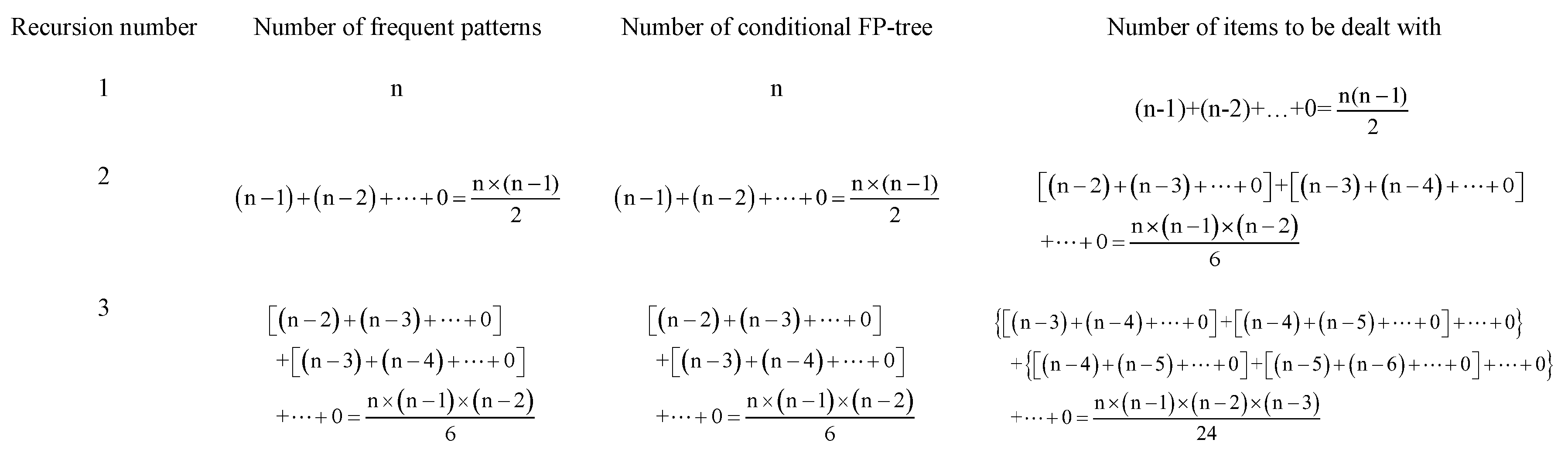
Figure 7.
The process of mining frequent patterns about I6 with changed method of mining frequent patterns by pattern fragment growth (FP-growth).
Figure 7.
The process of mining frequent patterns about I6 with changed method of mining frequent patterns by pattern fragment growth (FP-growth).
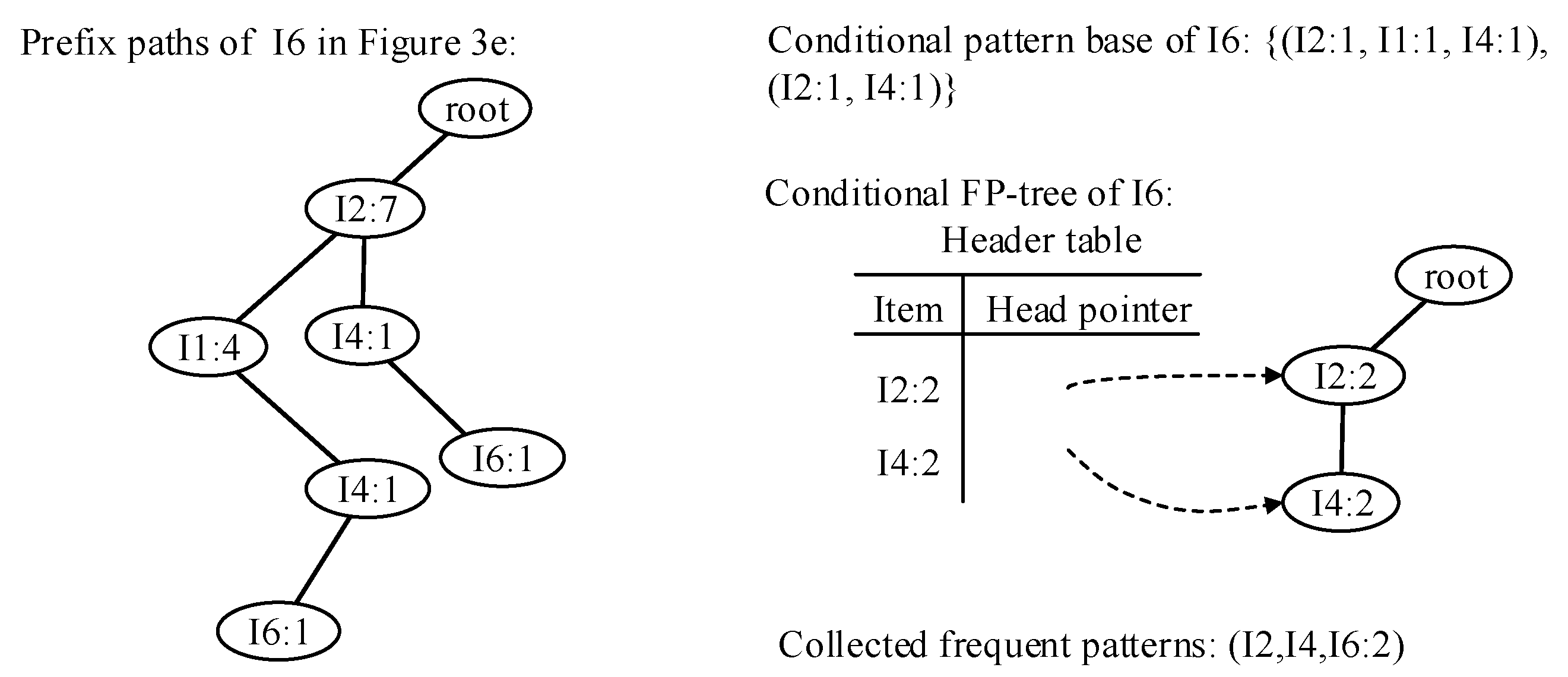
Figure 8.
The pattern-tree constructed with the data in Table 2.
Figure 8.
The pattern-tree constructed with the data in Table 2.

Figure 9.
Transparent computing (TC) pattern-tree updated with the data in Table 3.
Figure 9.
Transparent computing (TC) pattern-tree updated with the data in Table 3.

Figure 10.
Distribution of accessing intervals.
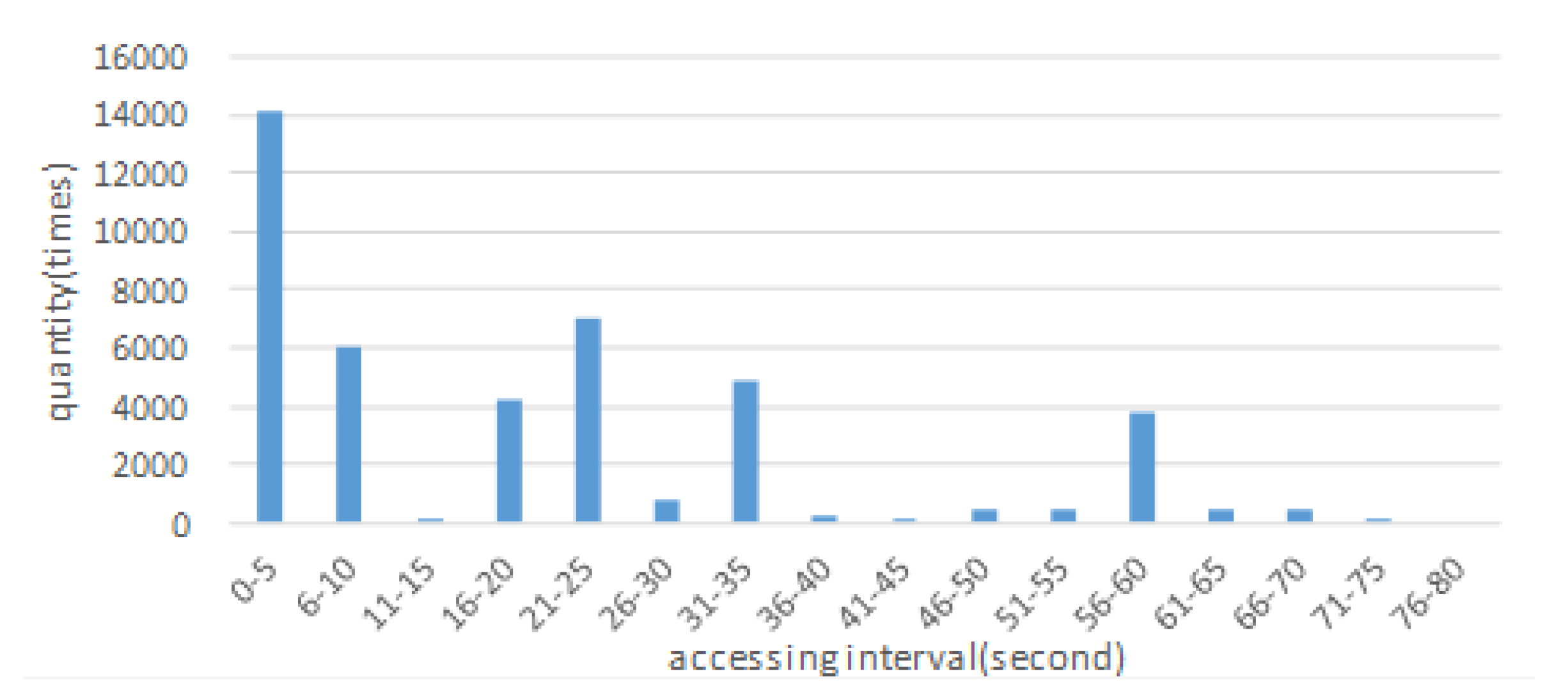
Figure 11.
A two-level cache model.
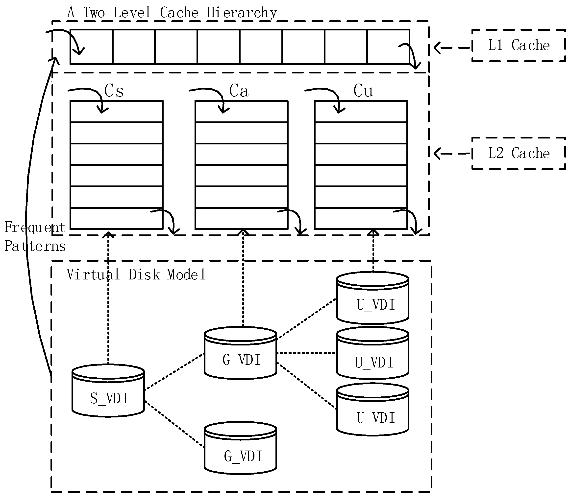
Figure 12.
Effects on hit rate of cache under different combinations of parameters.
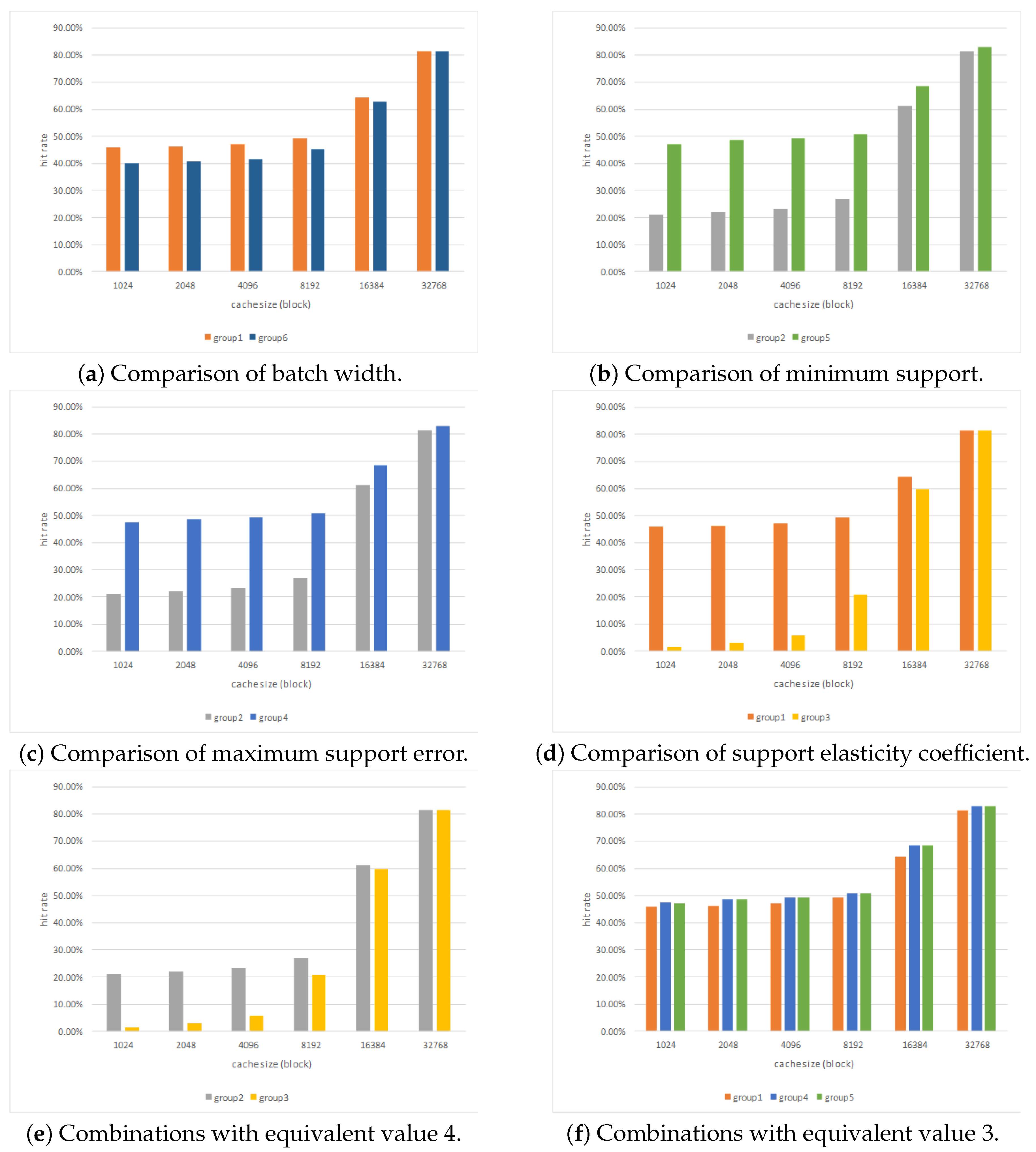
Figure 13.
Comparison of the efficiency of the frequent pattern tree-based model for mining frequent patterns from data streams (FP-stream) and the changed FP-stream for transparent computing (TCFP-stream).
Figure 13.
Comparison of the efficiency of the frequent pattern tree-based model for mining frequent patterns from data streams (FP-stream) and the changed FP-stream for transparent computing (TCFP-stream).
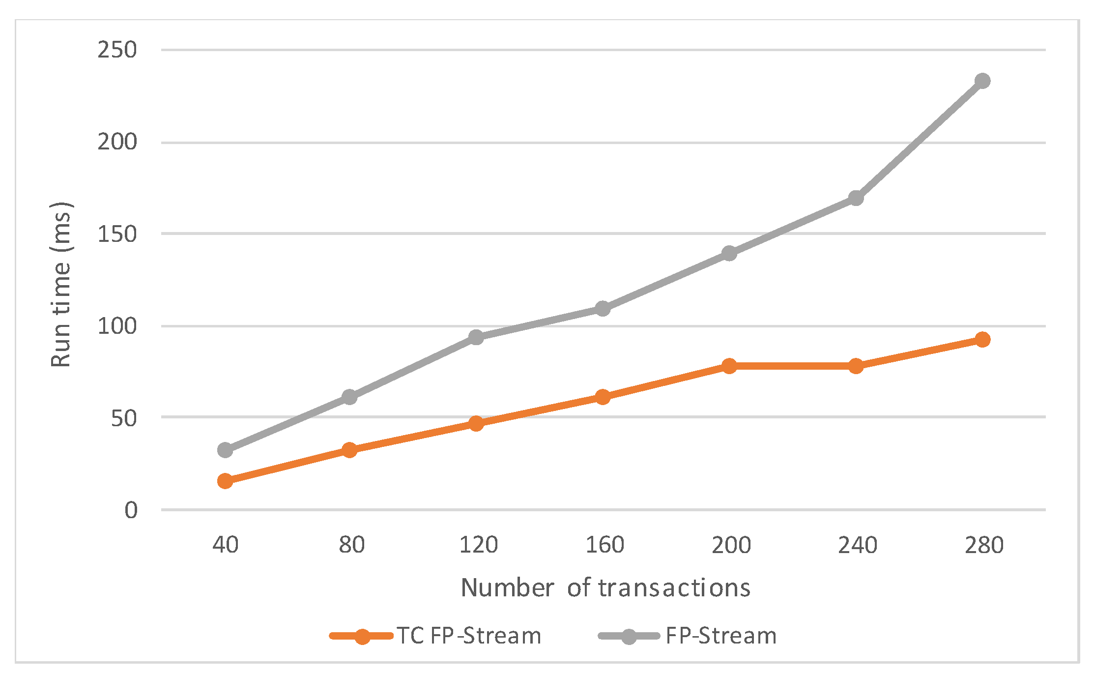
Figure 14.
Comparison of hit rate under different cache strategies.

Table 1.
Transaction database.
| Transaction Number | Items |
|---|---|
| 1 | I1,I2,I5 |
| 2 | I2,I4,I6 |
| 3 | I2,I3 |
| 4 | I1,I2,I4,I6 |
| 5 | I1,I3 |
| 6 | I2,I3 |
| 7 | I1,I3 |
| 8 | I1,I2,I3,I5 |
| 9 | I1,I2,I3 |
Table 2.
Frequent pattern table based on Figure 3.
Table 2.
Frequent pattern table based on Figure 3.
| Frequent Patterns | Support Count |
|---|---|
| 2 | |
| 2 | |
| 2 | |
| 2 | |
| 2 | |
| 2 | |
| 2 | |
| 2 | |
| 2 | |
| 2 | |
| 6 | |
| 4 | |
| 2 | |
| 4 | |
| 6 | |
| 4 | |
| 7 |
Table 3.
Frequent patterns based on Algorithm 1.
| Frequent Patterns | Support Count |
|---|---|
| 2 | |
| 2 | |
| 2 | |
| 4 | |
| 4 | |
| 2 | |
| 4 |
Table 4.
Several groups of parameter combinations.
| Group | Batch Width (s) | Minimum Support | Maximum Support Error | Support Elasticity Coefficient |
|---|---|---|---|---|
| Group 1 | 30 | 0.19 | 0.02 | 0.6 |
| Group 2 | 40 | 0.19 | 0.02 | 0.6 |
| Group 3 | 30 | 0.19 | 0.02 | 0.8 |
| Group 4 | 40 | 0.19 | 0.05 | 0.6 |
| Group 5 | 40 | 0.17 | 0.02 | 0.6 |
| Group 6 | 20 | 0.19 | 0.02 | 0.6 |
© 2018 by the authors. Licensee MDPI, Basel, Switzerland. This article is an open access article distributed under the terms and conditions of the Creative Commons Attribution (CC BY) license (http://creativecommons.org/licenses/by/4.0/).
Share and Cite
MDPI and ACS Style
Wang, B.; Chen, L.; Li, W.; Sheng, J. A Caching Strategy for Transparent Computing Server Side Based on Data Block Relevance. Information 2018, 9, 42. https://doi.org/10.3390/info9020042
AMA Style
Wang B, Chen L, Li W, Sheng J. A Caching Strategy for Transparent Computing Server Side Based on Data Block Relevance. Information. 2018; 9(2):42. https://doi.org/10.3390/info9020042
Chicago/Turabian StyleWang, Bin, Lin Chen, Weimin Li, and Jinfang Sheng. 2018. "A Caching Strategy for Transparent Computing Server Side Based on Data Block Relevance" Information 9, no. 2: 42. https://doi.org/10.3390/info9020042
Note that from the first issue of 2016, this journal uses article numbers instead of page numbers. See further details here.